Moving Manifolds in Electromagnetic Fields

1. Introduction

Fluid dynamics is one of the most well understood subjects in classical physics [1] and yet continues to be an actively developing field of research even today. Fluid dynamics can be treated as a motion of an inviscid fluid, as an indivisible medium of particles or as a collective motion of many body system particles. In the first case, when the fluid is inviscid and indivisible, the two conditions allow formulation of the Euler equation for dynamic fluid and the equation of continuity, where the Euler equation is a direct consequence of Newton's second law [1]. The second case is the most complicated and is difficult to treat. There are two possibilities for dealing with the second case: treat each separate particle as an individual one and propose that each particle satisfies Newton's laws of motion¹, or treat each particle as a vertex of a geometric figure and search for equations of motion for such geometries. If smoothed, the geometries, for a sufficient number of particles, can be modeled as continuously differentiable two manifolds embedded in Euclidean space (classical limit), or continuously differentiable three manifolds embedded in Minkowskian space-time (relativistic limit). Discussion of fluid dynamics in Minkowskian space-time corresponds to the fully relativistic formulation of the problem, while fluid dynamics in Euclidean space corresponds to the non-relativistic limit and is a specific case.

An example of fluid dynamics modeling as moving surfaces embedded in Euclidian space is moving two dimensional surfaces of fluid films such as soap films. Another, biologically relevant example is dynamic fluid membranes, vesicles, and micelles where a large body of notable theoretical results has already been produced [2, 3].

Soap films can be formed by dipping a closed contour wire or by dipping two rings into the soapy solution. Stationary fluid films or films in mechanical equilibrium with the environment form a surface with minimal surface area. Usually surfaces such as soap films are modeled as two dimensional manifolds. Fluid films not in mechanical equilibrium may have large displacements and can undergo big deformations [4–9]. The order of magnitude of thickness variations may vary from the nanometer to millimeter scale.

The equations of motion for free liquid films were initially proposed in Grinfeld [10] based on the least action principle of the Lagrangian:

$\begin{array}{rc}L=\frac{1}{2}{\displaystyle {\int }_S}\rho (C^2+V^2)dS-\sigma {\displaystyle {\int }_S}dS& (1)\end{array}$

where ρ is the two dimensional mass density of the fluid film, C is interface velocity, V is tangential velocity, σ is surface tension, S stands for the surface and free means that interactions with the ambient environment are ignored. Numerical solutions of the dynamic nonlinear equations for free thin fluid films display a number of new features consistent with experiments [8].

As indicated above, fluid dynamics can be described by motion of fluid surfaces, where the motion can happen in Euclidean ambient space, corresponding to the non-relativistic case or in Minkowski ambient space, corresponding to the fully relativistic case. Minkowskian space-time is more general and we will carry out derivations in Minkowski space that can be trivially simplified for non-relativistic cases. Instead of motion of free fluid films, we discuss motion of charged or partially charged material bodies with the boundary of charged or partially charged surfaces² in aqueous solution making hydrophobic-hydrophilic interactions. Hydrophobic-hydrophilic interactions are represented as electromagnetic interactions for reasons explained below. Representation of surfaces requires physical modeling and is illustrated in the physical models subsection for biomacromolecular surfaces. To be applicable to biological problems, we take the environment to be aqueous solution, though the medium does not directly enter into the general equations for free moving surfaces, so the equations can be applied to any moving surfaces in an electromagnetic field. We propose in this paper the modeling of fluid dynamics as moving surfaces in an electromagnetic field and consequently show that this concept non-trivially generalizes classical fluid dynamics. We pursue fully relativistic calculations because for biological macromolecules, femtosecond observations revealed that surface deformations, induced by dynamics of hydration at the surface or by charge transfer for proteins or DNA, usually happens on the angstrom to nanometer scale and may occur as fast as from femtosecond to picosecond [11, 12]. This sets upper limit for the interface velocity as high as C ~ nm/fs = 10⁶m/s and should be incorporated in a fully relativistic framework³.

The theoretical concept of hydrophobicity is already developed [13, 14] and is used to simulate shape dependence on hydrophobic interactions [15–18]. Although, the basic principles of the hydrophobic effect are qualitatively well understood, only recently have theoretical developments begun to explain quantitatively many features of the phenomenon [19].

Hydrophobic and hydrophilic interactions can be described as dispersive interactions between permanent or induced dipoles and ionic interactions throughout the molecules [19, 20]. Unification of all these interactions in one is the electromagnetic interaction's dependence on the interacting body's geometries [21–24]. To lay a foundation for the description of such geometric dependence, we give exact nonlinear equations governing geometric motion of the surface in an electromagnetic field set up by dipole moments of water molecules and partial charges of various molecules.

In this paper we discuss motion of compact and closed manifolds induced by electromagnetic field, where the field is generated by a continuously distributed charge in the material body. The boundary of the body is a semi-permeable surface (manifold) with a charge (or partial charge) and the charge can flow through the surface. Since, the charge in general is heterogeneously distributed in the body, the charge flow induces a time variable electromagnetic field on the surface of the body, forcing the motion of the manifold. Consequently, the problem is to find an equation of motion of moving manifolds in the electromagnetic field. The problem may be connected to many physics sub-fields, such as fluid dynamics, membrane dynamics or molecular surface dynamics. For instance the surface of macromolecules in aqueous solutions is permeable to some ions and water molecules and the charge on the surface is heterogeneously distributed. Flow of some ions and water molecules through the surface and the uneven distribution of charge in the macromolecules induce the surface dynamics. The same processes occur in biological membranes, vesicles, micelles, etc. Here we deduce general partial differential equations for moving manifolds in an electromagnetic field and demonstrate that the equations, in different conditions, simplify to the Euler equation for fluid dynamics, the Poisson-Boltzmann equation for describing the electric potential distribution on surface and the Maxwell equations for electrodynamics.

The formalism presented in this paper can be easily extended to hypersurfaces of any dimension. The limitation three surfaces embedded in four space-time, which is necessary to describe electromagnetism [25], is a consequence of specificity of the processes that take place on macromolecular surfaces. The time frame for dynamics of water molecules on the surface can be femtosecond range. Therefore, the surface can be charged with variable mass and charge densities and is continuously deformable. Mathematically the problem formulates as: find equations of motion in electromagnetic field for a closed, continuously differentiated and smooth two dimensional manifold in Euclidean space (non-relativistic case) or three manifolds in Minkowski spacetime (relativistic case). Dynamics of the surfaces under the influence of potential energy arises from four-potential time four-current and contraction of the electromagnetic tensor. Kinetic energy of the manifolds is calculated according to the calculus of moving surfaces [26]. Potential energy set by the object is modeled by the electromagnetic tensor the same way as for Maxwells equations. Definition of the Lagrangian [22] by subtracting potential energy from the kinetic energy and the minimum action principal yields nonlinear equations for moving surfaces in electromagnetic field.

2. Theoretical Preliminaries

2.1. Embedded Manifolds in Ambient Minkowski Space

Since Minkowskian space-time does not follow Riemannian geometry, we need a small adjustment of definitions. For Minkowski space-time, which fits to pseudo-Riemannian geometry, we need definitions of arbitrary base pairs of ambient space, even though the definitions look exactly the same as for Riemannian geometry embedded in Euclidean ambient space [26–28]. The summarized relationships about Riemannian geometry embedded in Euclidean space are given in tensor calculus text books [26, 27].

Combination of three ordinary dimensions with the single time dimension forms a four-dimensional manifold and represents Minkowski space-time. In this framework Minkowski four-dimensional space-time is the mathematical model of physical space in which Einsteins general theory is formulated. Minkowski space is independent of the inertial frame of reference and is a consequence of the postulates of special relativity [27, 29].

Euclidean space is the flat analog of Riemannian geometry while Minkowski space is considered as the flat analog of curved space-time, which is known in mathematics as pseudo-Riemannian geometry. Considerations of four-dimensional space-time make embedded moving manifolds three dimensional, where parametric time t, describing the motion of manifolds, may not have anything to do with proper time τ used in general relativity.

To briefly describe Minkowskian space-time, let us refer to arbitrary coordinates X^α, α = 0, …, 3, where the position vector R is expressed in coordinates as R = R(X^α). Bold letters throughout the manuscript designate vectors. Latin letters in indexes indicate surface related tensors. Greek letters in indexes show tensors related to the ambient space. All equations are fully tensorial and follow the Einstein summation convention.

Suppose that Sⁱ (i = 0, 1, 2) are the surface coordinates of the moving manifold S (Figure 1). Coordinates Sⁱ, X^α are arbitrarily chosen so that sufficient differentiation is achieved in both space and parametric time. The surface equation in ambient coordinates can be written as X^α = X^α(t, Sⁱ) and the position vector can be expressed as

$\begin{array}{rc}R=R(X^{\alpha })=R(t,S^i)& (2)\end{array}$

FIGURE 1

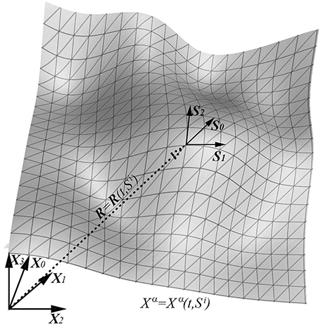
Figure 1. Two dimensional illustration of a curved three dimensional surface embedded in Minkowski space-time. X^α represents the analog of Cartesian coordinates of Minkowski space-time. S_i are base vectors defined in tangent space and X^α = X^α(t, Sⁱ) is the general equation of the surface.

Covariant bases for the ambient space are introduced as X_α = ∂_αR, where ${\partial }_{\alpha }=\partial /\partial X^{\alpha }$. The covariant metric tensor is the dot product of covariant bases

$\begin{array}{rc}{\eta }_{\alpha \beta }=X_{\alpha }·X_{\beta }& (3)\end{array}$

The contravariant metric tensor is defined as the matrix inverse of the covariant metric tensor, so that ${\eta }^{\alpha \nu }{\eta }_{\nu \beta }={\delta }_{\beta }^{\alpha }$, where ${\delta }_{\beta }^{\alpha }$ is the Kronecker delta. From definition (3) it follows that η₀₀ = X₀·X₀ and consequently if for Minkowskian space-time, the space like signature is set (−1, +1, +1, +1), then X₀ = (i, 0, 0, 0)⁴. Therefore, vector components are complex numbers in general. As far as the ambient space is set to be Minkowskian, the covariant bases are linearly independent, so that the square root of the negative metric tensor determinant is unit $\sqrt{-\left|{\eta }_{..}\right|}=1$. Furthermore, the Christoffel symbols given by

$\begin{array}{r}{\Gamma }_{\beta \gamma }^{\alpha }=X^{\alpha }·{\partial }_{\beta }{X}_{\gamma }\end{array}$

vanish and the equality between partial and curvilinear derivatives follows ∂_α = ∇_α. In Minkowski space-time (later space) the ∂_α partial derivative and ∇_α curvilinear derivative are the same. Everywhere in calculations we use ∂ letter for the ambient space derivative and keep in mind that when referring to Minkowski space the derivative has index in Greek letters and, in that case, it is the same as partial derivative. When indexes are mixed Greek and Latin letters the last statement, as is shown below, does not hold in general.

Now let's discuss tensors on the embedded surface with arbitrary coordinates Sⁱ, where i = 0, 1, 2. Latin indexes throughout the text are used exclusively for curved surfaces and curvilinear derivative ∇_i is no longer the same as the partial derivative ${\partial }_i=\partial /\partial S^i$. Similar to the bases of ambient space, covariant bases of an embedded manifold are defined as S_i = ∂_iR and the covariant surface metric tensor is the dot product of the covariant surface bases:

$\begin{array}{rc}{g}_{ij}=S_i·S_j& (4)\end{array}$

The definition (4) dictates that the surface is three dimensional pseudo Riemannian manifold, because ambient space is four dimensional Minkowskian space and the surface in four manifold is three manifold.

Analogically to space metric tensor g^ij the contravariant surface metric tensor is the matrix inverse of the covariant one g_ij. The matrix inverse nature of covariant-contravariant metrics gives possibility to raise and lower indexes of tensors defined on the manifold. The surface Christoffel symbols are given by

$\begin{array}{r}{\Gamma }_{jk}^i=S^i·{\partial }_j{S}_k\end{array}$

and along with Christoffel symbols of the ambient space provide all the necessary tools for covariant derivatives to be defined as tensors with mixed space/surface indexes:

$\begin{array}{c}{\nabla }_i{T}_{\beta k}^{\alpha j}={\partial }_i{T}_{\beta k}^{\alpha j}+{\eta }_i^{\gamma }{\Gamma }_{\gamma \nu }^{\alpha }{T}_{\beta k}^{\nu j}-{\eta }_i^{\gamma }{\Gamma }_{\gamma \beta }^{\mu }{T}_{\mu k}^{\alpha j}\\ +{\Gamma }_{im}^j{T}_{\beta k}^{\alpha m}-{\Gamma }_{ik}^m{T}_{\beta m}^{\alpha j}& (5)\end{array}$

where ${\eta }_i^{\gamma }$ is the shift tensor which reciprocally shifts space bases to surface bases, as well as space metric to surface metric. For instance, ${\mathbf{S}}_i={\eta }_i^{\alpha }{\mathbf{X}}_{\alpha }$ and

$\begin{array}{r}{g}_{ij}=S_i·S_j={\eta }_i^{\alpha }{X}_{\alpha }{\eta }_j^{\beta }{X}_{\beta }={\eta }_i^{\alpha }{\eta }_j^{\beta }{\eta }_{\alpha \beta }\end{array}$

The metrilinic property ∇_ig_mn = 0 of the surface metric tensor is a direct consequence of (4, 5) definitions, therefore S_m · ∇_iS_n = 0. The S_m and ∇_iS_n vectors are orthogonal, so that ∇_iS_n must be parallel to the N surface normal

$\begin{array}{rc}{\nabla }_i{S}_j=N{B}_{ij}& (6)\end{array}$

where B_ij is the tensorial coefficient of the (6) relationship and is generally referred to as the symmetric curvature tensor. The trace of the curvature tensor with upper and lower indexes is the mean curvature and its determinant is the Gaussian curvature. It is well-known that a surface with constant Gaussian curvature is a sphere, consequently a sphere can be expressed as:

$\begin{array}{rc}{B}_i^i=const& (7)\end{array}$

When the constant becomes null the surface becomes either a plane or a cylinder. Equation (7) is the expression of constant mean curvature (CMC) surfaces in general. Finding the curvature tensor defines the way of finding covariant derivatives of surface base vectors and so (6, 7) provide the way of finding surface base vectors which indirectly leads to the identification of the surface.

2.2. Differential Geometry for Embedded Moving Manifolds

After defining the metric tensor for ambient space η_μν (3) and the metric tensor for a moving surface g_ij (4), we now proceed with a brief review of surface velocity, t explicit (parametric) time derivative of surface tensors and time differentiation theorems for the surface/space integrals. The original definitions of time derivatives for moving surfaces were given in Hadamard [30] and recently extended in Grinfeld [26].

For the definition of surface velocity we need to define ambient coordinate velocity V^α first and to show that the coordinate velocity is the α component of the surface velocity. Indeed, by the velocity definition

$\begin{array}{rc}{V}^{\alpha }=\frac{\partial X^{\alpha }}{\partial t}& (8)\end{array}$

taking into account (2), R the position vector is tracking the material point coordinate Sⁱ. Therefore, by the partial time differentiation of (2) and definition of ambient base vectors, we find that V the surface velocity is

$\begin{array}{rc}V=\frac{\partial R(t,S^i)}{\partial t}=\frac{\partial R}{\partial X^{\alpha }}\frac{\partial X^{\alpha }(t,S^i)}{\partial t}=V^{\alpha }{X}_{\alpha }& (9)\end{array}$

Consequently V^α is the ambient component of the surface velocity. According to (9), the normal component of the surface velocity is the dot product with the surface normal

$\begin{array}{rc}C=V·N=V_{\alpha }{X}^{\alpha }{N}^{\beta }{X}_{\beta }=V_{\alpha }{N}^{\beta }{\eta }_{\beta }^{\alpha }=V_{\alpha }{N}^{\alpha }& (10)\end{array}$

The normal component C of the surface velocity is generally referred to as an interface velocity and is invariant in contrast with the coordinate velocity V^α. Its sign depends on a choice of the normal. The projection of the surface velocity on the tangent space (Figure 2) [28] is tangential velocity and can be expressed as

$\begin{array}{rc}{V}^i=V^{\alpha }{\eta }_{\alpha }^i& (11)\end{array}$

FIGURE 2

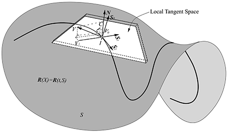
Figure 2. 2D Graphical illustration of the arbitrary chosen three manifold and it's local tangent space. S₀, S₁, S₂, and N are local tangent space base vectors and the normal, respectively. V is arbitrary chosen surface velocity and C, V_i, i = (0, 1, 2) display the projection of the velocity to the N, S_i directions.

Graphical illustrations of coordinate velocity V^α, interface velocity C and tangential velocity Vⁱ are given in Figure 2. The surface velocity V can be expressed as

$\begin{array}{rc}V=CN+V^i{S}_i& (12)\end{array}$

There is a clear geometric interpretation of the interface velocity [26, 28]. Let the surface at two nearby moments of time t and t + Δt be S_t, S_{t + Δt}. Suppose that A is a point on the S_t surface and the corresponding point B, belonging to S_{t + Δt}, has the same surface coordinate as A (Figure 3), then AB ≈ VΔt. Let P be the point where the unit normal N ∈ S_t intersects the surface S_t+Δt. Then for small enough Δt, the angle ∠APB ≈ π/2 and AP ≈ V · NΔt. Therefore, C can be defined as

$\begin{array}{r}C={\displaystyle \underset{\Delta t\to 0}{lim}}\frac{AP}{\Delta t}\end{array}$

and can be interpreted as the instantaneous velocity of the surface in the normal direction. It is worth mentioning that the sign of the interface velocity depends on the choice of the normal. Although, C is a scalar, it is called interface velocity because the normal direction is implied.

FIGURE 3

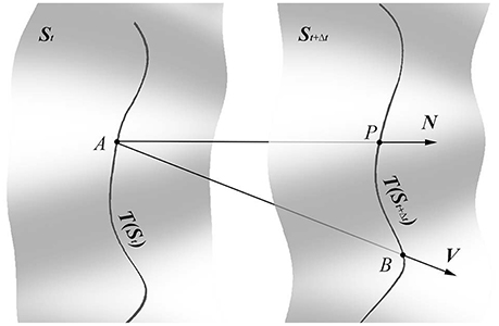
Figure 3. Geometric interpretation of the invariant time derivative $\stackrel{·}{\nabla }$ applied to invariant tensor field T. A is an arbitrarily chosen point on the S_t surface so that it lies on the T(S_t) curve. B is the corresponding point on the S_t+Δt surface. P is the point where the S_t surface normal, applied on the point A, intersects the surface S_t+Δt. For infinitely small Δt AB ≈ VΔt and AP ≈ V · NΔt. According to the geometric construction the tensor field T at the point B can be estimated as T(B) ≈ T(A) + Δt∂T/∂t, while T(B) can be estimated by the covariant surface derivative $T(B)\approx T(P)+\Delta t{V}^i{\nabla }_{i}T$, where ∇_iT shows rate of change in T along the directed distance BP ≈ ΔtVⁱ on the surface S_t+Δt.

2.3. Time Derivative

In this section we briefly explain the concept behind the invariant time derivative for scalar and tensor fields defined on moving manifolds, even though these concepts are already given [26]. Suppose that invariant tensor field T is defined on the manifold at all time. To define the time invariant derivative of the tensor field it is necessary to capture the rate of change of T in the normal direction. The physical explanation of why the deformations along the normal direction are so important is given below when discussing integrals. This is similar to how C measures the rate of deformation in the normal direction. For a given point A ∈ S_t, find the point B ∈ S_t+Δt and P the intersection of S_t+Δt and the straight line orthogonal to S_t (Figure 3). Then the geometrically intuitive definition dictates that

$\begin{array}{rc}\stackrel{·}{\nabla }T={\displaystyle \underset{\Delta t\to 0}{lim}}\frac{T(P)-T(A)}{\Delta t}& (13)\end{array}$

Because (13) is entirely geometric, it must be free from choice of a reference frame. Therefore, it is invariant. On the other hand, from the geometric construction it follows that

$\begin{array}{rc}T(B)\approx T(A)+\Delta t\frac{\partial T}{\partial t}& (14)\end{array}$

T(B) is related to T(P) because B,P are nearby points and are situated on the S_t+Δt surface B, P ∈ S_{t + Δt}. Then

$\begin{array}{rc}T(B)\approx T(P)+\Delta t{V}^i{\nabla }_{i}T& (15)\end{array}$

since ∇_iT shows rate of change in the tensor field along the surface and ΔtVⁱ indicates the directed distance BP. After a few lines of algebra, taking into account Equations (14, 15) in (13), we find

$\begin{array}{rc}\stackrel{·}{\nabla }T=\frac{\partial T}{\partial t}-V^i{\nabla }_{i}T& (16)\end{array}$

Generalization of (16) to any arbitrary tensors with mixed space and surface indexes is given by the formula

$\begin{array}{l}\stackrel{·}{\nabla }{T}_{\beta j}^{\alpha i}=\frac{\partial T_{\beta j}^{\alpha i}}{\partial t}-V^k{\nabla }_k{T}_{\beta j}^{\alpha i}+V^{\gamma }{\Gamma }_{\gamma \mu }^{\alpha }{T}_{\beta j}^{\mu i}-V^{\gamma }{\Gamma }_{\gamma \beta }^{\mu }{T}_{\mu j}^{\alpha i}\\ +{\stackrel{·}{\Gamma }}_k^i{T}_{\beta j}^{\alpha k}-{\stackrel{·}{\Gamma }}_j^k{T}_{\beta k}^{\alpha i}& (17)\end{array}$

where Christoffel symbol ${\stackrel{·}{\Gamma }}_m^n$ for moving surfaces is ${\stackrel{·}{\Gamma }}_m^n={\nabla }_m{V}^n-C{B}_m^n$. The derivative commutes with contraction, satisfies sum, product and chain rules, is metrinilic with respect to the ambient metrics and does not commute with the surface derivative [26]. Also from (13) it is clear that the invariant time derivative applied to the time independent scalar vanishes.

2.4. Time Derivatives of Space/Surface Integrals

Time differentiation of surface and space integrals have a central role in evaluation of the principle of least action. Dependence of time variation of the potential energy on the geometry becomes rigorously clarified from these theorems. For any scalar field T = T(t, Sⁱ) defined on a Minkwoskian domain Ω with boundary S manifold evolving with the interface velocity C, the evolution of the space integral and surface integral for closed compact manifolds are given by the formulas

$\begin{array}{cc}\frac{d}{dt}{\displaystyle {\int }_{\Omega }Td\Omega }={\displaystyle {\int }_{\Omega }\frac{\partial T}{\partial t}d\Omega }+{\displaystyle {\int }_{S}CTdS}& (18)\end{array}$

$\begin{array}{cc}\frac{d}{dt}{\displaystyle {\int }_{S}TdS}={\displaystyle {\int }_S\dot{\nabla }TdS}-{\displaystyle {\int }_{S}CT{B}_i^{i}dS}& (19)\end{array}$

The first term in the integral represents the rate of change of the tensor field, while the second term shows changes in the geometry. It therefore properly takes into account the convective and advective terms due to volume motion. We are not going to reproduce proof of these theorems here⁵, but instead we give intuitive explanation of why only interface velocity has a role and tangential velocities do not appear in the integration. If the surface velocity has no interface velocity and has only tangential components, then the tangent velocity translates each point to it's neighboring ones and does not add new area and volume to the surface and space. Therefore, it provokes rotational movement of the material object and can be excluded from the integration. This statement becomes obvious for one dimensional motion. If the material point is moving along some trajectory, then the velocity is tangential to the curve. However, motion of the material point along the curve can be understood as the motion of the curve embedded in the plane. If the curve has no interface velocity, then it only slides in the ambient plane without changing the local length⁶.

2.5. Several Useful Theorems

In this section we provide several theorems, that will be directly used to deduce equations of motions. The first such theorem is the general Gauss theorem about integration, which gives the rule for the reciprocal transfer of space integral to surface integral. For a domain Ω in Minkowski space with the boundary S, for any sufficiently smooth tensor field T^α, the generalized Gauss theorem reads

$\begin{array}{cc}{\displaystyle {\int }_{\Omega }}{\nabla }_{\alpha }{T}^{\alpha }d\Omega ={\displaystyle {\int }_S}{N}_{\alpha }{T}^{\alpha }dS& (20)\end{array}$

The proof is simple if one uses the Voss-Weyl formula to deduce the theorem. For any sufficiently smooth tensor field in Minkowski space, the Voss-Weyl formula [26] reads

$\begin{array}{rc}{\nabla }_{\mu }{T}^{\mu }=\frac{1}{\sqrt{-\left|{\eta }_{..}\right|}}{\partial }_{\mu }(\sqrt{-\left|{\eta }_{..}\right|}{T}^{\mu })& (21)\end{array}$

Using (21) in the right part of (20) and the designation η = −|η_..|, we have

$\begin{array}{l}{\displaystyle {\int }_{\Omega }{\nabla }_{\alpha }}{T}^{\alpha }d\Omega ={\displaystyle {\int }_{\Omega }\frac{1}{\sqrt{\eta }}}{\partial }_{\mu }(\sqrt{\eta }{T}^{\mu })d\Omega \\ =\int \text{}\int \text{}\int \text{}\int \frac{1}{\sqrt{\eta }}{\partial }_{\mu }(\sqrt{\eta }{T}^{\mu })\sqrt{\eta }d{X}^{\alpha }\\ =\int \text{}\int \text{}\int \text{}\int {\partial }_{\mu }(\sqrt{\eta }{T}^{\mu })d{X}^{\alpha }\end{array}$

where dX^α = dX⁰dX¹dX²dX³. This term is subject to the Gausss theorem in the arithmetic space. Since arithmetic space and Minkowski space, which is pseudo-Euclidean, can be related to Cartesian coordinates, Minkowski space can be identified as an arithmetic one and the Gauss theorem for the arithmetic space can be used. Thus, using unity of the Minkowski space metric tensor determinant one may prove that⁷

$\begin{array}{l}\int \text{}\int \text{}\int \text{}\int {\partial }_{\mu }(\sqrt{\eta }{T}^{\mu })d{X}^{\alpha }={\displaystyle \iiint N_{\alpha }}{T}^{\alpha }\sqrt{\eta }\sqrt{g}d{S}^i\\ ={\displaystyle {\int }_S{N}_{\alpha }}{T}^{\alpha }dS\end{array}$

where g = |g_..|. This proves that the generalized Gauss's theorem holds for pseudo-Riemannian manifolds embedded in Minkowski space.

The next step is to provide short proofs for Weingarten's and Thomas' formulas by using the relation between the surface derivative and the interface velocity.

Weingarten's formula expresses the surface covariant derivative of the surface normal in the product of the shift and mixed curvature tensors. Proof follows from the definition $N_{\alpha }{N}^{\alpha }=1$, from which we find $N_{\alpha }{\nabla }_i{N}^{\alpha }=0$. On the other hand

$\begin{array}{l}0=N·S_i=N^{\alpha }{X}_{\alpha }·{\eta }_i^{\beta }{X}_{\beta }=N^{\alpha }{\eta }_i^{\beta }{\eta }_{\alpha \beta }\\ =N^{\alpha }{\eta }_{\alpha i}& (22)\end{array}$

If we apply the covariant derivative to (22) and take into account that from (6) $B_{ji}=N^{\alpha }{\nabla }_j{\eta }_{i\alpha }$ then by the product rule we find

$\begin{array}{l}0={\nabla }_j{N}^{\alpha }{\eta }_{\alpha i}+N^{\alpha }{\nabla }_j{\eta }_{\alpha i}={\nabla }_j{N}^{\alpha }{\eta }_{\alpha i}+B_{ji}\\ {\nabla }_j{N}^{\alpha }{\eta }_{\alpha i}=-B_{ji}& (23)\end{array}$

Let's contract both sides of (23) with η^iβ and take into account the commonly used relationship in tensor calculus $N^{\alpha }{N}_{\beta }+{\eta }_i^{\alpha }{\eta }_{\beta }^i={\delta }_{\beta }^{\alpha }$, then we find

$\begin{array}{l}-{\eta }_k^{\beta }{B}_j^k=-{\eta }^{i\beta }{B}_j^k{g}_{ki}=-{\eta }^{i\beta }{B}_{ji}={\nabla }_j{N}^{\alpha }{\eta }_{\alpha i}{\eta }^{i\beta }\\ ={\nabla }_j{N}^{\alpha }{\eta }_{\alpha }^k{g}_{ik}{\eta }_m^{\beta }{g}^{mi}={\nabla }_j{N}^{\alpha }{\eta }_{\alpha }^k{\eta }_m^{\beta }{\delta }_k^m\\ ={\nabla }_j{N}^{\alpha }{\eta }_{\alpha }^k{\eta }_k^{\beta }={\nabla }_j{N}^{\alpha }({\delta }_{\alpha }^{\beta }-N^{\beta }{N}_{\alpha })\\ ={\nabla }_j{N}^{\beta }-N^{\beta }{N}_{\alpha }{\nabla }_j{N}^{\alpha }\\ {\nabla }_j{N}^{\beta }=-{\eta }_k^{\beta }{B}_j^k& (24)\end{array}$

Since the second term of the last equality vanishes, we get (24), also known as Weingarten's formula.

Now we turn to the Thomas formula which allows calculation of the invariant time derivative of the surface normal. Indeed, using the invariant time derivative formula for the surface base vector [26]

$\begin{array}{rc}\stackrel{·}{\nabla }{S}_i=N{\nabla }_{i}C& (25)\end{array}$

and dotting both sides of (25) with N, $N·\stackrel{·}{\nabla }{\mathbf{S}}_i=\mathit{N}·N{\nabla }_{i}C$ and using the product rule, taking into account that N · S_i = 0, we find ${\nabla }_{i}C=-\stackrel{·}{\nabla }\mathit{N}{\mathbf{S}}_i$, therefore

$\begin{array}{rc}\stackrel{·}{\nabla }N=-S^i{\nabla }_{i}C& (26)\end{array}$

Equation (26) is generally referred to as the Thomas formula.

3. Equations of Motion and Physical Models

3.1. Equations of Motion

Since we have all mathematical preliminaries in hand we can proceed with derivation of master equations of motion. To derive the equations we apply the calculus of moving surfaces to the motion of compact and closed manifolds in an electromagnetic field. In this step we only discuss free motion of the single closed surface, where “single” surface means boundary of the single material body and “free” means contact with environment is ignored⁸. The interaction with the environment can be incorporated into the equations later on⁹. The surface is treated as a continuum medium of material particles (points), where charge and mass distribution is heterogeneous. The boundary of the body is the surface with a surface mass density ρ and a surface charge density q. The surface can be semipermeable at some material points, meaning the charge can flow through the surface. Interaction between the material points is exclusively electromagnetic, as the mass of each material particle is set to be infinitely small compared to unit charges. The ambient space is set to be Minkowskian, the body is four dimensional and has the surface boundary of three dimensional manifold. Electromagnetic interaction between the material particles and the heterogeneous distribution of charges throughout the object induces motion of the surface and the potential energy of the interaction can be modeled as

$\begin{array}{cc}{U}={\displaystyle {\int }_{\Omega }(\frac{1}{4{\mu }_0}{F}_{\alpha \beta }{F}^{\alpha \beta }+A_{\alpha }{J}^{\alpha })}d\Omega & \left(27\right)\end{array}$

where the electromagnetic tensor F_αβ is the combination of the electric and magnetic fields in a covariant antisymmetric tensor [25, 29]. The electromagnetic covariant four-potential is a covariant four vector A_· = (−φ/c, a) composed of the φ electric potential and the a magnetic potential. Contravariant four current J^· = (cQ, j) is the contravariant four vector combining j electric current density and Q the charge density, c is the speed of light and μ₀ is the magnetic permeability of the vacuum. The Minkowski space metric tensor signature is set to be space-like (− + + +) throughout the paper. This formulation is fully relativistic though it can be easily simplified for non-relativistic cases. Raising and lowering the indexes is performed by the Minkowski metric η_αβ. The relation between the four potentials and the electromagnetic tensor is given by

$\begin{array}{cc}{F}_{\alpha \beta }={\partial }_{\alpha }{A}_{\beta }-{\partial }_{\beta }{A}_{\alpha }& \left(28\right)\end{array}$

As far as the boundary of the material body is a moving three manifold, the surface kinetic energy with variable surface mass density ρ and surface velocity V is

$\begin{array}{cc}{T}={\displaystyle {\int }_S\frac{\rho V^2}{2}}dS& \left(29\right)\end{array}$

Subtraction of the potential energy (27) from the kinetic energy (29) leads to the system Lagrangian

$\begin{array}{cc}{L}={\displaystyle {\int }_S\frac{\rho V^2}{2}}dS-{\displaystyle {\int }_{\Omega }(\frac{1}{4{\mu }_0}{F}_{\alpha \beta }{F}^{\alpha \beta }+A_{\alpha }{J}^{\alpha })}d\Omega & \left(30\right)\end{array}$

where S is the boundary of Ω. Hamilton's least action principle [31] for the given Lagrangian (30) reads

$\begin{array}{cc}\frac{\delta {L}}{\delta t}=\frac{\delta {T}}{\delta t}-\frac{\delta {U}}{\delta t}=0& \left(31\right)\end{array}$

For proper evaluation of the (31) Lagrangian we start from the simplest term first, the potential energy. Since (27) is the space integral by theorem (18) we have

$\begin{array}{cc}\begin{array}{l}\frac{\delta {U}}{\delta t}={\displaystyle {\int }_{\Omega }\frac{\partial }{\partial t}}(\frac{1}{4{\mu }_0}{F}_{\alpha \beta }{F}^{\alpha \beta }+A_{\alpha }{J}^{\alpha })d\Omega \\ +{\displaystyle {\int }_{S}C}(\frac{1}{4{\mu }_0}{F}_{\alpha \beta }{F}^{\alpha \beta }+A_{\alpha }{J}^{\alpha })dS\end{array}& \left(32\right)\end{array}$

According to (32) determination of variation of potential energy is calculated from the time differential of the space integrand. Following standard algebraic manipulations for classical electrodynamics, we find

$\begin{array}{cc}\begin{array}{l}{\displaystyle {\int }_{\Omega }\frac{\partial u}{\partial t}}d\Omega ={\displaystyle {\int }_{\Omega }(\frac{\partial u}{\partial A_{\alpha }}\frac{\partial A_{\alpha }}{\partial t}+\frac{\partial u}{\partial ({\partial }_{\beta }{A}_{\alpha })}\frac{\partial ({\partial }_{\beta }{A}_{\alpha })}{\partial t})}d\Omega \\ ={\displaystyle {\int }_{\Omega }(\frac{\partial u}{\partial A_{\alpha }}\frac{\partial A_{\alpha }}{\partial t}+{\partial }_{\beta }(}\frac{\partial u}{\partial ({\partial }_{\beta }{A}_{\alpha })}\frac{\partial A_{\alpha }}{\partial t})\\ -{\partial }_{\beta }\frac{\partial u}{\partial ({\partial }_{\beta }{A}_{\alpha })}\frac{\partial A_{\alpha }}{\partial t})d\Omega \\ ={\displaystyle {\int }_{\Omega }(\frac{\partial u}{\partial A_{\alpha }}\frac{\partial A_{\alpha }}{\partial t}-{\partial }_{\beta }\frac{\partial u}{\partial ({\partial }_{\beta }{A}_{\alpha })}\frac{\partial A_{\alpha }}{\partial t})}d\Omega \\ +\frac{\partial u}{\partial ({\partial }_{\beta }{A}_{\alpha })}\frac{\partial A_{\alpha }}{\partial t}{|}_{\frac{\partial A_{\alpha }}{\partial t}=0}\\ ={\displaystyle {\int }_{\Omega }(\frac{\partial u}{\partial A_{\alpha }}-{\partial }_{\beta }\frac{\partial u}{\partial ({\partial }_{\beta }{A}_{\alpha })})}\frac{\partial A_{\alpha }}{\partial t}d\Omega \end{array}& \left(33\right)\end{array}$

where $u=(1/4{\mu }_0)F_{\mu \nu }{F}^{\mu \nu }+A_{\mu }{J}^{\mu }$ and the fact that u is a function of A_α and ∂_βA_α and at the boundary condition ∂A_α/∂t = 0 the last term vanishes. It is easy to show that,

$\begin{array}{cc}\partial u/\partial A_{\alpha }=J^{\alpha }& \left(34\right)\end{array}$

To calculate the last integrand (33), we take into account the definition (28) and note that the covariant electromagnetic tensor can be obtained by lowering indexes in contravariant tensor $F^{\alpha \beta }={\eta }^{\gamma \alpha }{\eta }^{\kappa \beta }{F}_{\gamma \kappa }$. The electromagnetic tensor is antisymmetric F^αβ = −F^βα, so that

$\begin{array}{cc}\begin{array}{l}\frac{\partial u}{\partial ({\partial }_{\beta }{A}_{\alpha })}=\frac{1}{4{\mu }_0}\frac{\partial }{\partial ({\partial }_{\beta }{A}_{\alpha })}(F_{\mu \nu }{\eta }^{\gamma \mu }{\eta }^{\lambda \nu }{F}_{\gamma \lambda })\\ =\frac{1}{4{\mu }_0}{\eta }^{\gamma \mu }{\eta }^{\lambda \nu }\frac{\partial (F_{\mu \nu }{F}_{\gamma \lambda })}{\partial ({\partial }_{\beta }{A}_{\alpha })}\\ =\frac{1}{4{\mu }_0}{\eta }^{\gamma \mu }{\eta }^{\lambda \nu }(F_{\mu \nu }({\delta }_{\gamma }^{\beta }{\delta }_{\lambda }^{\alpha }-{\delta }_{\lambda }^{\beta }{\delta }_{\gamma }^{\alpha })\\ +F_{\gamma \lambda }({\delta }_{\mu }^{\beta }{\delta }_{\nu }^{\alpha }-{\delta }_{\nu }^{\beta }{\delta }_{\mu }^{\alpha }))\\ =\frac{1}{4{\mu }_0}(F^{\beta \alpha }-F^{\alpha \beta }+F^{\beta \alpha }-F^{\alpha \beta })=\frac{F^{\beta \alpha }}{{\mu }_0}\\ \end{array}& \left(35\right)\end{array}$

Taking into account (33–35) in (32) we find the variation of the potential energy

$\begin{array}{cc}\begin{array}{l}\frac{\delta {U}}{\delta t}={\displaystyle {\int }_{\Omega }(J^{\alpha }-\frac{1}{{\mu }_0}{\partial }_{\beta }{F}^{\beta \alpha })}\frac{\partial A_{\alpha }}{\partial t}d\Omega \\ +{\displaystyle {\int }_{S}C}(\frac{1}{4{\mu }_0}{F}_{\alpha \beta }{F}^{\alpha \beta }+A_{\alpha }{J}^{\alpha })dS\end{array}& \left(36\right)\end{array}$

Now we turn to the calculation of the kinetic energy variation. To deduce the variation for the kinetic energy let's define the generalization of conservation of mass law first. The variation of the surface mass density must be so that dm/dt = 0, where

$\begin{array}{cc}m={\displaystyle {\int }_S\rho }dS& \left(37\right)\end{array}$

is the surface mass with ρ surface mass density. Since we discuss compact closed manifolds the boundary conditions $v=n_i{V}^i=0$ dictate that a pass integral along any curve across the surface must vanish. This statement formally taking into consideration (37), can be rewritten as

$\begin{array}{cc}\begin{array}{l}0={\displaystyle {\int }_{\gamma }v}\rho d\gamma ={\displaystyle {\int }_{\gamma }{n}_i}{V}^i\rho d\gamma ={\displaystyle {\int }_S{\nabla }_i}(\rho V^i)dS\\ ={\displaystyle {\int }_S({\nabla }_i(}\rho V^i)-\rho C{B}_i^i+\rho C{B}_i^i)dS\\ ={\displaystyle {\int }_S({\nabla }_i(}\rho V^i)-\rho C{B}_i^i)dS+{\displaystyle {\int }_S\dot{\nabla }}\rho dS-\frac{d}{dt}{\displaystyle {\int }_S\rho }dS\\ ={\displaystyle {\int }_S({\nabla }_i(}\rho V^i)-\rho C{B}_i^i+\dot{\nabla }\rho )dS\end{array}& \left(38\right)\end{array}$

where n is a normal of the curve that lies in the tangent space, v is the velocity of the γ curve. Since the last integral from (38) mast be identical to zero for any integrand, one immediately finds the generalization of conservation of mass law

$\begin{array}{cc}\dot{\nabla }\rho +{\nabla }_i(\rho V^i)=\rho C{B}_i^i& \left(39\right)\end{array}$

Incidentally, an equation for the surface charge conservation can analogously be deduced and it has exactly the same form. The equation (39) was also reported in Grinfeld [10]. To calculate the variation of the kinetic energy we use (19, 29, 39) and after a few lines of algebra, we find

$\begin{array}{cc}\begin{array}{l}\frac{\delta {T}}{\delta t}={\displaystyle {\int }_S(\dot{\nabla }\frac{\rho V^2}{2}-C{B}_i^i\frac{\rho V^2}{2})}dS\\ ={\displaystyle {\int }_S(\dot{\nabla }\rho \frac{V^2}{2}+\rho \dot{\nabla }\frac{V^2}{2}-C{B}_i^i\frac{\rho V^2}{2})}dS\\ ={\displaystyle {\int }_S((}\rho C{B}_i^i-{\nabla }_i(\rho V^i))\frac{V^2}{2}+\rho \dot{\nabla }\frac{V^2}{2}-C{B}_i^i\frac{\rho V^2}{2})dS\\ ={\displaystyle {\int }_S(-{\nabla }_i(}\rho V^i\frac{V^2}{2})+\rho V^i{\nabla }_i\frac{V^2}{2}+\rho \dot{\nabla }\frac{V^2}{2})dS\\ ={\displaystyle {\int }_S\rho }V(V^i{\nabla }_{i}V+\dot{\nabla }V)dS\end{array}& \left(40\right)\end{array}$

Here we used the fact that at the end of variations the surface reaches the stationary point and therefore, by the Gauss theorem integral for ${\nabla }_i(\rho V^i{V}^2/2)$ converted to line integral, vanishes [as we used it already in (38)]. To deduce the final form of equations of motion we decompose the dot product in the integral (40) into normal and tangential components. After a few lines of algebraic manipulations, we find

$\begin{array}{cc}\begin{array}{l}\dot{\nabla }V+V^i{\nabla }_{i}V=\dot{\nabla }V+V^i{\nabla }_{i}V+C{V}^i{B}_i^j{S}_j-C{V}^i{B}_i^j{S}_j\\ =\dot{\nabla }V+V^i{\nabla }_{i}V+C{V}^i{B}_i^j{\eta }_j^{\alpha }{X}_{\alpha }-C{V}^i{B}_i^j{S}_j\end{array}& \left(41\right)\end{array}$

Using Weingartens formula (24), the metrilinic property of the Minkowski space base vectors ∇_iX_α = 0 and the definition of the surface normal $\mathbf{N}=N^{\alpha }{\mathbf{X}}_{\alpha }$, the last equation of (41) transforms

$\begin{array}{cc}\begin{array}{l}\dot{\nabla }V+V^i{\nabla }_{i}V-C{V}^i{X}_{\alpha }{\nabla }_i{N}^{\alpha }-C{V}^i{B}_i^j{S}_j\\ =\dot{\nabla }V+V^i{\nabla }_{i}V-C{V}^i{\nabla }_{i}N-C{V}^i{B}_i^j{S}_j\end{array}& \left(42\right)\end{array}$

Taking into account (12) and its covariant and invariant time derivatives in (42), we find

$\begin{array}{cc}\begin{array}{l}\dot{\nabla }V+V^i{\nabla }_i(CN)+V^i{\nabla }_i(V{S}_j)\\ -C{V}^i{\nabla }_{i}N-C{V}^i{B}_i^j{S}_j\\ \text{}=\dot{\nabla }V+V^{i}N{\nabla }_{i}C+V^i{\nabla }_i(V^j{S}_j)-C{V}^i{B}_i^j{S}_j\\ =\dot{\nabla }(CN)+\dot{\nabla }(V^j{S}_j)+V^{i}N{\nabla }_{i}C\\ +V^i{\nabla }_i(V^j{S}_j)-C{V}^i{B}_i^j{S}_j\end{array}& \left(43\right)\end{array}$

Continuing algebraic manipulations using the formula for the surface derivative of the interface velocity (25), Thomas formula (26), and the definition of the curvature tensor (6) in (43), yield

$\begin{array}{cc}\begin{array}{l}\dot{\nabla }(CN)+C{\nabla }^{j}C{S}_j+2V^{i}N{\nabla }_{i}C+V^i{V}^j{B}_{ij}N\\ +\dot{\nabla }(V^j{S}_j)-V^{i}N{\nabla }_{i}C+V^i{\nabla }_i(V^j{S}_j)-V^i{V}^j{B}_{ij}N\\ -C{\nabla }^{j}C{S}_j-C{V}^i{B}_i^j{S}_j\\ =\dot{\nabla }(CN)-C\dot{\nabla }N+2V^{i}N{\nabla }_{i}C+V^i{V}^j{B}_{ij}N\\ +\dot{\nabla }(V^j{S}_j)-V^j\dot{\nabla }{S}_j+V^i{\nabla }_i(V^j{S}_j)-V^i{V}^j{\nabla }_i{S}_j\\ -C{\nabla }^{j}C{S}_j-C{V}^i{B}_i^j{S}_j\\ =(\dot{\nabla }C+2V^i{\nabla }_{i}C+V^i{V}^j{B}_{ij})N\\ +(\dot{\nabla }{V}^j+V^i{\nabla }_i{V}^j-C{\nabla }^{j}C-C{V}^i{B}_i^j)S_j\end{array}& (44)\end{array}$

Dotting (44) on V and combining it with (40) the last derivation reveals the variation of the kinetic energy

$\begin{array}{cc}\begin{array}{l}\frac{\delta {T}}{\delta t}={\displaystyle {\int }_S\rho }C(\dot{\nabla }C+2V^i{\nabla }_{i}C+V^i{V}^j{B}_{ij})dS\\ +{\displaystyle {\int }_S\rho }{V}_i(\dot{\nabla }{V}^i+V^j{\nabla }_j{V}^i-C{\nabla }^{i}C-C{V}^j{B}_j^i)dS\end{array}& (45)\end{array}$

where the first part is the normal component and the second part is the tangent component of the dot product. Combination of (36, 45) with (31) reveals

$\begin{array}{cc}\begin{array}{l}{\displaystyle {\int }_S\rho }C(\dot{\nabla }C+2V^i{\nabla }_{i}C+V^i{V}^j{B}_{ij})dS\\ +{\displaystyle {\int }_S\rho }{V}_i(\dot{\nabla }{V}^i+V^j{\nabla }_j{V}^i-C{\nabla }^{i}C-C{V}^j{B}_j^i)dS\\ ={\displaystyle {\int }_{\Omega }(J^{\alpha }-\frac{1}{{\mu }_0}{\partial }_{\beta }{F}^{\beta \alpha })}\frac{\partial A_{\alpha }}{\partial t}d\Omega \\ +{\displaystyle {\int }_{S}C}(\frac{1}{4{\mu }_0}{F}_{\alpha \beta }{F}^{\alpha \beta }+A_{\alpha }{J}^{\alpha })dS\end{array}& (46)\end{array}$

To find the final form of the equations of motion we separate the dot product of the space integrand from (46) into normal and tangential components. Let the vector ${F}$ with contravariant α component be

$\begin{array}{cc}{F}=({{F}}^{\alpha })=(J^{\alpha }-\frac{1}{{\mu }_0}{\partial }_{\beta }{F}^{\beta \alpha })={F}N+{{F}}^i{S}_i& (47)\end{array}$

where ${F}$ and ${{F}}^i$ are normal and tangential components of ${F}$, by analogy we have for ∂A/∂t four vector partial time derivative

$\begin{array}{cc}\frac{\partial A}{\partial t}={A}N+{{A}}^i{S}_i& (48)\end{array}$

where ${A},{{A}}^i$ are the normal and tangential components of the partial time derivative of the four vector potential. Using the definitions (47, 48) the dot product of the two vectors is

$\begin{array}{cc}{F}·\frac{\partial A}{\partial t}={F}{A}+{{F}}^i{{A}}_i& (49)\end{array}$

Since equation (46) must hold for every V, ${F}$, ∂A/∂t vector, the normal and tangential components of the dot product must be equal so that taking into account (47–49) in (46), we find

$\begin{array}{cc}\begin{array}{l}{\displaystyle {\int }_S\rho }C(\dot{\nabla }C+2V^i{\nabla }_{i}C+V^i{V}^j{B}_{ij})dS\\ ={\displaystyle {\int }_{\Omega }{F}}{A}d\Omega +{\displaystyle {\int }_{S}C}(\frac{1}{4{\mu }_0}{F}_{\alpha \beta }{F}^{\alpha \beta }+A_{\alpha }{J}^{\alpha })dS\end{array}& (50)\end{array}$

$\begin{array}{cc}\begin{array}{l}{\displaystyle {\int }_S\rho }{V}_i(\dot{\nabla }{V}^i+V^j{\nabla }_j{V}^i-C{\nabla }^{i}C-C{V}^j{B}_j^i)dS\\ ={\displaystyle {\int }_{\Omega }{{F}}^i}{{A}}_{i}d\Omega \end{array}& (51)\end{array}$

After applying the Gauss theorem to the surface integrals in (50), the surface integrals are converted to a space integral so that one gets

$\begin{array}{cc}\begin{array}{l}{\displaystyle {\int }_{\Omega }{\partial }_{\mu }}(\rho V^{\mu }(\dot{\nabla }C+2V^i{\nabla }_{i}C+V^i{V}^j{B}_{ij}))d\Omega \\ -{\displaystyle {\int }_{\Omega }{\partial }_{\mu }}(V^{\mu }(\frac{1}{4{\mu }_0}{F}_{\alpha \beta }{F}^{\alpha \beta }+A_{\alpha }{J}^{\alpha }))d\Omega ={\displaystyle {\int }_{\Omega }{F}}{A}d\Omega \end{array}& (52)\end{array}$

To summarize (39, 50–52), equations of moving manifolds in an electromagnetic field read

$\begin{array}{cc}\begin{array}{l}\dot{\nabla }\rho +{\nabla }_i(\rho V^i)=\rho C{B}_i^i\\ {\partial }_{\mu }(V^{\mu }(\rho (\dot{\nabla }C+2V^i{\nabla }_{i}C+V^i{V}^j{B}_{ij})-\frac{1}{4{\mu }_0}{F}_{\alpha \beta }{F}^{\alpha \beta }-A_{\alpha }{J}^{\alpha }))\\ ={F}{A}\\ {\displaystyle {\int }_S\rho }{V}_i(\dot{\nabla }{V}^i+V^j{\nabla }_j{V}^i-C{\nabla }^{i}C-C{V}^j{B}_j^i)dS={\displaystyle {\int }_{\Omega }{{F}}^i}{{A}}_{i}d\Omega \end{array}& (53)\end{array}$

Equations (53) are the master equations of motions.

A case that deserves some attention is the homogeneous symmetrical surface. In that case the only nonzero allowed “force” is ${F}{A}\ne 0$ and ${{F}}^i{{A}}_i=0$. This leads to significant simplification of the third equation from (53) and the second equation can be analytically solved for homogeneous, equilibrium surfaces as we have done for micelles [28]. When ${F}{A}\ne 0$ and ${{F}}^i{{A}}_i\ne 0$ then motion of the surface induces swimming of the body. The case ${F}{A}=0$ and ${{F}}^i{{A}}_i\ne 0$, as shown below, simplifies to the Euler equation for dynamic fluid free motion and to the Navier-Stokes equation or to magneto-hydrodynamic (MHD) equations if one takes into account interactions with the environment.

Equations (53) are correct for freely moving manifolds of the body in a vacuum. Generalization can be trivially achieved if instead of the electromagnetic tensor F_αβ one proposes the electromagnetic stress energy tensor T^αβ, which is related to the electromagnetic tensor by the relationship

$\begin{array}{cc}{T}^{\alpha \beta }=\frac{1}{{\mu }_0}({\eta }_{\gamma \nu }{F}^{\alpha \gamma }{F}^{\nu \beta }+\frac{1}{4}{\eta }^{\alpha \beta }{F}_{\gamma \nu }{F}^{\gamma \nu })& (54)\end{array}$

For objects in matter the electromagnetic tensor F^μν in (47, 53) is replaced by the electric displacement tensor D^μν and by the magnetization-polarization tensor M^μν so that

$\begin{array}{cc}\frac{F^{\mu \nu }}{{\mu }_0}=D^{\mu \nu }+M^{\mu \nu }& (55)\end{array}$

The charge density Q and four current J become the sum of bound and free charges and of bound and free four currents, respectively. The electric displacement tensor, magnetization tensor, free and bound charges/currents can be modeled differently for different problems, therefore the general equations (53) can be modified as needed.

3.2. Physical Models

To link the above formulated problem with real physical surfaces it is necessary to do some modeling. To begin let's illustrate macromolecules¹⁰ as two dimensional fluid manifolds with the thickness of variable mass density Figure 4. Even though molecular surfaces are three manifold in Minkowski space, in some cases¹¹ it can be modeled as moving two manifolds in Euclidean space. The surface is considered to be semipermeable against partial charges and water molecules. The permeability defines the surface mass density as a variable and the volume charge also becomes variable. The variability of charge and mass densities is properly taken into account in the equations of motion (53).

FIGURE 4

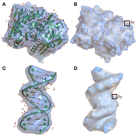
Figure 4. Top (A,B): Gaussian map of the protein and Bottom (C,D): of the DNA dodecamer. (A,C) highlights smoothed Gaussian mapping of the macromolecules, at 5 Å resolution, indicating crystallographic distribution of the water molecules on the surface. (B,D) shows the mapping of the macromolecules at two different resolutions, capturing surface thickness variation incorporated in δρ. Blue surface is mapping at 2 Å resolution and indicates distribution of the atoms on the surface, while light gray is the smoothed Gaussian map indicating how surface thickness may vary if free diffusion of the solvent molecules on the surface is taken into account.

Let's model a bio-macromolecular surface as a Gaussian map contoured at 2 Å to 8 Å resolution. Figure 4 shows Gaussian maps for the protein (Figures 4A,B) and for the DNA (Figures 4C,D). Ω is the space inside the macromolecules and the boundary of the space is the surface S. S_i base vectors are defined in the tangent space of the Gaussian map. S_ij is the metric tensor of the map. These are illustrations of surfaces as two-manifolds embedded in Euclidian space and are only true for non-relativistic representations, therefore they do not show the shape of three-manifolds in Minkowski space-time. Figures 4A,C show a Gaussian map of the polypeptide main chain of a protein and of a polynucleotide double helical DNA dodecamer, respectively¹². Figures 4B,D show thickness variations, captured by surface mass density, of the modeled surfaces for the protein and DNA. Light gray is the Gaussian map at 5 Å resolution while the blue surface indicates a more detailed surface contoured at 2 Å resolution. Thickness variation can be induced by diffusion of solvent molecules at solvent accessible sites; e.g., sites marked by water molecules obtained from crystal structures as illustrated in the Figures 4A,C (red and white sticks), or by thermal fluctuation of amino acid sidechains. In all these cases, the surface thickness variation, captured by ρ surface mass density, is in the range of angstrom to nanometer. This range is higher for micelles, cell membranes, fluid films etc. If the system is in aqueous solution then the surface motion is determined by so called hydrophobic-hydrophilic interactions.

As we already stated in the introduction, hydrophobic and hydrophilic interactions incorporate dispersive interactions throughout the molecules, mainly related to electrostatics and electrodynamics (Van der Waals forces), induced by permanent (water molecules) or induced dipoles (dipole-dipole interactions) and possibly quadrupole-quadrupole interactions (for instance stacking or London forces) plus ionic interactions (Coulomb forces) [20]. The hydrophobic effect can be considered as synonymous with dispersive interactivity with water molecules and the hydrophilic one as synonymous with polar interactivity with water molecules [14, 19, 20]. All these interactions have one common feature and can be unified as electromagnetic interaction's dependence on interacting bodies' geometries, where by geometries we mean shape of the objects' surfaces. To model potential energy we note that on the scale of hydrophobic-hydrophilic interactions, which usually occurs at nanometer distances [19, 20], no interactions other than electromagnetic forces are available. An electromagnetic field is set up by dipole moments of water molecules and partial charges of molecules. In other words, we have a closed, smooth manifold in aqueous solution where charge and water molecules could migrate through the surface Figure 4. The surface can be of mixed nature (hydrophobic, hydrophilic, or both) with randomly distributed polar or non-polar groups and can be compressible, continuously deformable and permeable against water and ionic charges. At the nanometer scale, for small masses, potential energy can be electromagnetic only. Therefore, we have potential energy density constructed from the electromagnetic tensor plus the term related to variation of charges as it is defined in (27). Even though modeling of potential energy as electromagnetic interaction energy is fairly clear, the dependence of these interactions on the object's geometry is not. The geometry dependence becomes visible only after the complete formulation of the equations of motion (53).

4. Results and Discussions

4.1. Poisson-Boltzmann Equation

To demonstrate effectiveness of (53) let's discuss free motion of two manifolds embedded in three dimensional Euclidean space for the stationary surface in an electrostatic field. We have the following conditions: V = 0 stationary surface in electrostatic field where a = 0, j = 0, A_· = (−φ/c, 0), J^· = (cQ, 0) and ∂ = (0, ∂_x, ∂_y, ∂_z). Then from second equation of (53) with the condition (46), we find

$\begin{array}{cc}cQ-\frac{1}{{\mu }_0}{\partial }_{\beta }{F}^{\beta 0}=0& (56)\end{array}$

Taking into account the definition of electromagnetic tensor and that we consider the electrostatic field, the partial derivative of the electromagnetic tensor in (56) is $(1/c){\partial }_{\beta }{E}^{\beta }$ and therefore

$\begin{array}{cc}{\partial }_{\beta }{E}^{\beta }=c^2{\mu }_{0}Q& (57)\end{array}$

By the definition of the electric field E^β = −∂^βφ and $c^2{\mu }_0=1/{ϵ}_0$ so that (57) transforms to

$\begin{array}{cc}{\partial }_{\alpha }{\partial }^{\alpha }\phi ={\nabla }^2\phi =-\frac{Q}{{ϵ}_0}& (58)\end{array}$

The equation (58) is generally known as the Poisson-Boltzmann equation in vacuum and was proposed to describe the distribution of the electric potential in the direction of the normal to a charged surface [34–36].

Here we demonstrate that the Poisson-Boltzmann equation is a special case and can be obtained from the equations of motion (53) for stationary surfaces in an electrostatic field. To support this statement we have generated electrostatic field lines using the Adaptive Poisson-Boltzmann Solver (APBS) [37] software for the protein [32] and the DNA [33] (Figure 5). As can be seen from Figure 5 field lines follow the surface normal as expected from the second equation of (53) for the V = 0 stationary case.

FIGURE 5

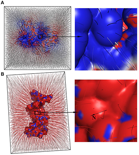
Figure 5. Color-coded electrostatic surface where red indicates negatively charged regions of the surface, white neutrally charged and blue positively charged one. Simulated electrostatic field lines are displayed as hairs on the surface of the protein (A) and the DNA (B). Hairs are generated by the adaptive Poisson-Boltzmann solver and highlight how variations of the field lines on the surface describe the charge distribution pattern on the surface. The right side of the figure shows the position of the surface normal N and electrostatic hairs.

4.2. Classical Electrodynamics, Maxwell Equations

In this subsection we demonstrate that, the equations of motion simplify to Maxwell equations for stationary interfaces C = 0 and massless ρ = 0 three manifolds embedded in Minkowski space. Indeed, from the second and the third equations of (53), taking into account that in the stationary case the second term in (32) vanishes, we find

$\begin{array}{cc}{\displaystyle {\int }_{\Omega }{F}}{A}d\Omega =0& (59)\end{array}$

$\begin{array}{cc}{\displaystyle {\int }_{\Omega }{{F}}^i}{{A}}_{i}d\Omega =0& (60)\end{array}$

Adding (59) to (60) and taking into account (47) and (49) one obtains

$\begin{array}{cc}{F}{A}+{{F}}^i{{A}}_i={F}·\frac{\partial A}{\partial t}=0& (61)\end{array}$

(61) must hold for any partial time derivative of the four vector potential, therefore

$\begin{array}{cc}{F}=({{F}}^{\alpha })=(J^{\alpha }-\frac{1}{{\mu }_0}{\partial }_{\beta }{F}^{\beta \alpha })=0& (62)\end{array}$

and the Maxwell equations with the source in the vacuum follow.

$\frac{1}{{\mu }_0}{\partial }_{\beta }{F}^{\beta \alpha }=J^{\alpha }$

This is a somewhat unexpected result: any three manifold with stationary interface C = 0 and with massless surface mass density ρ = 0¹³, satisfies Maxwell equations. However, the photon is arguably the only massless particle that satisfies the Maxwell equation, therefore the photon can be interpreted as a stationary interface three manifold embedded in Minkowski space with vanishing surface mass density.

4.3. Classical Hydrodynamics, Euler Equation

In this section we simplify the equations of motion using physical arguments and demonstrate that the equation system (53) yields the Euler equation for a dynamic fluid for some simplified cases. Let's propose that a moving fluid has a planar surface B_ij = 0 with stationary interface C = 0 and is embedded in Euclidean three space. Then simplifications of (53) lead to a system of equations of motion

$\begin{array}{cc}\begin{array}{l}\dot{\nabla }\rho +{\nabla }_i(\rho V^i)=0\\ {F}{A}=0\\ {\displaystyle {\int }_S\rho }{V}_i(\dot{\nabla }{V}^i+V^j{\nabla }_j{V}^i)dS={\displaystyle {\int }_{\Omega }{{F}}^i}{{A}}_{i}d\Omega \end{array}& (63)\end{array}$

The first equation of (63) is the continuity equation for the surface mass density and is conservation of mass at the flat space; the second one yields that normal component of the dot product ${F}$ · (∂A/∂t) vanishes. To simplify the last equation of (63) we note that the total 'force' acting on the volume is equal to the integral $-{\int }_{S}pdS$ of the total pressure p, taken over the boundary (surface) of the volume. Applying Gauss' theorem to the surface integral by taking into account that pressure across the surface acts in a normal direction so that it can be written as $p=p_{\alpha }{N}^{\alpha }$, then

$\begin{array}{cc}-{\displaystyle {\int }_{S}p}dS=-{\displaystyle {\int }_S{p}_{\alpha }}{N}^{\alpha }dS=-{\displaystyle {\int }_{\Omega }{\nabla }^{\alpha }}{p}_{\alpha }d\Omega & (64)\end{array}$

On the other hand ${{F}}^i{{A}}_i$ is a cause of the gradient of the tangential velocity and the tangential gradient of the pressure, therefore

$\begin{array}{cc}{{F}}^i{{A}}_i=-{\nabla }^{\alpha }(V_i{\nabla }^i{p}_{\alpha })& (65)\end{array}$

Taking into consideration (64, 65) in (63) and applying Gauss' theorem to the space integral, we find

$\begin{array}{cc}\begin{array}{l}{\displaystyle {\int }_S\rho }{V}_i(\dot{\nabla }{V}^i+V^j{\nabla }_j{V}^i)dS={\displaystyle {\int }_{\Omega }{{F}}^i}{{A}}_{i}d\Omega \\ =-{\displaystyle {\int }_{\Omega }{\nabla }^{\alpha }}(V_i{\nabla }^i{p}_{\alpha })d\Omega \\ =-{\displaystyle {\int }_S{V}_i}{N}^{\alpha }{\nabla }^i{p}_{\alpha }dS\end{array}& (66)\end{array}$

According to Weingarten's formula (24) N^α is invariant vs the surface derivative for flat manifolds and therefore, can be taken into the surface covariant derivative, so that $V_i{N}^{\alpha }{\nabla }^i{p}_{\alpha }=V_i{\nabla }^{i}p$¹⁴. Then (66) after subtracting V_i yields

$\begin{array}{cc}\rho (\dot{\nabla }{V}^i+V^j{\nabla }_j{V}^i)=-{\nabla }^{i}p& (67)\end{array}$

Taking into account that for flat surfaces Christoffel symbols vanish and ∇_j = ∂_j one immediately recognizes that the last equation (67) becomes the classical Euler equation of fluid dynamics.

As stated above the equations of motion (53) are formulated for freely moving manifolds; i.e., interaction with the environment is ignored and matter is set to be a vacuum. Though it can be trivially generalized for the matter and then simplified, instead of giving Euler equation, will lead to the more complete Navier-Stokes equation and or magnetohydrodynamic equations. For instance, in matter, according to (55), the electromagnetic tensor becomes the sum of the electric displacement and magnetization tensors. Therefore, in (67), instead of a pure pressure gradient we will have an additive term coming from the magnetic field so that (67) will transform to the ideal magneto hydrodynamic equation.

Analogously, if interaction with an environment is taken into account, then instead of a single surface we have two surfaces at the surface/environment interface and the Lagrangian (30) is split into two kinetic energy terms, one for surface and another one for the environmental interface. All these will occur as additive terms in the third equation of (53) so that equation (67) will transform to the Navier-Stokes equation.

4.4. Equilibrium Shapes of Micelles

Let's answer the question: what is the shape of micelles formed from lipid molecules when they are in thermodynamic equilibrium with solvent. Lipids have hydrophilic heads and hydrophobic tails, so that in solutions they tend to form a surface with heads on one side and tails on the other. Since the tails disperse the water molecules, the surface made is closed and has some given volume. Such structures are called micelles [38]. Since lipids form a homogeneous surface, in equilibrium conditions we must have

$\begin{array}{cc}{F}{A}=const\ne 0& (68)\end{array}$

and ${{F}}^i{{A}}_i=0$. Usually the speed of micelle interface motion is in the range of nm/ns and, therefore there is no necessity of discussion of a relativistic formalism so that the surface is two dimensional and the space is Euclidean. The surface dynamic is slow, magnetic field is much smaller then electric field B² < < E² and the potential energy becomes

$\begin{array}{cc}{U}=-{\displaystyle {\int }_{\Omega }(\frac{{ϵ}_0}{2}{E}^2+\phi Q)}d\Omega & (69)\end{array}$

Using the first law of thermodynamics, (69) can be modeled as a volume integral from the surface pressure [28] and

$\begin{array}{cc}p=\frac{{ϵ}_0}{2}{E}^2+\phi Q& (70)\end{array}$

On the other hand, taking into account the conditions (68, 69), the total potential energy of the surface can be modeled as

$\begin{array}{cc}{U}=\sigma {\displaystyle {\int }_{S}d}S& (71)\end{array}$

Taking into account (71), the system Lagrangian becomes the same as it is in (1) and its variation leads to the equation

$\begin{array}{cc}\rho (\dot{\nabla }C+2V^i{\nabla }_{i}C+V^i{V}^j{B}_{ij})=\sigma B_i^i& (72)\end{array}$

(72) was first reported in Grinfeld [10]. Using (69, 70, 72) in the equations of motion (53), after simple algebra we find

$\begin{array}{cc}{\partial }_{\alpha }(\sigma V^{\alpha }{B}_i^i+p{V}^{\alpha })=-V^{\alpha }{\partial }_{\alpha }p& (73)\end{array}$

When the homogeneous surface, such as a micelle, is in equilibrium with the environment then the solution of the (73)¹⁵ is

$\begin{array}{cc}{B}_i^i=-\frac{p}{\sigma }& (74)\end{array}$

From equation (74) the generalized Young-Laplace relation which connects the surface pressure to the curvature and the surface tension immediately follows. (74) dictates that the homogeneous surfaces in equilibrium with environment adopt a shape with constant mean curvatures (CMC), which explains the well anticipated lamellar, cylindrical and spherical shapes of micelles. This is another unexpected and surprisingly simple solution to the equations of motion (53).

4.5. Motion of Two Surfaces

Equations of motion (53) further simplify for two dimensional surfaces. In non-relativistic framework the space is three dimensional Euclidean (α = 1, 2, 3 and V⁰ = 0 limit), the surface is two-dimensional Riemannian (i = 1, 2) and the potential energy becomes

$\begin{array}{cc}{U}={\displaystyle {\int }_{\Omega }(-\frac{{ϵ}_0}{2}{E}^2+\frac{1}{2{\mu }_0}{B}^2-\phi Q+\mathbf{a}\mathbf{j})}d\Omega & (75)\end{array}$

where E, B are electric and magnetic fields and φ, Q, a, j are charge density, electric potential, magnetic vector potential and current density vector respectively. Using same formalism as in (65, 66, 69, 70) into account we find

$\begin{array}{cc}{F}{A}=-V^{\alpha }{\partial }_{\alpha }p& (76)\end{array}$

$\begin{array}{cc}{\displaystyle {\int }_{\Omega }{{F}}_i}{{A}}^{i}d\Omega =-{\displaystyle {\int }_S{V}_j}{N}^{\alpha }{\nabla }^j{p}_{\alpha }dS& (77)\end{array}$

Taking (76, 77) along with that $p=\frac{{ϵ}_0}{2}{E}^2-\frac{1}{2{\mu }_0}{B}^2+\phi Q-\mathbf{a}\mathbf{j}$ into account we end up with the following equations of motion for two dimensional surfaces:

$\begin{array}{cc}\dot{\nabla }\rho +{\nabla }_i(\rho V^i)=\rho C{B}_i^i& (78)\end{array}$

$\begin{array}{cc}{\partial }_{\mu }(V^{\mu }(\rho (\dot{\nabla }C+2V^i{\nabla }_{i}C+V^i{V}^j{B}_{ij})+p))=-V^{\alpha }{\partial }_{\alpha }p& (79)\end{array}$

$\begin{array}{cc}\rho V_i(\dot{\nabla }{V}^i+V^j{\nabla }_j{V}^i-C{\nabla }^{i}C-C{V}^j{B}_j^i)=-V_j{N}^{\alpha }{\nabla }^j{p}_{\alpha }& (80)\end{array}$

Alternative way of deducing (78–80) without using (53) is given in Svintradze [28]. In equations of motions for two dimensional surfaces (78–80) we mention that only first equation (78) is the same as dynamic fluid film equations [10]. (78) captures surface mass density variation during the manifold motion, second equations (79) shows how the surface moves in normal direction and third equation (80) shows how the surface moves in tangent directions. Soup films, water droplets and for all two dimensional surfaces which satisfies preconditions: (1) the surface is homogeneous, (2) surface potential energy density σ is time invariable, and (3) the surface is in thermodynamic equilibrium with environment can be solved exactly the same way as it is done in sub-section 4.4 with the solution (74).

5. Conclusions

We have proposed equations of moving surfaces in an electromagnetic field and demonstrated that the equations simplify to: (1) Maxwell equations for massless three manifolds with stationary interfaces; (2) Euler equations for dynamic fluid for planar two manifolds with stationary interface embedded in Euclidean space, which can be generalized to Navier-Stokes equations and to magneto-hydrodynamic equations; (3) Poisson-Boltzmann equation for stationary surfaces in electrostatic field.

We have applied the equation to analyze the motion of hydrophobic-hydrophilic surfaces and explained “equilibrium” shapes of micelles. Analyses were in good qualitative as well as quantitative agreement with known experimental results for micelles [28]. Analytic solutions to simplified equations for homogeneous surfaces in equilibrium with the environment produced generalized the Young-Laplace law and explained why mean curvature surfaces are such abundant shapes in nature.

Also we have shown that hydrophobic-hydrophilic effects are just another expression of well known electromagnetic interactions. In particular, equations of motion for moving surfaces in hydrophobic and hydrophilic interactions, together with the analytic solution, provide an explanation for the nature of the hydrophobic-hydrophilic effect. Hydrophobic and hydrophilic interactions are dispersive interactions throughout the molecules and conform to electromagnetic interaction dependence on surface morphology of the material bodies.

Author Contributions

The author confirms being the sole contributor of this work and approved it for publication.

Conflict of Interest Statement

The author declares that the research was conducted in the absence of any commercial or financial relationships that could be construed as a potential conflict of interest.

Acknowledgments

We were partially supported by personal savings accumulated during the visits to Department of Mechanical Engineering, Department of Chemical Engineering, OCMB Philips Institute and Institute for Structural Biology and Drug Discovery of Virginia Commonwealth University in 2007–2012 years. We thank Dr. Alexander Y. Grosberg from New York University for comments on an early draft of the paper and Dr. H. Tonie Wright from Virginia Commonwealth University for editing the English. Limited access to Virginia Commonwealth University's library in 2012–2013 years is also gratefully acknowledged.

Footnotes

1. ^If one proposes to treat particles as classical objects, then the framework fits in Newtonian mechanics. The application of Newton laws and it's stochastic generalizations in simulations is commonly known as molecular dynamics simulations.

2. ^e.g., bio-membranes, macromolecular surfaces, lipid bilayers, micelles, etc.

3. ^The formalism should be relativistic not only because relativistic calculations are more general than classical calculations, or because a proper electrodynamics description requires a relativistic frame work, but also because molecular surface dynamics can be very fast [11, 12].

4. ^Here the speed of light is set to be unit c = 1 and i stands for imaginary number.

5. ^Proofs for the time derivative of integrals can be found in tensor calculus text books. See for instance [26] and references therein.

6. ^same explanation, with more details, is given in Svintradze [28].

7. ^Details about the proof for Euclidean space can be found in tensor calculus text book [26] and proof for Minkowski space is identical to Euclidean one.

8. ^The environment is set to be vacuum.

9. ^In the case of taking into account interaction with the environment we no longer have single surface. Instead there are double surfaces where one is the boundary of the material body and another one is the surface of the environment at the boundary/environment interface. Having two surfaces raises the terms related to surface-surface interactions and may enter into final equations as a viscoelastic effect incorporated in coefficient of viscosity.

10. ^Or surface made from groups of molecules, for instance lipids.

11. ^Especially for relatively slowly moving surfaces, for instance: cell surface, which is bio-membrane; vesicles; micelles etc.

12. ^The model protein is the peroxide sensitive gene regulator with Protein Data Bank (PDB) ID 3HO7 [32]. The model DNA is the double helical dodecamer generally known as library DNA with PDB ID 1BNA [33].

13. ^Here surface mass density is the same as the mass density of the three manifold, because the three manifold is the surface in 4D space.

14. ^More information about how the term ${F}$·∂A/∂t can be modeled as gradient of pressure times velocity can be found in Svintradze [28].

15. ^A shorter alternative way to deduce (73) and it's solution in equlibrium conditions is given in Svintradze [28].

References

1. Landau LD, Lifshitz EM. Fluid Mechanics. London: Pergamon Press (1959).

2. Seifert U. Configurations of fluid membranes and vesicles. Adv Phys. (1997) 46:13–137.

Google Scholar

3. Lipowsky R, Sackmann E. Structure and Dynamics of Membranes. Amsterdam: Elsevier (1995).

Google Scholar

4. Drenckhan W, Dollet B, Hutzler S, Elias F. Soap films under large-amplitude oscillations. Philos Mag Lett. (2008) 88:669–77. doi: 10.1080/09500830802220125

CrossRef Full Text | Google Scholar

5. Brazovskaia M, Dumoulin H, Pieranski P. Nonlinear effects in vibrating smectic films. Phys Rev Lett. (1996) 76:1655–8. doi: 10.1103/PhysRevLett.76.1655

PubMed Abstract | CrossRef Full Text | Google Scholar

6. Kraus I, Bahr C, Chikina IV, Pieranski P. Can one hear structures of smectic films? Phys Rev E (1998) 58:610–25. doi: 10.1103/PhysRevE.58.610

CrossRef Full Text | Google Scholar

7. Seychelles F, Amarouchene Y, Bessafi M, Kellay H. Thermal convection and emergence of isolated vortices in soap bubbles. Phys Rev Lett. (2008) 100:144501. doi: 10.1103/PhysRevLett.100.144501

PubMed Abstract | CrossRef Full Text | Google Scholar

8. Grinfeld P. Variable thickness model for fluid films under large displacement. Phys Rev Lett. (2010) 105:137802. doi: 10.1103/PhysRevLett.105.137802

CrossRef Full Text | Google Scholar

9. Manor O, Rezk AR, Friend JR, Yeo LY. Dynamics of liquid films exposed to high-frequency surface vibration. Phys Rev E Stat Nonlin Soft Matter Phys. (2015) 91:053015. doi: 10.1103/PhysRevE.91.053015

PubMed Abstract | CrossRef Full Text | Google Scholar

10. Grinfeld P. Exact nonlinear equations for fluid films and proper adaptations of conservation theorems from classical hydrodynamics. J Geom Symmetry Phys. (2009) 16:1–21.

Google Scholar

11. Pal SK, Peon J, Bagchi B, Zewail AH. Biological water: femtosecond dynamics of macromolecular hydration. J Phys Chem B (2002) 106:12376–95. doi: 10.1021/jp0213506

CrossRef Full Text | Google Scholar

12. Wan C, Fiebig T, Schiemann O, Barton JK, Zewail AH. Femtosecond direct observation of charge transfer between bases in DNA. Proc Natl Acad Sci USA. (2000) 97:14052–5. doi: 10.1073/pnas.250483297

PubMed Abstract | CrossRef Full Text | Google Scholar

13. Lum K, Chandler D, Weeks JD. Hydrophobicity at small and large length scales. J Phys Chem B. (1999) 103:4570–7.

Google Scholar

14. Chandler D, Garrahan JP. Dynamics on the way to forming glass: bubbles in space-time. Ann Rev Phys Chem. (2010) 61:191–217. doi: 10.1146/annurev.physchem.040808.090405

PubMed Abstract | CrossRef Full Text | Google Scholar

15. Patel AJ, Varilly P, Jamadagni SN, Acharya H, Garde S, Chandler D. Extended surfaces modulate hydrophobic interactions of neighboring solutes. Proc Natl Acad Sci USA. (2011) 108:17678–83. doi: 10.1073/pnas.1110703108

PubMed Abstract | CrossRef Full Text | Google Scholar

16. Rotenberg B, Patel AJ, Chandler D. Molecular explanation for why talc surfaces can be both hydrophilic and hydrophobic. J Am Chem Soc. (2011) 133:20521–7. doi: 10.1021/ja208687a

PubMed Abstract | CrossRef Full Text | Google Scholar

17. Patel AJ, Varilly P, Jamadagni SN, Hagan MF, Chandler D, Garde S. Sitting at the edge: how biomolecules use hydrophobicity to tune their interactions and function. J Phys Chem B (2012) 116:2498–503. doi: 10.1021/jp2107523

PubMed Abstract | CrossRef Full Text | Google Scholar

18. Limmer DT, Merlet C, Salanne M, Chandler D, Madden PA, van Roij R, et al. Charge fluctuations in nanoscale capacitors. Phys Rev Lett. (2013) 111:106102. doi: 10.1103/PhysRevLett.111.106102

PubMed Abstract | CrossRef Full Text | Google Scholar

19. Chandler D. Interfaces and the driving force of hydrophobic assembly. Nature (2005) 437:640–7. doi: 10.1038/nature04162

CrossRef Full Text | Google Scholar

20. Leikin S, Parsegian VA, Rau DC, Rand RP. Hydration forces. Annu Rev Phys Chem. (1993) 44:369–95.

PubMed Abstract | Google Scholar

21. Svintradze DV. Hydrophobic and hydrophilic interactions. Biophys J. (2010) 98:43a–44a. doi: 10.1016/j.bpj.2009.12.250

CrossRef Full Text | Google Scholar

22. Svintradze DV. Moving macromolecular surfaces under hydrophobic/hydrophilic stress. Biophys J. (2015) 108:512a. doi: 10.1016/j.bpj.2014.11.2807

CrossRef Full Text | Google Scholar

23. Svintradze DV. Predictive power of conformational motion. Biophys J. (2013) 104:68a–9a. doi: 10.1016/j.bpj.2012.11.415

CrossRef Full Text | Google Scholar

24. Svintradze DV. Conformational motion of biological macromolecules. Biophys J. (2009) 96:584a–5a. doi: 10.1016/j.bpj.2008.12.3058

CrossRef Full Text | Google Scholar

25. Vanderlinde J. Classical Electromagnetic Theory. New York, NY: Springer (2004).

Google Scholar

26. Grinfeld P. Introduction to Tensor Analysis and the Calculus of Moving Surfaces. New York, NY: Springer (2013).

Google Scholar

27. Weyl H. Space, Time, Matter. New York, NY: Dover Publications (1952).

28. Svintradze D. V. Micelles hydrodynamics. arXiv preprint arXiv:1608.01491 [physics.bio-ph]. (2016).

Google Scholar

29. Landau LD, Lifshitz EM. The Classical Theory of Fields. London: Pergamon Press (1971).

Google Scholar

30. Hadamard J. Mmoire Sur le Problme Danalyse Relatif Lquilibre des Plaques Elastiques Encastres. Oeuvres, Hermann, Tome 2 (1968).

31. Johns OD. Analytical Mechanics for Relativity and Quantum Mechanics. New York, NY: Oxford University Press Inc (2005).

Google Scholar

32. Svintradze DV, Peterson DL, Collazo-Santiago EA, Lewis JP, Wright HT. Structures of the Porphyromonas gingivalis OxyR regulatory domain explain differences in expression of the OxyR regulon in Escherichia coli and P. gingivalis. Acta Crystallogr Sec D Biol Crystallogr. (2013) 69:2091–103. doi: 10.1107/S0907444913019471

PubMed Abstract | CrossRef Full Text | Google Scholar

33. Drew HR, Wing RM, Takano T, Broka C, Tanaka S, Itakura K, et al. Structure of a B-DNA dodecamer: conformation and dynamics. Proc Natl Acad Sci USA. (1981) 78:2179–83.

PubMed Abstract | Google Scholar

34. Gouy M. Sur la constitution de la charge electrique a la surface d'un electrolyte. J Phys Theor Appl. (1910) 9:457–68.

Google Scholar

35. Chapman DL. LI. A contribution to the theory of electrocapillarity. Philos Mag. (1913) 25:475–81.

Google Scholar

36. Davis ME, McCammon JA. Electrostatics in biomolecular structure and dynamics. Chem Rev. (1990) 90:509–21.

Google Scholar

37. Dolinsky TJ, Czodrowski P, Li H, Nielsen JE, Jensen JH, Klebe G, et al. PDB2PQR: expanding and upgrading automated preparation of biomolecular structures for molecular simulations. Nucleic Acids Res. (2007) 35(Suppl. 2):W522–5. doi: 10.1093/nar/gkm276

PubMed Abstract | CrossRef Full Text | Google Scholar

38. Tanford C. The Hydrophobic Effect Formation of Micelles and Biological Membranes. New York, NY: Wiley-Interscience (1973).

Google Scholar