Status of Neutrino Properties and Future Prospects—Cosmological and Astrophysical Constraints

1. Introduction

Flavor oscillation experiments have by now firmly established that neutrinos have a mass. Current experiments measure with great accuracy the three mixing angles, as well as the two mass-squared splittings between the three active neutrinos. In the framework of the standard model (SM) of particle physics neutrinos are massless, and consequently do not mix, since it is not possible to build a mass term for them using the particle content of the SM. Therefore, flavor oscillations represent the only laboratory evidence for physics beyond the SM. Several unknowns in the neutrino sector still remain, confirming these particles as being the most elusive within the SM. In particular, the absolute scale of neutrino masses has yet to be determined. Moreover, the sign of the largest mass squared splitting, the one governing atmospheric transitions, is still unknown. This leaves open two possibilities for the neutrino mass ordering, corresponding to the two signs of the atmospheric splitting: the normal hierarchy, in which the atmospheric splitting is positive, and the inverted hierarchy, in which it is negative. Other unknowns are the value of a possible CP-violating phase in the neutrino mixing matrix, and the Dirac or Majorana nature of neutrinos.

There are different ways of measuring the absolute neutrino mass scale. One is to use kinematic effects, for example by measuring the energy spectrum of electrons produced in the β-decay of nuclei, looking for the distortions due to the finite neutrino mass. This approach has the advantage of being very robust and providing model-independent results, as it basically relies only on energy conservation. Present constraints on the effective mass of the electron neutrino m_β (an incoherent sum of the mass eigenvalues, weighted with the elements of the mixing matrix) are m_β < 2.05 eV from the Troitsk [1] experiment, and m_β < 2.3 eV from the Mainz [2] experiment, at the 95% CL. The KATRIN spectrometer [3], that will start its science run in 2018, is expected to improve the sensitivity by an order of magnitude. Another way to measure neutrino masses in the laboratory is to look for neutrinoless double β decay (0ν2β in short) of nuclei, a rare process that is allowed only if neutrinos are Majorana particles [4]. The prospects for detection of neutrino mass with 0ν2β searches are very promising: current constraints for the effective Majorana mass of the electron neutrino m_ββ, a coherent sum of the mass eigenvalues, weighted with the elements of the mixing matrix, are in the m_ββ < 0.1 ÷ 0.4 eV ballpark (see section 9 for more details). There are a few shortcomings, however. First of all, there is some amount of model dependence: one has to assume that neutrinos are Majorana particles to start, and even if this is, in some sense, a natural and very appealing scenario from the theoretical point of view—as it could explain the smallness of neutrino masses [5–9]—we have at the moment no indication that this is really the case. Moreover, inferring the neutrino mass from a (non-)observation of 0ν2β requires the implicit assumption that the mass mechanism is the only contribution to the amplitude of the process, i.e., that no other physics beyond the SM that violates lepton number is at play. Another issue is that the amplitude of the process also depends on nuclear matrix elements, that are known only with limited accuracy, introducing an additional layer of uncertainty in the interpretation of experimental results. Finally, given that m_ββ is a coherent superposition of the mass eigenvalues, it could be that the values of the Majorana phases arrange to make m_ββ vanishingly small.

The third avenue to measure neutrino masses, and in fact the topic of this review, is to use cosmological observations. As we shall discuss in more detail in the following, the presence of a cosmic background of relic neutrinos (CνB) is a robust prediction of the standard cosmological model [10]. Even though a direct detection is extremely difficult and still lacking, (but experiments aiming at this are currently under development, like the PTOLEMY experiment [11]), nevertheless cosmological observations are in agreement with this prediction. The relic neutrinos affect the cosmological evolution, both at the background and perturbation level, so that cosmological observables can be used to constrain the neutrino properties, and in particular their mass (see e.g., [10, 12, 13] for excellent reviews on this topic). In fact, cosmology currently represents the most sensitive probe of neutrino masses. The observations of cosmic microwave background (CMB) anisotropies from the Planck satellite, without the addition of any external data, constrain the sum of neutrino masses already at the 0.6 eV level [14], which is basically the same as the KATRIN sensitivity. Combinations of different datasets yield even stronger limits, at the same level or better than the ones from 0ν2β searches, although a direct comparison is not immediate, due to the fact that different quantities are probed, and also due to the theoretical assumptions involved in the interpretation of both kinds of data. Future-generation experiments will likely have the capability to detect neutrino masses, and to disentangle the hierarchy, provided that systematics effects can be kept under control—and that our theoretical understanding of the Universe is correct, of course! Concerning this last point, the drawback of cosmological measurements of neutrino mass and other properties, is that they are somehow model dependent. Inferences from cosmological observations are made in the framework of a model—the so-called ΛCDM model—, and of its simple extensions, that currently represents our best and simple description of the Universe that is compatible with observations. This model is based on General Relativity (with the assumption of a homogeneous and isotropic Universe at large scales) and on the SM of particle physics, with the addition of massive neutrinos, complemented with a mechanism for the generation of primordial perturbations, i.e., the inflationary paradigm. When cosmological data are interpreted in this framework, they point to the following picture: our Universe is spatially flat and is presently composed by baryons (~5% of the total density), dark matter (~25%), and an even more elusive component called dark energy (~70%), that behaves like a cosmological constant, and is responsible for the present accelerated expansion, plus photons (a few parts in 10⁵) and light neutrinos. The constraints from Planck cited above imply that, in the framework of the ΛCDM model, neutrinos can contribute 1% to the present energy density at most. The structures that we observe today have evolved from adiabatic, nearly scale-invariant initial conditions. Even though this model is very successful, barring some intriguing but for the moment still mild (at the ~2σ level) discrepancies between observational probes, this dependence should be borne in mind. On the other hand, such a healthy approach should not, in our opinion, be substituted with its contrary, i.e., a complete distrust toward cosmological constraints. A pragmatic approach to this problem is to test the robustness of our inferences concerning neutrino properties against different assumptions, by exploring extensions of the ΛCDM model. This has been in fact done quite extensively in the literature, and we will take care, toward the end of the review, to report results obtained in extended models.

Another advantage of cosmological observations is that they are able to probe neutrino properties beyond their mass. A well-known example is the effective number of neutrinos, basically a measure of the energy density in relativistic species in the early Universe, that is a powerful probe of a wide range of beyond the SM model physics (in fact, not necessarily related to neutrinos). For example, it could probe the existence of an additional, light sterile mass eigenstate, as well as the physics of neutrino decoupling, or the presence of lepton asymmetries generated in the early Universe. Cosmology can also be used to constrain the existence of non-standard neutrino interactions, possibly related to the mechanism of mass generation. Even though they are not the focus of this review, we will briefly touch some of these aspects in the final sections of the review.

Cosmological data have reached a very good level of maturity over the last decades. Measurements of the CMB anisotropies from the Planck satellite have put the tightest constraints ever on cosmological parameters from a single experiment [14], dramatically improving the constraints from the predecessor satellite WMAP [15]. From the ground, the Atacama Cosmology Telescope (ACT) polarization-sensitive receiver and the South Pole Telescope (SPT) have been measuring with incredible accuracy CMB anisotropies at the smallest scales in temperature and polarization [16, 17]. At degree and sub-degree scales, the BICEP/Keck collaboration [18, 19] and the POLARBEAR telescope [20] are looking at the faint CMB “B-mode” signal, containing information about both the early stages of the Universe (primordial B-modes) and the late time evolution (lensing B-modes). The Cosmology Large Angular Scale Surveyor (CLASS) [21] is working at mapping the CMB polarization field over 70% of the sky. The SPIDER balloon [22] successfully completed its first flight and is in preparation for the second launch likely at the end of 2018. In addition to CMB data, complementary information can be obtained by looking at the large-scale structure of the Universe. The SDSS III-BOSS galaxy survey has recently released its last season of data [23]. Extended catalogs of galaxy clusters have been completed from several surveys (see e.g., [24] and references therein). In addition, weak lensing surveys (Canada-France-Hawaii Telescope Lensing Survey [25], Kilo-Degree Survey [26], Dark Energy Survey [27]) are mature enough to provide constraints on cosmological parameters that are competitive with those from other observables. They also allow to test the validity of the standard cosmological paradigm by comparing results obtained from high-redshift observables to those coming from measurements of the low-redshift universe.

The current scenario is just a taste of the constraining power of cosmological observables that will be available with the next generation of experiments, that will be taking measurements in the next decade. Future CMB missions—including Advanced ACTPol [28], SPT-3G [29], CMB Stage-IV [30], Simons Observatory¹, Simons Array [31], CORE [32], LiteBIRD [33], PIXIE [34]—will test the Universe over a wide range of scales with unprecedented accuracy. The same accuracy will enable the reconstruction of the weak lensing signal from the CMB maps down to the smallest scales and with high sensitivity, providing an additional probe of the distribution and evolution of structures in the universe. On the other hand, the new generation of large-scale-structure surveys—including the Dark Energy Spectroscopic Instrument [35], the Large Synoptic Survey Telescope [36], Euclid [37], and the Wide Frequency InfraRed Spectroscopic Telescope [38]—will also probe the late-time universe with the ultimate goal of shedding light on the biggest unknown of our times, namely the nature of dark energy and dark matter.

The aim of this review is to provide the state of the art of the current knowledge of neutrino masses from cosmological probes and give an overview of future prospects. The review is organized as follows: in section 2, we outline the framework of this review, introducing some useful notation and briefly reviewing the basics of neutrino cosmology. Section 3 is devoted to discussing, from a broad perspective, cosmological effects induced by massive neutrinos. In section 4, we will describe in detail how the effects introduced in section 3 affect cosmological observables, such as the CMB anisotropies, large-scale structures and cosmological distances. Sections 5 and 6 present a detailed collection of the current and future limits on Σm_ν from the measurements of the cosmological observables discussed in section 4, mostly derived in the context of the ΛCDM cosmological model. Constraints derived in more extended scenarios are summarized in section 7. Section 8 briefly deals with the issue of whether cosmological probes are able to provide information not only on Σm_ν, but also on its distribution among the mass eigenstates, i.e., about the neutrino hierarchy. In section 9, we will briefly go through the complementarity between cosmology and laboratory searches in the quest for constraining neutrino properties. Finally, section 10 offers a summary of the additional information about neutrino properties beyond their mass scale that we can extract from cosmological observables. We derive our conclusions in section 11. The impatient reader can access the summary of current and future limits from Tables 1–4.

TABLE 1

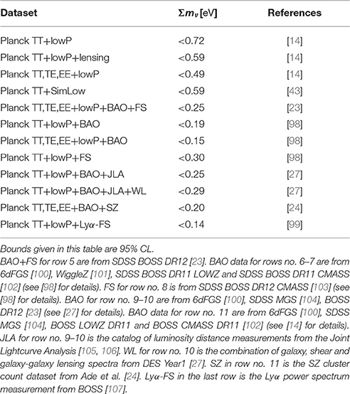
Table 1. Constraints on Σm_ν from different combination of current cosmological data.

2. Notation and Preliminaries

2.1. Basic Equations

Inferences from cosmological observations are made under the assumption that the Universe is homogeneous and isotropic, and as such it is well-described, in the context of general relativity, by a Friedmann-Lemaitre-Robertson-Walker (FLRW) metric. Small deviations from homogeneity and isotropy are modeled as perturbations over of a FLRW background.

In a FLRW Universe, expansion is described by the Friedmann equation² for the Hubble parameter H:

$\begin{array}{ll}H{(a)}^2=\frac{8\pi G}{3}\rho (a)-\frac{K}{a^2},& (1)\end{array}$

where G is the gravitational constant, K parameterizes the spatial curvature³, a is the cosmic scale factor and the ρ is the total energy density. This is given by the sum of the energy densities of the various components of the cosmic fluid.

Considering cold dark matter (c), baryons (b), photons (γ), dark energy (DE), and massive neutrinos (ν), and introducing the redshift 1 + z = a⁻¹, the Friedmann equation can be recast as:

$\begin{array}{l}H{(z)}^2=H_0^2[({\Omega }_c+{\Omega }_b){(1+z)}^3+{\Omega }_{\gamma }{(1+z)}^4+\\ +{\Omega }_{DE}{(1+z)}^{3(1+w)}+{\Omega }_k{(1+z)}^2+\frac{{\rho }_{\nu ,\text{tot}}(z)}{{\rho }_{\text{crit},0}}],& (2)\end{array}$

where we have introduced the present value of the critical density required for flat spatial geometry ${\rho }_{\text{crit},0}\equiv 3H_0^2/8\pi G$ (in general, we use a subscript 0 to denote quantities evaluated today), and the present-day density parameters Ω_i = ρ_i,0/ρ_crit,0 (since we will be always referring to the density parameters today, we omit the subscript 0 in this case). The scalings with (1 + z) come from the fact that the energy densities of non-relativistic matter and radiation scale with a⁻³ and a⁻⁴, respectively. For DE, in writing Equation (2) we have left open the possibility for an arbitrary (albeit constant) equation-of-state parameter w. In the case of neutrinos, since the parameter of their equation of state is not constant, we could not write a simple scaling with redshift, although this is possible in limiting regimes (see section 2.5). We use ρ_ν,tot to denote the total neutrino density, i.e., summed over all mass eigenstates. Finally, we have defined a “curvature density parameter” ${\Omega }_k=-K/H_0^2$. From Equation (2) evaluated at z = 0 it is clear that the density parameters, including curvature, satisfy the constrain $\sum _i{\Omega }_i=1$.

Let us also introduce some extra notation and jargon that will be useful in the following. We will use Ω_m to refer to the total density of non-relativistic matter today. Thus, this in general includes dark matter, baryons, and those neutrinos species that are heavy enough to be non-relativistic today. In such a way we have that Ω_m + Ω_DE = 1 in a flat Universe (or Ω_m + Ω_DE = 1 − Ω_k in general), since the present density of photons and other relativistic species is negligible. Since many times we will have to consider the density of matter that is non-relativistic at all the redshifts that are probed by cosmological observables, i.e., dark matter and baryons but not neutrinos, we also introduce Ω_c+b, with obvious meaning. When we consider dark energy in the form of a cosmological constant (w = −1) we use Ω_Λ in place of Ω_DE to make this fact clear. Finally, we also use the physical density parameters ${\omega }_i\equiv {\Omega }_i{h}^2$, with h being the present value of the Hubble parameter in units of 100 km s⁻¹ Mpc⁻¹.

As we shall discuss in more detail in the following, cosmological observables often carry the imprint of particular length scales, related to specific physical effects. For this reason we recall some definitions that will be useful in the following. The causal horizon r_h at time t is defined as the distance traveled by a photon from the Big Bang (t = 0) until time t. This is given by:

$\begin{array}{ll}{r}_h(t)={\displaystyle {{\displaystyle \int }}_0^t}\frac{d{t}^{\prime }}{a(t^{\prime })}={\displaystyle {{\displaystyle \int }}_{z(t)}^{\infty }}\frac{d{z}^{\prime }}{H(z^{\prime })}.& (3)\end{array}$

Note that this is actually the comoving causal horizon; in the following, unless otherwise noted, we will always use comoving distances. We also note that the comoving horizon is equal to the conformal time η(t) (defined through dt = adη and η(t = 0) = 0). In a Friedmann Universe (i.e., one composed only by matter and radiation), the physical causal horizon is proportional, by a factor of order unity, to the Hubble length $d_H(t)\equiv H{(t)}^{-1}$. For this reason, we shall sometimes indulge in the habit of calling the latter the Hubble horizon, even though this is, technically, a misnomer.

A related quantity is the sound horizon r_s(t), i.e., the distance traveled in a certain time by an acoustic wave in the baryon-photon plasma. The expression for r_s is very similar to the one for the causal horizon, just with the speed of light (equal to 1 in our units) replaced by the speed of sound c_s in the plasma:

$\begin{array}{ll}{r}_s(t)={\displaystyle {{\displaystyle \int }}_0^t}\frac{c_s(t^{\prime })}{a(t^{\prime })}d{t}^{\prime }={\displaystyle {{\displaystyle \int }}_{z(t)}^{\infty }}\frac{c_s(z^{\prime })}{H(z^{\prime })}d{z}^{\prime }.& (4)\end{array}$

The speed of sound is given by $c_s=1/\sqrt{3(1+R)}$, with R = (p_b + ρ_b)/(p_γ + ρ_γ) being the baryon-to-photon momentum density ratio. When the baryon density is negligible relative to the photons, $c_s\simeq 1/\sqrt{3}$ and $r_s\simeq r_h/\sqrt{3}=\eta /\sqrt{3}$.

Imprints on the cosmological observables of several physical processes usually depend on the value of those scales at some particular time. For example, the spacing of acoustic peaks in the CMB spectrum is reminiscent of the sound horizon at the time of hydrogen recombination; the suppression of small-scale matter fluctuations due to neutrino free-streaming is set by the causal horizon at the time neutrinos become non-relativistic; and so on. Moreover, since today we see those scales through their projection on the sky, what we observe is actually a combination of the scale itself and the distance to the object that we are observing. We find then useful also to recall some notions related to cosmological distances. The comoving distance χ between us and an object at redshift z is

$\begin{array}{ll}\chi (z)={\displaystyle {{\displaystyle \int }}_0^z}\frac{d{z}^{\prime }}{H(z^{\prime })},& (5)\end{array}$

and this is also equal to η₀ − η(z). The comoving angular diameter distance d_A(z) is given by

$\begin{array}{ll}{d}_A(z)=\frac{sin(\sqrt{K}\chi )}{\sqrt{K}},& (6)\end{array}$

so that

$\begin{array}{ll}{d}_A(z)=\chi (z)={\displaystyle {{\displaystyle \int }}_0^z}\frac{d{z}^{\prime }}{H(z^{\prime })}\text{ for}{\Omega }_k=0.& (7)\end{array}$

The angular size θ of an object is related to its comoving linear size λ through θ = λ/d_A(z). This justifies the definition of an object of known linear size as a standard ruler for cosmology. In fact, knowing λ, we can use a measure of θ to get d_A and make inferences on the cosmological parameters that determine its value through the integral in Equation (6).

Another measure of distance is given by the luminosity distance d_L(z), that relates the observed flux F to the intrinsic luminosity L of an object at redshift z:

$\begin{array}{ll}{d}_L(z)\equiv \sqrt{\frac{L}{4\pi F}}=(1+z)d_A(z).& (8)\end{array}$

Similarly to what happened for the angular diameter distance, this allows to use standard candles—objects of known intrinsic luminosity—as a mean to infer the values of cosmological parameters, after their flux has been measured.

2.2. Neutrino Mass Parameters

According to the standard theory of neutrino oscillations, the observed neutrino flavors ν_α (α = e, μ, τ) are quantum superpositions of three mass eigenstates ν_i (i = 1, 2, 3):

$\begin{array}{ll}|{\nu }_{\alpha }\rangle ={\displaystyle \sum _i{U}_{\alpha i}^{*}}|{\nu }_i\rangle ,& (9)\end{array}$

where U is the Pontecorvo-Maki-Nakagawa-Sasaka (PMNS) mixing matrix. The PMNS matrix is parameterized by three mixing angles θ₁₂, θ₁₃, θ₂₃, and three CP-violating phases: one Dirac, δ, and two Majorana phases, α₂₁ and α₃₁. The Majorana phases are non-zero only if neutrinos are Majorana particles. They do not affect oscillation phenomena, but enter lepton number-violating processes like 0ν2β decay. The actual form of the PMNS matrix is:

$\begin{array}{l}U=\left[\begin{array}{ccc}{c}_{12}{c}_{13}& s_{12}{c}_{13}& s_{13}{e}^{-i\delta }\\ -s_{12}{c}_{23}-c_{12}{s}_{23}{s}_{13}{e}^{i\delta }& c_{12}{c}_{23}-s_{12}{s}_{23}{s}_{13}{e}^{i\delta }& s_{23}{c}_{13}\\ s_{12}{s}_{23}-c_{12}{c}_{23}{s}_{13}{e}^{i\delta }& -c_{12}{s}_{23}-s_{12}{c}_{23}{s}_{13}{e}^{i\delta }& c_{23}{c}_{13}\end{array}\right]\\ \times \text{ diag }(1,e^{i{\alpha }_{21}/2},e^{i{\alpha }_{31}/2}),& (10)\end{array}$

where c_ij ≡ cos θ_ij and s_ij ≡ sin θ_ij.

In addition to the elements of the mixing matrix, the other parameters of the neutrino sector are the mass eigenvalues m_i (i = 1, 2, 3). Oscillation experiments have measured with unprecedented accuracy the three mixing angles and the two mass squared differences relevant for the solar and atmospheric transitions, namely the solar splitting $\Delta m_{\text{sol}}^2=\Delta m_{21}^2\equiv m_2^2-m_1^2\simeq 7.6\times 10^{-5}\text{e}{\text{V}}^2$, and the atmospheric splitting $\Delta m_{\text{atm}}^2=|\Delta m_{31}^2|\equiv |m_3^2-m_1^2|\simeq 2.5\times 10^{-3}\text{e}{\text{V}}^2$ (see e.g., [39–41] for a global fit of the neutrino mixing parameters and mass splittings). We know, because of matter effects in the Sun, that, of the two eigenstates involved, the one with the smaller mass has the largest electron fraction. By convention, we identify this with eigenstate “1,” so that the solar splitting is positive. On the other hand, we do not know the sign of the atmospheric mass splitting, so this leaves open two possibilities: the normal hierarchy (NH), where $\Delta m_{31}^2>0$ and m₁ < m₂ < m₃, or the inverted hierarchy, where $\Delta m_{31}^2<0$ and m₃ < m₁ < m₂.

Oscillation experiments are unfortunately insensitive to the absolute scale of neutrino masses. In this review, we will mainly focus on cosmological observations as a probe of the absolute neutrino mass scale. To a very good approximation, cosmological observables are mainly sensitive to the sum of neutrino masses Σm_ν, defined simply as

$\begin{array}{ll}\Sigma m_{\nu }\equiv {\displaystyle \sum _i}{m}_i.& (11)\end{array}$

Absolute neutrino masses can also be probed by laboratory experiments. These will be reviewed in more detail in section 9, where their complementarity with cosmology will be also discussed. For the moment, we just recall the definition of the mass parameters probed by laboratory experiments. The effective (electron) neutrino mass m_β

$\begin{array}{ll}{m}_{\beta }={\left({\displaystyle \sum _i}|U_{ei}{|}^2{m}_i^2\right)}^{1/2},& (12)\end{array}$

can be constrained by kinematic measurements like those exploiting the β decay of nuclei. The effective Majorana mass of the electron neutrino m_ββ:

$\begin{array}{ll}{m}_{\beta \beta }=\left|{\displaystyle \sum _i}{U}_{ei}^2{m}_i\right|,& (13)\end{array}$

can instead be probed by searching for 0ν2β decay.

2.3. The Standard Cosmological Model

Our best description of the Universe is currently provided by the spatially flat ΛCDM model with adiabatic, nearly scale-invariant initial conditions for scalar perturbations. With the exception of some mild (at the ~2σ level) discrepancies that will be discussed in the part devoted to observational limits, all the available data can be fit in this model, that in its simplest (“base”) version is described by just six parameters. In the base ΛCDM model, the Universe is spatially flat (Ω_k = 0), and the matter and radiation content is provided by cold dark matter, baryons, photons, and neutrinos, while dark energy is in the form of a cosmological constant (w = −1). The energy density of photons is fixed by measurements of the CMB temperature, while neutrinos are assumed to be very light, usually fixing the sum of the masses to Σm_ν = 0.06 eV, the minimum value allowed by oscillation experiments. In this way, the energy density of neutrinos is also fixed at all stages of the cosmological evolution (see section 2.5). From Equation (2), and taking into account the flatness constraint, it is clear then that the background evolution in such a model is described by three parameters, for example⁴ h, ω_c, and ω_b, with Ω_Λ given by 1 − Ω_m. The initial scalar fluctuations are adiabatic and have a power-law, nearly scale invariant, spectrum, that is thus parameterized by two parameters, an amplitude A_s and a logarithimc slope n_s − 1 (with n_s = 1 thus corresponding to scale invariance). Finally, the optical depth to reionization τ parameterizes the ionization history of the Universe.

This simple, yet very successful, model can be extended in several ways. The extension that we will be most interested in, given the topic of this review, is a one-parameter extension in which the sum of neutrino masses is considered as a free parameter. We call this seven-parameter model ΛCDM + Σm_ν. This is also in some sense the best-motivated extension of ΛCDM, as we actually know from oscillation experiments that neutrinos have a mass, and from β-decay experiments that this can be as large as 2 eV. In addition to this minimal extension, we will also discuss how relaxing some of the assumptions of the ΛCDM model affects estimates of the neutrino mass. Among the possibilities that we will consider, there are those of varying the curvature (Ω_k), the equation-of-state parameter of dark energy (w), or the density of radiation in the early Universe (N_eff, defined in section 2.5).

There are many relevant extensions to the ΛCDM model that however we will not consider here (or just mention briefly). The most important one concerns the possibility of non-vanishing tensor perturbations, i.e., primordial gravitational waves, that, if detected, would provide a smoking gun for inflation. This scenario is parameterized through an additional parameter, the tensor-to-scalar ratio r. In the following, we will always assume r = 0. In any case, this assumption will not affect the estimates reported here, as the effect of finite neutrino mass and of tensor modes on the cosmological observables are quite distinct. Similarly, we will not consider the possibility of non-adiabatic initial perturbations, nor of more complicated initial spectra for the scalar perturbations, including those with a possible running of the scalar spectral index, although we report a compilation of relevant references in section 7 for the reader's convenience.

2.4. Short Thermal History

Given that cosmological observables carry the imprint of different epochs in the history of the Universe, we find it useful to shortly recall some relevant events taking place during the expansion history, and their relation to the cosmological parameters. For our purposes, it is enough to start when the temperature of the Universe was T ~ 1 MeV, i.e., around the time of Big Bang Nucleosynthesis (BBN) and neutrino decoupling. At these early times (z ~ 10¹⁰), since matter and radiation densities scale as (1 + z)³ and (1 + z)⁴, respectively, the Universe is radiation-dominated.

• At T ~ 1 MeV (z ~ 10¹⁰), the active neutrinos decouple from the rest of the cosmological plasma. Before this time, neutrinos were kept in equilibrium by weak interactions with electrons and positrons, that were in turn coupled electromagnetically to the photon bath. After this time, the neutrino mean free path becomes much larger the the Hubble length, so they essentially move along geodesics, i.e., they free-stream. Shortly after neutrino decouple, electrons and positrons in the Universe annihilate, heating the photon-electron-baryon plasma, and, to a much lesser extent, the neutrino themselves (in section 2.5 we shall discuss in more detail the neutrino thermal history). After this time, the Universe can essentially be thought as composed of photons, electrons, protons and neutrons (either free, or, after BBN, bound together into the light nuclei), neutrinos, dark matter, and dark energy.

• Soon after, at T ~ 0.1 MeV, primordial nucleosynthesis starts, and nuclear reactions bind nucleons into light nuclei. After this time, nearly all of the baryons in the Universe are in the form of ¹H and ⁴He nuclei, with small traces of ²H and ⁷Li. The yields of light elements strongly depend on the density of baryons, on the density and energy spectrum of electron neutrinos and antineutrinos (as those set the equilibrium of the nuclear reactions) and on the total radiation density (as this sets the expansion rate at the time of nucleosynthesis).

• As said above, at early times (high z) the Universe is radiation-dominated, given that the radiation-to-matter density ratio like (1 + z). However, the radiation density decreases faster than that of matter, and, at some redshift z_eq, the matter and radiation contents of the Universe will be equal: ρ_m(z_eq) = ρ_r(z_eq). This is called the epoch of matter-radiation equality, that marks the beginning of the matter-dominated era in the history of the Universe. From the scaling of the two densities, it is easy to see that 1 + z_eq = Ω_m/(Ω_γ + Ω_ν) in a Universe with massless neutrinos (so that their density always scale as (1 + z)⁴; see section 2.5 for further discussion on this point). Given the current estimates of cosmological parameters, z_eq ≃ 3, 400 [14].

• At T ≃ 0.3 eV, electrons and nuclei combine to form neutral hydrogen and helium, that are transparent to radiation. This recombination epoch thus roughly corresponds to the time of decoupling of radiation from matter. This is the time at which the CMB radiation is emitted. After decoupling, the CMB photons undergo last interactions with residual free electrons. Finally, the CMB photons emerge from this last scattering surface and free-stream until the present time (with some caveats, see below). Most of the features that we observe in the CMB anisotropy pattern are created at this time. Given the current estimates of cosmological parameters, z_rec ≃ 1, 090 [14]. Note that in fact the temperature at recombination is basically fixed by thermodynamics, so once the present CMB temperature is determined through observations, z_rec = T(z = z_rec)/T(z = 0) depends very weakly on the other cosmological parameters.

• Even if photons decoupled from matter shortly after recombination, the large photon-to-baryon ratio keeps baryons coupled to the photon bath for some time after that. The drag epoch z_drag is the time at which baryons stop feeling the photon drag. A good fit to numerical results in a CDM cosmology is given by Eisenstein and Hu [42]

$\begin{array}{l}{z}_{\text{drag}}=1,291\frac{{({\omega }_c+{\omega }_b)}^{0.251}}{1+0.659{({\omega }_c+{\omega }_b)}^{0.828}}\left[1+b_1{({\omega }_c+{\omega }_b)}^{b_2}\right],\\ b_1=0.313{({\omega }_c+{\omega }_b)}^{-0.419}\left[1+0.607{({\omega }_c+{\omega }_b)}^{0.674}\right],\\ b_2=0.238{({\omega }_c+{\omega }_b)}^{0.223}& (14)\end{array}$

Given the current estimates of cosmological parameters, z_drag ≃ 1,060 [14].

• For a long time after recombination, the Universe stays transparent to radiation. These are the so-called “dark ages.” However, in the late history of the Universe, the neutral hydrogen gets ionized again due to UV emission of the first stars, that puts an end to the dark ages. This is called the reionization epoch. After reionization, the CMB photons are scattered again by the free electrons. Given the current estimates of cosmological parameters, z_re ≃ 8 [43].

• At some point during the recent history of the Universe, that we denote with z_Λ, the energy content of the Universe starts to be dominated by the dark energy component. The end of matter domination, and the beginning of this DE domination is set by ρ_DE(z_Λ) = ρ_m(z_Λ). For a cosmological constant (w = −1), $1+z_{\Lambda }={({\Omega }_{\Lambda }/{\Omega }_m)}^{1/3}$. Given the current estimates of cosmological parameters, z_Λ ≃ 0.3 [14]. Around this time, the cosmological expansion becomes accelerated.

2.5. Evolution of Cosmic Neutrinos

In this section, we discuss the thermal history of cosmic neutrinos.

As anticipated above, in the early Universe neutrinos are kept in equilibrium with the cosmological plasma by weak interactions. The two competing factors that determine if equilibrium holds are the expansion rate, given by the Hubble parameter H(z), and the interaction rate Γ(z) = n〈σv〉, where n is the number density of particles, σ is the interaction cross section, and v is the velocity of particles (brackets indicate a thermal average). In fact, neutrino interactions become too weak to keep them in equilibrium once Γ < H. The left-hand side of this inequality is set by the standard model of particle physics, as the interaction rate at a given temperature only depends on the cross-section for weak interactions, and thus, ultimately, on the value of the Fermi constant (${\sigma }_w~G_F^2{T}^2$). The right-hand side is instead set through Equation (2) by the total radiation density (the only relevant component at such early times): $H^2=(8\pi G/3)({\rho }_{\gamma }+{\rho }_{\nu })$. In the framework of the minimal ΛCDM model, once the present CMB temperature is measured, the radiation density at any given temperature is fixed. Thus the temperature of neutrino decoupling, defined through Γ(T_ν,dec) = H(T_ν,dec) does not depend on any free parameter in the theory. A quite straightforward calculation shows that T_ν,dec ≃ 1 MeV [44].

While they are in equilibrium, the phase-space distribution f(p) of neutrinos is a Fermi-Dirac distribution⁵:

$\begin{array}{ll}f(p,t)=\frac{1}{e^{p/T_{\nu }(t)}+1},& (15)\end{array}$

where it has been taken into account that at T ≳ 1 MeV, the active neutrinos are certainly ultrarelativistic (i.e., T_ν ≫ m_ν) and thus E(p) ≃ p. The distribution does not depend on the spatial coordinate $\overrightarrow{x}$, nor on the direction of momentum $\widehat{p}$, due to the homogeneity and isotropy of the Universe. Before decoupling, the neutrino temperature T_ν is the common temperature of all the species in the cosmological plasma, that we denote generically with T, so that T_ν = T. We recall that the temperature of the plasma evolves according to $g_{*s}^{1/3}aT=\text{const}.$, where g_∗s counts the effective number of relativistic degrees of freedom that are relevant for entropy [44].

Since decoupling happens while neutrinos are ultrarelativistic, it can be shown that, as a consequence of the Liouville theorem, the shape of the distribution function is preserved by the expansion. In other words, the distribution function still has the form Equation (15), with an effective temperature T_ν(z) (that for the sake of simplicity we will continue to refer to as the neutrino temperature) that scales like a⁻¹ (i.e., aT = const). We stress that this means that, when computing integrals over the distribution function, one still neglects the mass term in the exponential of the Fermi-Dirac function, even at times when neutrinos are actually non-relativistic.

Shortly after neutrino decouple, electrons and positrons annihilate and transfer their entropy to the rest of the plasma, but not to neutrinos. In other words, while the neutrino temperature scales like a⁻¹, the photon temperature scales like $a^{-1}{g}_{*s}^{-1/3}$, and thus decreases slightly more slowly during e⁺e⁻ annihilation, when g_∗s is decreasing. In fact, applying entropy conservation one finds that the ratio between the neutrino and photon temperatures after electron-positron annihilation is $T_{\nu }/T={(4/11)}^{1/3}$. The photon temperature has been precisely determined by measuring the frequency spectrum of the CMB radiation: T₀ = (2.725 ± 0.002) K [45, 46], so that the present temperature of relic neutrinos should be T_ν,0 ≃ 1.95 K ≃ 1.68 × 10⁻⁴ eV.

The number density n_ν of a single neutrino species (including both neutrinos and their antiparticles) is thus given by:

$\begin{array}{ll}{n}_{\nu }(T_{\nu })=\frac{g}{{(2\pi )}^3}{\displaystyle \int }\frac{d^{3}p}{e^{p/T_{\nu }}+1}=\frac{3\zeta (3)}{4{\pi }^2}{T}_{\nu }^3,& (16)\end{array}$

where ζ(3) is the Riemann zeta function of 3, and in the last equality we have taken into account that g = 2 for neutrinos. This corresponds to a present-day density of roughly 113 particles/cm³.

The energy density of a single neutrino species is instead

$\begin{array}{ll}{\rho }_{\nu }(T_{\nu })=\frac{g}{{(2\pi )}^3}{\displaystyle \int }\frac{\sqrt{p^2+m^2}}{e^{p/T_{\nu }}+1}{d}^{3}p.& (17)\end{array}$

This is the quantity that appears, among other things, in the right-hand side of the Friedmann equation (summed over all mass eigenstates). In the ultrarelativistic (T_ν ≫ m) and non-relativistic (T_ν ≪ m) limits, the energy density takes simple analytic forms:

$\begin{array}{ll}{\rho }_{\nu }(T_{\nu })=\{\begin{array}{ll}\frac{7{\pi }^2}{120}{T}_{\nu }^4\hfill & (\text{UR})\hfill \\ m_{\nu }{n}_{\nu }\hfill & (\text{NR})\hfill \end{array}& (18)\end{array}$

These scalings are consistent with the fact that one expects neutrinos to behave as pressureless matter, ${\rho }_{\nu }\propto {(1+z)}^3$, in the non-relativistic regime, and as radiation, ${\rho }_{\nu }\propto {(1+z)}^4$, in the ultrarelativistic regime.

Given that the present-day neutrino temperature is fixed by measurements of the CMB temperature and by considerations of entropy conservation, it is clear from the above formulas how the present energy density of neutrinos depends only on one free parameter, namely the sum of neutrino masses Σm_ν defined in Equation (11). Introducing the total density parameter of massive neutrinos ${\Omega }_{\nu }\equiv \sum _i{\rho }_{{\nu }_i,0}/{\rho }_{\text{crit},0}$, one easily finds from Equation (16):

$\begin{array}{ll}{\Omega }_{\nu }{h}^2=\frac{\Sigma m_{\nu }}{93.14\text{ eV}}.& (19)\end{array}$

where we have already included the effects of non-instantaneous neutrino decoupling, see below. In the instantaneous decoupling approximation, the quantity at denominator would be 94.2 eV.

On the other hand, the neutrino energy density in the early Universe only depends on the neutrino temperature, and thus it is completely fixed in the framework of the ΛCDM model. Using the fact that for photons ${\rho }_{\gamma }=({\pi }^2/15)T^4$, together with the relationship between the photon and neutrino temperatures, one can write for the total density in relativistic species in the early Universe, after e⁺e⁻ annihilation:

$\begin{array}{ll}{\rho }_{\gamma +\nu }={\rho }_{\gamma }\left[1+\frac{7}{8}{\left(\frac{4}{11}\right)}^{4/3}{N}_{\nu }\right],& (20)\end{array}$

where N_ν is the number of neutrino families. In the framework of the standard model of particle physics, considering the active neutrinos, one has N_ν = 3. However, the above formula slightly underestimates the total density at early times; the main reason is that neutrinos are still weakly coupled to the plasma when e⁺e⁻ annihilation occurs, so that they share a small part of the entropy transfer. Moreover, finite temperature QED radiative corrections and flavor oscillations also play a role. This introduces non-thermal distortions at the subpercent level in the neutrino energy spectrum; the integrated effect is that at early times the combined energy densities of the three neutrino species are not exactly equal to 3ρ_ν, with ρ_ν given by the upper row of Equation (18), but instead are given by (3.046ρ_ν) [12, 47]. A recent improved calculation, including the full collision integrals for both the diagonal and off-diagonal elements of the neutrino density matrix, has refined this value to (3.045ρ_ν) [48]. It is then customary to introduce an effective number of neutrino families N_eff and rewrite the energy density at early times as:

$\begin{array}{ll}{\rho }_{\gamma +\nu }={\rho }_{\gamma }\left[1+\frac{7}{8}{\left(\frac{4}{11}\right)}^{4/3}{N}_{\text{eff}}\right].& (21)\end{array}$

In this review, we will consider N_eff = 3.046 as the “standard” value of this parameter in the ΛCDM model, and not the more precise value found in de Salas and Pastor [48], since most of the literature still makes use of the former value. This does not make any difference, however, from the practical point of view, given the sensitivity of present and next-generation instruments.

It is also customary to consider extensions of the minimal ΛCDM model in which one allows for the presence of additional light species in the early Universe (“dark radiation”). In this kind of extension, the total radiation density of the Universe is still given by the right-hand side of Equation (21), where now however N_eff has become a free parameter. In other words, Equation (21) becomes a definition for N_eff, that is, just a way to express the total energy density in radiation. The effect on the expansion history of this additional radiation component can be taken into account by the substitution

$\begin{array}{ll}{\Omega }_{\gamma }\to {\Omega }_{\gamma }\left[1+\frac{7}{8}{\left(\frac{4}{11}\right)}^{4/3}\Delta N_{\text{eff}}\right]& (22)\end{array}$

in the rhs of the Hubble equation (2), with ΔN_eff ≡ N_eff − 3.046. Note that this substitution fully captures the effect of the additional species only if this is exactly massless, and not just very light (as in the case of a light massive sterile neutrino, for example—see section 10).

It is often useful, to understand some of the effects that we will discuss in the following, to have a feeling for the time at which neutrinos of a given mass become non-relativistic, or, thinking the other way around, for the mass of a neutrino that becomes non-relativistic at a given redshift. The average momentum of neutrinos at a temperature T_ν is 〈p〉 = 3.15T_ν. We take as the moment of transition from the relativistic to the non-relativistic regime the time when 〈p〉 = m_ν. Then, using the fact that $T_{\nu }(z)={(4/11)}^{1/3}{T}_0(1+z)=1.68\times 10^{-4}(1+z)\text{ eV}$, one has

$\begin{array}{ll}1+z_{\text{nr}}\simeq 1,900\left(\frac{m_{\nu }}{\text{eV}}\right).& (23)\end{array}$

This relation can be used to show e.g., that neutrinos with mass m_ν ≲ 0.6 eV turn non-relativistic around or after recombination. In the following, when discussing the effect of neutrino masses on the CMB anisotropies, we will assume that this is the case. Note however that the actual statistical analyses from which bounds on neutrino masses are derived do not make such an assumption. We also note that, given the current measurements of the neutrino mass differences, only the lightest mass eigenstate can still be relativistic today. Thus at least two out of the three active neutrinos become non-relativistic before the present time.

We conclude this section with a clarification on the role of neutrinos in determining the redshift of matter-radiation equality. Given the present bounds on neutrino masses, we know that equality likely takes place when neutrino are relativistic. In fact, observations of the CMB anisotropies constrain z_eq ≃ 3,400, so that neutrinos with mass m_ν ≃ 1.8 eV, just below the current bound from tritium beta-decay, turn non-relativistic at equality. Thus, for masses sufficiently below the tritium bound, the total density of matter at those times is proportional to Ω_c+b. The radiation density is instead provided by photons and by the relativistic neutrinos (and as such does not depend on the neutrino mass), plus any other light species present in the early Universe. So the redshift of equivalence is given by

$\begin{array}{ll}1+z_{\text{eq}}=\frac{{\Omega }_c+{\Omega }_b}{{\Omega }_{\gamma }\left[1+\frac{7}{8}{\left(\frac{4}{11}\right)}^{4/3}{N}_{\text{eff}}\right]}=\frac{{\omega }_c+{\omega }_b}{{\omega }_{\gamma }\left[1+\frac{7}{8}{\left(\frac{4}{11}\right)}^{4/3}{N}_{\text{eff}}\right]},& (24)\end{array}$

where the last equality makes it clear that, in the framework of the minimal ΛCDM model, the redshift of equivalence only depends on the quantity ω_c+ω_b, since N_eff is fixed and ω_γ is determined through observations (it is basically the CMB energy density).

3. Cosmological Effects of Neutrino Masses

The impact of neutrino masses—and in general of neutrino properties—on the cosmological evolution can be divided in two broad categories: background effects, and perturbation effects. The former class refers to modifications in the expansion history, i.e., in changes to the evolution of the FLRW background. The latter class refers instead to modifications in the evolution of perturbations in the gravitational potentials and in the different components of the cosmological fluid. We shall now briefly review both classes; we refer the reader who is interested in a more detailed analysis to the excellent review by Lesgourgues and Pastor [13].

To start, we shall consider a spatially flat Universe, i.e., Ω_k = 0, in which dark energy is in the form of a cosmological constant (w = −1) and there are no extra radiation components (N_eff = 3.046). Let us also consider a particular realization of this scenario, that we refer to as our reference model, in which the sum of neutrino masses is very small; for definiteness, we can think that Σm_ν is equal to the minimum value allowed by oscillation measurements, Σm_ν = 0.06 eV (see section 8 for further details). When needed, we will take the other parameters as fixed to their ΛCDM best-fit values from Planck 2015 [14]. Our aim is to understand what happens when we change the value of Σm_ν. Increasing the sum of neutrino masses Σm_ν will increase ${\omega }_{\nu }={\Omega }_{\nu }{h}^2$ according to Equation (19). Remember that the sum of the density parameters $\sum _i{\Omega }_i=1$; this constraint can be recast in the form:

$\begin{array}{ll}{\omega }_c+{\omega }_b+{\omega }_{\Lambda }+{\omega }_{\gamma }+{\omega }_{\nu }+{\omega }_k=h^2.& (25)\end{array}$

Since ω_γ is constrained by observations, and ω_k is zero by assumption, we have four degrees of freedom that we can use to compensate for the change in ω_ν, namely: increase h, or decrease any of ω_c, ω_b, or ω_Λ. For the moment, for simplicity, we will not distinguish between baryons and cold dark matter, pretending that as non-relativistic components they have the same effect on cosmological observables. This is of course not the case, but we will come back to this later. Then we are left with three independent degrees of freedom that we can use to compensate for the change in ω_ν: h, ω_b+c, and ω_Λ. We prefer to use Ω_Λ in place of ω_Λ, so that in the end our parameter basis for this discussion will be {h, ω_c+b, Ω_Λ}.

The first option, increasing the present value of the Hubble constant while keeping Ω_Λ and ω_b+c constant has the effect of making the Hubble parameter at any given redshift after neutrinos become non-relativistic larger with respect to the reference model. This can be understood by looking at Equation (2), that we rewrite here in this particular case

$\begin{array}{l}H{\left(z\right)}^2=H_0^2[({\Omega }_c+{\Omega }_b){(1+z)}^3+{\Omega }_{\gamma }{(1+z)}^4\hfill \\ +{\Omega }_{\Lambda }+\frac{{\rho }_{\nu ,\text{tot}}(z)}{{\rho }_{\text{crit},0}}].\hfill & (26)\end{array}$

With respect to the reference model, the first two terms in the RHS are unchanged, while the third increases because Ω_Λ is fixed but h is larger. The last term does not depend on h (because the factor $H_0^2$ in front of the square brackets cancel the one in the critical density) but yet increases because ρ_ν = Σm_νn_ν is larger as long as neutrinos are in the non-relativistic regime. On the other hand, before neutrino become non-relativistic, ρ_ν is the same in the two models, and the change in the ${\Omega }_{\Lambda }{h}^2$ term is irrelevant, because the DE density is only important at very low redshifts. So we can conclude that at z ≫ z_nr, the two models share the same expansion history, while for z ≲ z_nr the model with “large” neutrino mass is always expanding faster (larger H), or equivalently, is always younger, at those redshifts. In terms of the length scales and of the distance measures introduced in section 2.1, it is easily seen that the causal and sound horizons at both equality and recombination (as well as at the drag epoch) are unchanged, because the expansion history between z = ∞ and z ≃ z_nr is unchanged. On the other hand, distances between us and objects at any redshift—for example, the angular diameter distance to recombination—are always smaller than in the reference model, because H is always larger between z ≃ z_nr and z = 0. H increases with the extra neutrino density, so this effect increases with larger neutrino masses (and moreover, z_nr also gets larger for larger masses). Given this, we expect for example the angle subtended by the sound horizon at recombination, θ_s = r_s(z_rec)/d_A(z_rec) to become larger when we increase Σm_ν. We conclude this part of the discussion that in this case the redshift of equality z_eq does not change, since ω_b+c is being kept constant, and neutrinos contribute to the radiation density at early times (see discussion at the end of the previous section).

If we instead choose to pursue the second option, i.e., we keep h and Ω_Λ constant while lowering ω_c+b, we are again changing the expansion history, but this time on a different range of redshifts. In fact, when neutrinos are non-relativistic, the RHS of Equation (26) is unchanged, because the changes in the present-day densities of neutrinos and non-relativistic matter perfectly compensate; this continues to hold as long as both densities scale as (1 + z)³, i.e., roughly for z < z_nr. On the other hand, at z > z_nr the neutrino density is the same as in the reference model, while the matter density is smaller, so H(z) is smaller as well. Finally, when the Universe is radiation dominated, the two models share again the same expansion history. Then in this scenario we change the expansion history, decreasing H, for z_nr ≲ z ≲ z_eq. The sound horizon at recombination increases, and so does the angular diameter distance, so one cannot immediately guess how their ratio varies. However, a direct numerical calculation shows that, starting from the Planck best-fit model, the net effect is to increase θ_s, meaning that the sound horizon will subtend a larger angular scale on the sky when Σm_ν increases. For what concerns instead the redshift of matter-radiation equality, it is immediate to see that it decreases proportionally to ω_c+b, i.e., equality happens later in the model with larger Σm_ν.

Finally, when Ω_Λ is decreased, the main effect is to delay the onset of acceleration and make the matter-dominated era last longer. This has some effect on the evolution of perturbations, as we shall see in the following. For what concerns the expansion history, since the model under consideration and the reference model only differ in the neutrino mass and in the DE density, they are identical when neutrinos are relativistic and DE is negligible, i.e., at z > z_nr. For z < z_nr, instead, starting as usual from Equation (26) one finds, with some little algebra, that H(z) is always larger in the model with smaller Ω_Λ and larger Σm_ν. As in the previous case, both r_s and d_A at recombination vary in the same direction (decreasing in this case); the net effect is again that θ_s becomes larger with Σm_ν. Also, since the matter density at early times is not changing in this case, the redshift of equivalence is the same in the two models.

We now comment briefly about ω_b. One could choose to modify ω_b in place of ω_c in order to compensate for the change in ω_ν. From the point of view of the background expansion, both choices are equivalent, since the baryon and cold dark matter density only enter through their sum ω_b+c in the RHS of Equation (26). However, changing the baryon density also produces some peculiar effects, mainly related to the fact that (i) it determines the BBN yields, and (ii) it affects the evolution of photon perturbations prior to recombination. Thus, the density of baryons is quite well constrained by the observed abundances of light elements and by the relative ratio between the heights of odd and even peaks in the CMB, (see section 4.1) and there is little room for changing it without spoiling the agreement with observations.

Let us now turn to discuss the effects on the evolution of perturbations. Given that we have observational access to the fluctuations in the radiation and matter fields, it is useful to discuss separately these two components. The photon perturbations are sensitive to time variations in the gravitational potentials along the line of sight from us up to the last-scattering surface; this is the so-called integrated Sachs-Wolfe (ISW) effect. The gravitational potentials are constant in a purely matter-dominated Universe, so that the observed ISW gets an early contribution right after recombination, when the radiation component is not yet negligible, and a late contribution, when the dark energy density begins to be important. Coming back to our previous discussion, it is clear to see how delaying the time of equality will increase the amount of early ISW, while anticipating dark energy domination will increase the late ISW, and viceversa. For what concerns matter inhomogeneities, a first effect is again related to the time of matter-radiation equality. Changing z_eq affects the growth of perturbations, since most of the growth happens during the matter dominated era. Apart from that, a very peculiar effect is related to the clustering properties of neutrinos. In fact, while neutrinos are relativistic, they tend to free stream out of overdense regions, damping out all perturbations below the horizon scale. The net effect is that neutrino clustering is suppressed below a certain critical scale, the free-streaming scale, that corresponds to the size of the horizon at the time of the nonrelativistic transition. If the transition happens during matter domination, this is given by:

$\begin{array}{ll}{k}_{\text{fs}}\simeq 0.018{\Omega }_m^{1/2}{\left(\frac{m_{\nu }}{1\text{eV}}\right)}^{1/2}h\text{Mp}{\text{c}}^{-1}.& (27)\end{array}$

On the contrary, above the free-streaming scale neutrinos cluster as dark matter and baryons do. Thus, increasing the neutrino mass and consequently the neutrino energy density will suppress small-scale matter fluctuations relative to the large scales. It will also make small-scale perturbations in the other components grow slower, since neutrino do not source the gravitational potentials at those scales. It should also be noted that the free-streaming scale depends itself on the neutrino mass—specifically, heavier neutrinos will become non-relativistic earlier and the free-streaming scale will be correspondingly smaller. Moreover, there is actually a free-streaming scale for each neutrino species, each depending on the individual neutrino mass. In principle one could think to go beyond observing just the small-scale suppression and try to access instead the scales around the non-relativistic transition(s), in order to get more leverage on the mass and perhaps also on the mass splitting. We shall see however in the following that this is not the case.

The suppression of matter fluctuations due to neutrino free-streaming also affects the path of photons coming from distant sources, since those photons will be deflected by the gravitational potentials along the line of sight, resulting in a gravitational lensing effect. This is relevant for the CMB, as it modifies the anisotropy pattern by mixing photons that come from different directions. Another application of this effect, of particular importance for estimates of neutrino masses, is to use the distortions of the shape of distant galaxies due to lensing, to reconstruct the intervening matter distribution.

4. Cosmological Observables

In this section we review the various cosmological observables, and explain how the effects described in the previous section propagate to the observables.

4.1. CMB Anisotropies

The CMB consists of polarized photons that, for the most part, have been free-streaming from the time of recombination to the present time. The pattern of anisotropies in both temperature (i.e., intensity) and polarization thus encodes a wealth of information about the early Universe, down to z = z_rec ≃ 1, 100. Moreover, given that the propagation of photons from decoupling to the present time is also affected by the cosmic environment, the CMB also has some sensitivity to physics at z < z_rec. Two relevant examples for the topic under consideration are the CMB sensitivity to the redshift of reionization (because the CMB photons are re-scattered by the new population of free electrons) and to the integrated matter distribution along the line of sight (because clustering at low redshifts modifies the geodesics with respect to an unperturbed FLRW Universe, resulting in a gravitational lensing of the CMB, see next section). However, the CMB sensitivity to these processes is limited due to the fact that these are integrated effects.

The information in the CMB anisotropies is encoded in the power spectrum coefficients $C_{\ell }^{TT}$, i.e., the coefficients of the expansion in Legendre polynomials of the two-point correlation function. In the case of the temperature angular fluctuations $\Delta T(\widehat{n})/\overline{T}$:

$\begin{array}{ll}\langle \frac{\Delta T(\widehat{n})}{\overline{T}}\frac{\Delta T({\widehat{n}}^{\prime })}{\overline{T}}\rangle ={\displaystyle \sum _{\ell =0}^{\infty }}\frac{2\ell +1}{4\pi }{C}_{\ell }^{TT}{P}_{\ell }(\widehat{n}·{\widehat{n}}^{\prime }).& (28)\end{array}$

For Gaussian fluctuations, all the information contained in the anisotropies can be compressed without loss in the two-point function, or equivalently in its harmonic counterpart, the power spectrum. A similar expression holds for the polarization field and for its cross-correlation with temperature. In detail, the polarization field can be decomposed into two independent components, known as E− (parity-even and curl-free) and B− (parity-odd and divergence-free) modes. Given that, it is clear that we can build a total of six spectra $C_{\ell }^{XY}$ with X, Y = T, E, B; however, if parity is not violated in the early Universe, the TB and EB correlations are bound to vanish. Let us also recall that, in linear perturbation theory, B modes are not sourced by scalar fluctuations. Thus, in the framework of the standard inflationary paradigm, primordial B modes can only be sourced in the presence of tensor modes, i.e., gravitational waves.

The shape of the observed power spectra is the result of the processes taking place in the primordial plasma around the time of recombination. In brief, in the early Universe, standing, temporally coherent acoustic waves set in the coupled baryon-photon fluid, as a result of the opposite action of gravity and radiation pressure [49]. Once the photons decouple after hydrogen recombination, the waves are “frozen” and thus we observe a series of peaks and throughs in the temperature power spectrum, corresponding to oscillation modes that were caught at an extreme of compression or rarefaction (the peaks), or exactly in phase with the background (the throughs). The typical scale of the oscillations is set by the sound horizon at recombination r_s(z_rec), i.e., the distance traveled by an acoustic wave from some very early time until recombination, see Equation (4). The position of the first peak in the CMB spectrum is set by the value of this quantity and corresponds to a perturbation wavenumber that had exactly the time to fully compress once. The second peak corresponds to the mode with half the wavelength, that had exactly the time to go through one full cycle of compression and rarefaction, and so on. Thus, smaller scales (larger multipoles) than the first peak correspond to scales that could go beyond one full compression, while larger scales (smaller multipoles) did not have the time to do so. In fact, scales much above the sound horizon are effectively frozen to their initial conditions, provided by inflation. This picture is complicated a little bit by the presence of baryons, that shift the zero of the oscillations, introducing an asymmetry between even and odd peaks. Finally, the peak structure is further modulated by an exponential suppression, due to the Silk damping of photon perturbations (further related to the fact that the tight coupling approximation breaks down at very small scales). This description also holds for polarization pertubations, with some differences, like the fact that the polarization perturbations have opposite phase with respect to temperature perturbations.

As noted above, the large-scale temperature fluctuations, that have entered the horizon very late and did not have time to evolve, trace the power spectrum of primordial fluctuations, supposedly generated during inflation. On the contrary, since there are no primordial polarization fluctuations, but those are instead generated at the time of recombination and then again at the time of reionization, the polarization spectra at large scales are expected to vanish, with the exception of the so-called reionization peak.

We can now understand how the CMB power spectra are shaped by the cosmological parameters, in a minimal model with fixed neutrino mass. The overall amplitude and slope of the spectra are determined by A_s and n_s, since these set the initial conditions for the evolution of perturbations. The height of the first peak strongly depends on the redshift of equivalence z_eq (that sets the enhancement in power due to the early ISW), while its position is determined by the angle θ_s subtended by the sound horizon at recombination. As we have discussed before, z_eq and θ_s are in turn set by the values of the background densities and of the Hubble constant. The baryon density further affects the relative heights of odd and even peaks, and also the amount of damping at small scales, through its effect on the Silk scale. The ratio of the densities of matter and dark energy fixes the redshift of dark energy domination and the amount of enhancement of large-scale power due to the late ISW. Finally, the optical depth at reionization τ induces an overall power suppression, proportional to e^−2τ, in all spectra, at all but the largest scales. This can be easily understood as the effect of the new scatterings effectively destroying the information about the fluctuation pattern at recombination, at the scales that are inside the horizon at reionization. Reionization also generates the large-scale peak in the polarization spectra, described above. Measuring the power spectra gives a precise determination of all these parameters: simplifying a little bit, the overall amplitude and slope give $A_s{e}^{-2\tau }$ and n_s (the latter especially if we can measure a large range of scales), the ratio of the peak heights and the amount of small-scale damping fix ω_b, while the position and height of the first peak fix θ_s and z_eq, and thus h and ω_b+c. The polarization spectra further help in that they are sensitive to τ directly, allowing to break the A_s − τ degeneracy, and that the peaks in polarization are sharper and thus allow, in principle, for a better determination of their position [50]. It is clear that adding one more degree of freedom to this picture, for example considering curvature, the equation of state parameter of dark energy, or the neutrino mass as a free parameter, will introduce parameter degeneracies and degrade the constraints.

Coming to massive neutrinos, as we have discussed in section 3, there is a combination of the following effects when Σm_ν, and consequently ω_ν, is increased, depending on how we are changing the other parameters to keep $\sum _i{\Omega }_i=1$: (i) an increase in θ_s; (ii) a smaller z_eq and thus a longer radiation-dominated era; (iii) a delay of the time of dark energy domination. These changes will in turn result in: (i) a shift towards the left of the position of the peaks; (ii) an increased height of the first peak, that is set by the amount of early ISW; (iii) less power at the largest scales, due to the smaller amount of late ISW. A more quantitative assessment of these effects can be obtained using a Boltzmann code, like CAMB [51] or CLASS [52], to get a theoretical prediction for the CMB power spectra in presence of massive neutrinos. These are shown in Figure 1. In the left panel we plot the unlensed CMB temperature power spectra for a reference model with Σm_ν = 0.06 eV (${\omega }_{\nu }\simeq 6.4\times 10^{-4}$) (the other parameters are fixed to their best-fit values from Planck 2015) and for three models with Σm_ν = 1.8 eV (${\omega }_{\nu }\simeq 1.9\times 10^{-2}$), where either h, ω_c, or Ω_Λ are changed to keep $\sum _i{\Omega }_i=1$. We consider three degenerate neutrinos with m_ν = 0.6 eV each, so that they become non-relativistic around recombination. We also show the ratio between these spectra and the reference spectrum in the right panel of the same figure.

FIGURE 1

Figure 1. (Top) CMB TT power spectra for different values of Σm_ν. The quantity on the vertical axis is $D_{\ell }^{TT}\equiv \ell (\ell +1)C_{\ell }^{TT}/2\pi$. The red curve is a cosmological model with Σm_ν = 0.06 eV and all other parameters fixed to the Planck best-fit. The other curves are for models with Σm_ν = 1.8 eV, in which the curvature is kept vanishing by changing h (green), Ω_Λ (yellow, always below the green apart from the lowest ℓ's), or ω_c (blue). The model in blue has a smaller z_eq with respect to the reference; the models in yellow and green have a larger θ_s; in addition, the yellow model also has a smaller z_Λ. (Bottom) Ratio between the models with Σm_ν = 1.8 eV and the reference model.

These imprints are in principle detectable in the CMB, especially the first two, since the position and height of the first peak are very well measured; much less so the redshift of DE domination, due to the large cosmic variance at small ℓ's. However, following the above discussion, it is quite easy to convince oneself that these effects can be pretty much canceled due to parameter degeneracies. In fact, simplifying again a little bit, in standard ΛCDM we use the very precise determinations of the height and position of the first peak to determine θ_s and z_eq, and from them ω_c+b and h. In an extension with massive neutrinos, we still have the same determination of θ_s and z_eq, but we have to use them to fix three parameters, namely ω_c+b, h, and ω_ν, so that the system is underdetermined. One could argue that the amount of late ISW, as measured by the large-scale power, could be used to break this degeneracy, as it would provide a further constraint on the matter density (given that the DE density is fixed by the flatness condition). Unfortunately, measurements of the large-scale CMB power are plagued by large uncertainties, due to cosmic variance, so they are of little help in solving this degeneracy. Given the experimental uncertainties, then, it is clear that, when trying to fit a theory to the data, there will be a strong degeneracy direction corresponding to models having the same θ_s and z_eq, and thus with identical predictions for the first peak, and slightly different values of z_Λ, with very low statistical weight due to the large uncertainties in the corresponding region of the spectrum. In other words, the effects of neutrino masses will be effectively “buried” in the small-ℓ plateau, where experimental uncertainties are large. The situation is even worse in extended models, for example if we allow the spatial curvature or the equation of state of dark energy to vary [13]. In any case, the degeneracy between h and ω_c+b is not completely exact, so that the unlensed CMB still has some degree of sensitivity to neutrinos that were relativistic at recombination. For example, the Planck 2013 temperature data, in combination with high-resolution observations from ACT and SPT, were able to constrain Σm_ν < 1.1 eV after marginalizing over the effects of lensing [53].

4.1.1. Secondary Anisotropies and the CMB Lensing

As observed above, in addition to the features that are generated at recombination, the so-called primary anisotropies, the CMB spectra also carry the imprint of effects that are generated along the line of sight. We have already given an example of one of these secondary anisotropies when we have mentioned the re-scattering of photons over free electrons at low redshift, that creates the distinctive “reionization bump” in the low-ℓ region of the polarization spectra. Another important secondary anisotropy is the gravitational lensing of the CMB (see [54, 55]): photon paths are distorted by the presence of matter inhomogeneities along the line of sight. In the context of General Relativity, the deflection angle α for a CMB photon is

$\begin{array}{ll}\alpha =-2{\displaystyle {{\displaystyle \int }}_0^{{\chi }_{*}}}\text{d}\chi \frac{f_K({\chi }_{*}-\chi )}{f_K({\chi }_{*})f_K(\chi )}\nabla \text{Ψ}(\chi \text{n},{\eta }_0-\chi )& (29)\end{array}$

where χ_* is the comoving distance to the last scattering surface, f_K(χ) is the angular-diameter distance (Equation 6) thought as a function of the comoving distance, Ψ is the gravitational potential, η₀ − χ is the conformal time at which the photon was along the direction n. If we then define the lensing potential as

$\begin{array}{ll}\varphi (\widehat{\text{n}})\equiv -2{\displaystyle {{\displaystyle \int }}_0^{{\chi }_{*}}}\text{d}\chi \frac{f_K({\chi }_{*}-\chi )}{f_K({\chi }_{*})f_K(\chi )}\text{Ψ}(\chi \text{n},{\eta }_0-\chi ),& (30)\end{array}$

it is straightforward to see that the deflection angle is the gradient of the lensing potential, α = ∇ϕ. From the harmonic expansion of the lensing potential, we can build an angular power spectrum⁶ as $<{\varphi }_{\ell m}{\varphi }_{{\ell }^{\prime }{m}^{\prime }}^{*}>\equiv {\delta }_{\ell {\ell }^{\prime }}{\delta }_{m{m}^{\prime }}{C}_{\ell }^{\varphi \varphi }$. The lensing power spectrum $C_{\ell }^{\varphi \varphi }$ is therefore proportional to the integral along the line of sight of the power spectrum of the gravitational potential P_Ψ, which in turn can be expressed in terms of the power spectrum of matter fluctuations P_m (see the next section for its definition).

The net effect of lensing on the CMB is that photons coming from different directions are mixed, somehow “blurring” the anisotropy pattern. This effect is mainly sourced by inhomogeneities at z < 5 and has a typical angular scale of 2.5′. In the power spectra, this translates in a several percent level smoothing of the primary peak structure (ℓ ≳ 1,000), while the lensing effect becomes dominant at ℓ ≳ 3,000. We stress that lensing only alters the spatial distribution of CMB fluctuations, while leaving the total variance unchanged. Lensing, being a non-linear effect, creates some amount of non-gaussianity in the anisotropy pattern. Thus, other than through its indirect effect on the temperature and polarization power spectra (i.e., on the two-point correlation functions), lensing can be detected and measured by looking at higher-order correlations, in particular at the four-point correlation function. In fact, in such a way it has been possible to directly measure the power spectrum $C_{\ell }^{\varphi \varphi }$ of the lensing potential ϕ. Another consequence of the non-linear nature of lensing is that it is able to source “spurious” B modes by converting some of the power in E polarization, thus effectively creating B polarization also in the absence of a primordial component of this kind. The latter effect represents an additional tool to enable the reconstruction of the lensing potential, especially for future CMB surveys. An alternative reconstruction technique is based on the possibility to cross-correlate the CMB signal with tracers of large-scale structures, such as Cosmic Infrared Background (CIB) maps, therefore leading to an “external” reconstruction [56] (opposite to the “internal” reconstruction performed with the use of CMB-based only estimators [57, 58]).

The lensing power spectrum basically carries information about the integrated distribution of matter along the line of sight. Given the peculiar effect of neutrino free-streaming on the evolution of matter fluctuations, CMB lensing offers an important handle for estimates of neutrino masses. Since a larger neutrino mass implies a larger neutrino density and less clustering on small scales, because of neutrino free-streaming, the overall effect of larger neutrino masses is to decrease lensing. In the temperature and polarization power spectra, the result is that the peaks and throughs at high ℓ's are sharper. Concerning the shape of the lensing power spectrum, for light massive neutrinos the net effect is a rescaling of power at intermediate and small scales (see e.g., [59]). Thus, the lensing power spectrum is a powerful tool for constraining Σm_ν and will probably drive even better constraints on Σm_ν in the future. In fact, it is almost free from systematics coming from poorly understood astrophysical effects, it directly probes the (integral over the line of sight of the) distribution of the total matter fluctuations (as opposed to what galaxy surveys do, as we will see in the next section) at scales that are still in the linear regime.

Given a cosmological model, it is quite straightforward, using again CAMB or CLASS, to get a theoretical prediction for the lensing power spectrum, as well as for the lensing BB power spectrum. Note that non-linear corrections (see next section for further details) to the lensing potential are important in this case to get accurate large-scale BB spectrum coefficients [54]. Additional corrections that take into account modifications to the CMB photon emission angle due to lensing can further modify the large-scale lensing BB spectrum [60].

4.2. Large Scale Structures

4.2.1. Clustering

The clustering of matter at large scales is another powerful probe of cosmology. The clustering can be described in terms of the two-point correlation function, or, equivalently, of the power spectrum of matter density fluctuations:

$\begin{array}{ll}\langle {\delta }_m(\overrightarrow{k},z){\delta }_m({\overrightarrow{k}}^{\prime },z)\rangle =P_m(k,z){\delta }^{(3)}\left(\overrightarrow{k}-{\overrightarrow{k}}^{\prime }\right),& (31)\end{array}$

where ${\delta }_m(\overrightarrow{k},z)$ is the Fourier transform of the matter density perturbation at redshift z. Note that, contrarily to the CMB, that we are bound to observe at a single redshift (that of recombination), the matter power spectrum can, in principle, be measured at different times in the cosmic history, thus allowing for a tomographic analysis.

As for the CMB, the large-scale (small k's) part of the power spectrum traces the primordial fluctuations generated during inflation, while smaller scales reflect the processing taking place after a given perturbation wavenumber enters the horizon. A relevant distinction in this regard is whether a given mode enters the horizon before or after matter-radiation equality. Since subhorizon perturbations grow faster during matter domination, the matter power spectrum shows a turning point at a characteristic scale, corresponding to the horizon at z_eq. Given that perturbations grow less efficiently also during DE domination, increasing z_Λ produces a suppression in the power spectrum. Also, increasing h will make the horizon at a given redshift smaller; so the mode k that is entering the horizon at that redshift will be larger.

Varying the sum of neutrino masses has some indirect effects on the shape of matter power spectrum, related to induced changes in background quantities, similarly to what happens for the CMB. As explained in section 3, increasing Σm_ν while keeping the Universe flat has to be compensated by changing (a combination of) ω_m, Ω_Λ, or h. This will in turn result in a shift of the turning point and/or in a change in the global normalization of the spectrum. This can be seen in Figure 2, where we show the matter power spectra for the same models considered when discussing the background effects of neutrino masses on the CMB.

FIGURE 2

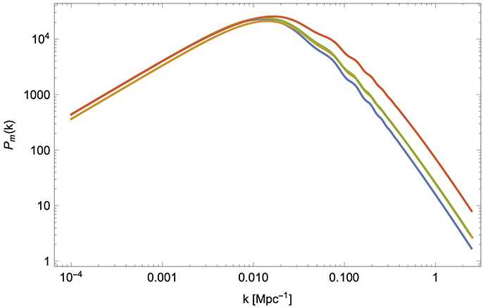
Figure 2. Total matter power spectrum P_m for the same models shown in Figure 1.

As it is for the CMB, these effects can be partly canceled due to parameter degeneracies. Neutrinos, however, have also a peculiar effect on the evolution of matter perturbations. This is due to the fact that neutrinos possess large thermal velocities for a considerable part of the cosmic history, so they can free-stream out of overdense regions, effectively canceling perturbations on small scales. In particular, one can define the free-streaming length at time t as the distance that neutrinos can travel from decoupling until t. The comoving free-streaming length reaches a maximum at the time of the non-relativistic transition. This corresponds to a critical wavenumber k_fs, given in equation (27) for transitions happening during matter-domination, above which perturbations in the neutrino component are erased.

A first consequence of neutrino free-streaming is that, below the free-streaming scale, there is a smaller amount of matter that can cluster. This results in an overall suppression of the power spectrum at small scales, with respect to the neutrinoless case. Secondly, subhorizon perturbations in the non-relativistic (i.e., cold dark matter and baryons) components grow more slowly. In fact, while in a perfectly matter-dominated Universe, the gravitational potential is constant and the matter perturbation grows linearly with the scale factor, δ_m ∝ a, in a mixed matter-radiation Universe the gravitational potential decays slowly inside the horizon. Below the free-streaming scale, neutrinos effectively behave as radiation; then in the limit in which the neutrino fraction f_ν = Ω_ν/Ω_m is small, one has for k ≫ k_fs

$\begin{array}{ll}{\delta }_m(k\gg k_{\text{fs}})\propto a^{1-(3/5)f_{\nu }},& (32)\end{array}$

while δ_m ∝ a for k ≪ k_fs. These two effects can be qualitatively understood as follows: if one considers a volume with linear size well below the free-streaming scale, this region will resemble a Universe with a smaller Ω_m and a larger radiation-to-matter fraction than the “actual” (i.e., averaged over a very large volume) values. This yields a smaller overall normalization of the spectrum, as well as a larger radiation damping; the two effects combine to damp the matter perturbations inside the region. So, looking again at the full power spectrum, the net effect is that, in the presence of free-streaming neutrinos, power at small-scales is suppressed with respect to the case of no neutrinos. At z = 0, the effect saturates at k ≃ 1 h Mpc⁻¹, where a useful approximation is P_m(k, f_ν)/P_m(k, f_ν = 0) ≃ 1−8f_ν [61].

It is useful to stress that since f_ν is linear in Σm_ν, we have the somehow counterintuitive result that the effects of free-streaming are more evident for heavier, and thus colder, neutrinos. The reason is simply that the asymptotic suppression of the spectrum depends only on the total energy density of neutrinos, as this determines the different amount of non-relativistic matter between small and large scales.

Until now, we have somehow ignored the role of baryons in shaping the matter power spectrum. In fact, on scales that enter the horizon after z_drag, the baryons are effectively collisionless and behave exactly like cold dark matter. On the other hand, baryon perturbations at smaller scales, entering the horizon before z_drag exhibit acoustic oscillations due to the coupling with photons. This causes the appearance of an oscillatory structure in the matter power spectrum. These wiggles in P_m(k), that go under the name of baryon acoustic oscillations (BAO), have a characteristic frequency, related to the value of the sound horizon at z_drag. Thus they can serve as a standard ruler and can be used very effectively in order to constrain the expansion history.

In more detail, the acoustic oscillations that set up in the primordial Universe produce a sharp feature in the two-point correlation function of luminous matter at the scale of the sound horizon evaluated at the drag epoch, r_s(z_d) ≡ r_d; this sharp feature translates in (damped) oscillations in the Fourier transform of the two-point correlation function, i.e., the power spectrum. Measuring the BAO feature at redshift z allows in principle to separately constrain the combination d_A(z)/r_d, for measurements in the transverse direction with respect to the line of sight, or r_dH(z) for measurements along the line of sight. An isotropic analysis instead measures, approximately, the ratio between the combination

$\begin{array}{ll}{d}_V(z)={\left[\frac{z{d}_A^2(z)}{H(z)}\right]}^{1/3},& (33)\end{array}$

called the volume-averaged distance, and the sound horizon r_d. Given that the value of the sound horizon is well constrained by CMB observations, measuring the BAO features, possibly at different redshifts, allows to directly constrain the expansion history, as probed by the evolution of the angular diameter distance d_A(z) and of the Hubble function H(z), or of their average d_V(z). In particular, it is straightforward to see that BAO measurements put tight constraints on the Ω_m − H₀r_d plane, along a different degeneracy direction that it is instead probed by CMB [62, 63]. Therefore, when estimating neutrino masses, the addition of BAO constraints to CMB data helps breaking the parameter degeneracies discussed in the previous section, yielding in general tighter constraints on this quantity.

The linear matter power spectrum for a given cosmological model can be computed using a Boltzmann solver. However, comparison with observations is complicated by the non-linear evolution of cosmic structures. Note that both CAMB and CLASS are able to handle non-linearities in the evolution of cosmological perturbations with the inclusion of non-linear corrections from the Halofit model [64] calibrated over numerical simulations. In particular, for cosmological models with massive neutrinos, the preferred prescription is detailed in Bird et al. [65].

From the observational point of view, P_m(k, z) can be probed in different ways. In galaxy surveys, the 3-D spatial distribution of galaxies is measured, allowing to measure the two-point correlation function and to obtain an estimate of the power spectrum of galaxies P_g(k, z). Since in this case one is measuring the distribution of luminous matter only, and not of all matter (including dark matter), this does not necessarily coincide with the quantity for which we have a theoretical prediction, i.e., P_m; in other words, galaxies are a biased tracer of the matter distribution. To take this into account, one relates the two quantities through a bias b(k, z):

$\begin{array}{ll}{P}_g(k,z)=b^2(k,z)P_m(k,z).& (34)\end{array}$

The bias is in general a function of both redshift and scale. If it is approximated as a scale-independent factor, then the presence of the bias only amounts to an overall rescaling of the matter power spectrum (at a given redshift). In this case, one marginalizes over the amplitude of the matter spectrum, effectively only using the information contained in its shape. A scale-independent bias is considered to be a safe approximation for the largest scales: as an example, for Luminous Red Galaxies sampled at an efficient redshift of 0.5 (roughly corresponding to the CMASS sample of the SDSS III-BOSS survey), a scale-independent bias is a good approximation up to k ≲ 0.2 h Mpc⁻¹ [66]. On the other hand, scale-dependent features are expected to appear on smaller scales. In this case, the bias can still be described using a few “nuisance” parameters, that are then marginalized over. In any case the exact functional form of the bias function, the range of scales considered, as well as prior assumptions on the bias parameters, are delicate issues that should be treated carefully. An additional complication arises from the fact that massive neutrinos themselves induce a scale-dependent feature in the bias parameter, due to the scale-dependent growth of structures in cosmologies with massive neutrinos [67, 68].

It has to be mentioned that, at any given redshift, there exists a certain scale k_NL below which the density contrast approaches the limit δ ~ 1. In this regime, the evolution of cosmic structures cannot be completely captured by a linear theory of perturbations. The modeling of structures in the non-linear regime relies on numerical N-body simulations that must take into account the astrophysical and hydrodynamical processes at play at those scales. The level of complexity of N-body simulations has been increasing over the years, so that the physical processes included in the simulations and the final results are much closer to the observations than they used to be at the beginning. Recent examples are given by the MassiveNuS [69] suite, based on the Gadget-2 code [70] modified to include the effects of massive neutrinos, the DEMNUni suite [71–73], the TianNu simulation [74–76], the BAHAMAS project [77], the gevolution simulations [78], and the nuCONCEPT simulations [79] (see also [80] for a method combining the particle and fluid descriptions)⁷. Nevertheless, the uncertainties related to the non-linear evolution of cosmological structures are still higher than those affecting the linear theory, therefore reducing the constraining power coming from the inclusion of those scales in cosmological analysis. In fact, the conservative choice of not including measurements at k > k_NL is usually made when performing cosmological analyses. It is easy to understand that at higher redshifts, a wider range of scales is still in the linear regime.

Additional probes of P_m are measurements of Lyman-α (Lyα) forests and 21-cm fluctuations (see e.g., [83, 84] for reviews). Although they are promising avenues since they can probe the matter distribution at higher redshifts and smaller scales than those usually accessible with typical galaxy samples, they still have to reach the level of maturity required to take full advantage of their constraining power. The observation of high-redshift (z ~ 2) quasars and in particular the measurement of their flux provides a powerful tool for cosmological studies. Indeed, the absorption of the Lyα emission from quasars by the intervening intergalactic medium—an observational feature known as “Lyα forest”—constitutes a tracer of the total matter density field at higher redshifts and smaller scales than those usually probed by galaxy surveys. Similarly to what is done for galaxy samples, one can compute a correlation function of the measured flux variation, or equivalently its power spectrum P_Lyα. The latter is again proportional to the total P_m via a bias parameter b_Lyα. The Lyα bias factor is in general different from the galaxy bias, as each tracer of the underlying total matter distribution exhibits its own characteristics. The Lyα forest is ideally a powerful cosmological tool, being able to access high redshifts. Therefore, at fixed scale k, the physics governing the Lyα spectrum is much closer to the linear regime than that related to the galaxy power spectrum. Furthermore, the redshift window probed by Lyα is complementary to that probed by traditional galaxy surveys, in a sense that at higher redshift the relative impact of dark energy on the cosmic inventory is much smaller. However, a reliable description of the astrophysics at play in the intergalactic medium is essential for deriving the theoretical model for the Lyα absorption features along the line of sight. This description heavily depends on hydrodynamical simulations that reproduce the behavior of baryonic gas and on poorly known details of the reionization history. In addition, uncertainties in the theory of non-linear physics of the intergalactic medium at small scales can play a non-negligible role.

Finally, another tracer of the total matter fluctuations is represented by fluctuations in the 21-cm signal. The 21-cm line is due to the forbidden transition of neutral hydrogen (HI) between the two hyperfine levels of the ground state (spin flip) of the hydrogen atom. The observational technique resides in the possibility to measure the brightness temperature relative to the CMB temperature. Fluctuations in the 21-cm brightness are related to fluctuations in HI (or equivalently to the fraction of free electrons x_e), which in turn trace the matter fluctuations. Therefore, one can infer P_m observationally by measuring the power spectrum of 21-cm fluctuations P_21−cm. Apart from the technological challenges associated with the detection of the 21-cm signal, the main source of systematics come from the difficulties to separate the faint 21-cm signal from the much brighter foreground contamination, mostly due to synchrotron emission from our own galaxy.

4.2.2. Cluster Abundances

The variation of the number of galaxy clusters of a certain mass M with redshift dN(z, M)/dz is also a valid source of information about the evolution of the late time Universe (see e.g., [85] for a review). The expected number of clusters to be observed in a given redshift window is an integral over the redshift bin of the quantity

$\begin{array}{ll}\frac{\text{d}N}{\text{d}z}={\displaystyle \int }\text{d}\Omega {\displaystyle \int }\text{d}M\widehat{\chi }\frac{\text{d}N}{\text{d}M\text{d}z\text{d}\Omega }& (35)\end{array}$

where Ω is the solid angle, $\widehat{\chi }$ is the so-called completeness of the survey (a measure of the probability that the survey will detect a cluster of a given mass M at a given redshift z) and $\frac{\text{d}N}{\text{d}M}(z,M)$ is the mass function giving the number of clusters per unit volume. The latter can be predicted once a cosmological model has been specified. The quantity in Equation (35) is thus directly sensitive to the matter density Ω_m and to the current amplitude of matter overdensities, usually parametrized in terms of σ₈, the variance of matter fluctuations within a sphere of 8 h⁻¹Mpc. As a result, this probe can be highly beneficial for putting bounds on Σm_ν.

Extended catalogs of galaxy clusters have been published in the last decade by the Atacama Cosmology Telescope (ACT) [86, 87], the South Pole Telescope (SPT) [88], and the Planck [24] collaborations. CMB experiments are in fact able to perform searches for galaxy clusters by looking for the thermal Sunyaev-Zeldovich (SZ) effect, the characteristic upward shift in frequency of the CMB signal induced by the inverse-Compton scattering of CMB photons off the hot gas in clusters. The redshift of cluster candidates is identified with follow-up observations, whereas their mass is usually inferred with X-ray observations or, more recently, calibrated through weak lensing. Regardless of how it is calibrated, the determination of the cluster mass is the largest source of uncertainty for the cluster count analysis, due to possibly imprecise assumptions about the dynamical state of the cluster and/or survey systematics. A common way to factorize the uncertainties related to the mass calibration is to introduce a mass bias parameter that relates the true cluster mass to the mass inferred with observations.

4.2.3. Weak Lensing

The weak gravitational lensing effect is the deflection of the light emitted by a source galaxy caused by the foreground large-scale mass distribution (lens). The shape of the source galaxy therefore appears as distorted, i.e., it acquires an apparent ellipticity. The cosmic shear is the weak lensing effect of all the galaxies along the line of sight (see e.g., [89] for a review). Weak lensing surveys offer the possibility to directly test the distribution of intervening matter at low redshifts, thus providing a powerful tool to investigate the late-time evolution of the Universe. By correlating the apparent shapes of source galaxies at different redshifts, one can compute the shear field $\gamma (\widehat{n},z)$ as a function of the angular position $\widehat{n}$ and redshift z. The shear field is usually decomposed in two components: the curl-free E-modes and the divergence-free B-modes. It can be shown that, in absence of systematics, the B-modes are expected to vanish, whereas the power spectrum of the E-modes is equivalent to the lensing power spectrum $C_{\ell }^{\varphi \varphi }$. The integrated lensing potential has been defined in Equation (30) for a source located at recombination. The corresponding expression for a source at a generic redshift z can be obtained simply by substituting χ_∗ with the comoving distance of the source.

Thus, the power spectrum of the lensing potential—which is due to intervening matter along the line of sight—is recovered from the measurements of the lensing-induced ellipticity of background galaxies; in a similar way, the lensing power spectrum is recovered from the redistribution of CMB photons due to the forming structures along the line of sight. As we have seen in section 4.1.1, the spectrum of the lensing potential is a function of the matter power spectrum integrated along the line of sight. Therefore, it carries information about the distribution and growth of structures, representing a powerful tool for constraining Σm_ν. It should be mentioned that the observed shear signal γ_obs is a biased tracer of the true shear γ_true. This effect, mostly due to noise in the pixels when galaxy ellipticity is measured, is usually taken into account by introducing a multiplicative bias m that relates γ_true and γ_obs: γ_obs = (1 + m)γ_true + c, where c is the additional noise bias [90].

In addition, the shear signal can be cross-correlated with the angular distribution of foreground (lens) galaxies (the so-called galaxy-shear or galaxy-galaxy lensing cross-correlation). This cross-correlation is a powerful way to overcome the limitations induced in the galaxy-galaxy auto-correlation by the unknown galaxy bias. Indeed, the galaxy-galaxy lensing is basically a cross-correlation between the galaxy field and the total matter fluctuation field. Measurements of the galaxy-galaxy lensing cross spectrum can therefore help determine the form of the bias.

Cosmological constraints from weak lensing surveys are often summarized in terms of bounds on Ω_m and σ₈. As an additional probe of the large-scale structure in the Universe, weak lensing can be profitably used to constrain Σm_ν.

4.3. Supernovae Ia and Direct Measurements of the Hubble Constant

Measurements of the distance-redshift relation of Supernovae Ia (SNIa) have provided the compelling evidence of the accelerated Universe [91, 92]. SNIa are produced in binary stellar systems in which one of the stars is a white dwarf. Accreting matter from its companion, the white dwarf explodes once it reaches the Chandrasekhar mass limit. Therefore, SNIa are standard candles, because their absolute magnitude can be theoretically inferred from models of stellar evolution. A comparison between the absolute magnitude and the apparent luminosity yields an estimate of their luminosity distance d_L(z). The expected value of d_L in turn depends on the underlying cosmological model. The constraints coming from SNIa in the Ω_m − Ω_Λ plane are orthogonal to those obtained from CMB. As a result, the combination of the two probes is extremely efficient in breaking the degeneracy between the two parameters. For this reason, SNIa are very useful for constraining models of dark energy and/or arbitrary curvature. Nonetheless, constraints on Σm_ν can benefit from the use of SNIa data, thanks to the improved bounds on Ω_m.

As already discussed, the effect of light massive neutrinos on the background evolution of the Universe can be also compensated by a change in the value of the Hubble constant H₀. Therefore, it is clear that any direct measurement of H₀ can be highly beneficial for putting bounds on Σm_ν. Direct measurements only rely on local distance indicators (i.e., redshift z ≪ 1), therefore they are little or not-at-all sensitive to changes in the underlying cosmological model. In contrast, indirect estimates from high-redshift probes, such as primary CMB, can suffer from model dependency.

Direct measurements of H₀ are based on the geometric distance calibration of nearby Cepheids luminosity-period relation and the subsequent calibration of SNIa over Cepheids observed in the same SNIa galaxy hosts (see e.g., [93] and references therein). The goal is to connect the precise geometric distances measured in the nearby Universe (usually referred to as “anchors”) with the distant SNIa magnitude-redshift relation in order to extract the estimate of H₀. The main systematics are of course related to the calibration procedure. Further improvements on the precision of direct measurements of H₀ are expected to come once the precise parallaxes measurements from the Gaia satellite will be available [94].

Local measurements of H₀ are not directly sensitive to Σm_ν. Besides, their results, in combination with cosmological probes, can break the degeneracy between cosmological parameters and improve constraints on Σm_ν. The main example is in fact the possibility to break the strong (inverse) degeneracy between H₀ and Σm_ν that affects CMB constraints.

Indirect estimates of H₀ can be obtained from CMB and BAO measurements. We have already seen in section 4 that the position and amplitude of the first acoustic peak in the CMB spectrum depends on H₀ in combination with other parameters. In addition, we shall mention that, once the BAO are calibrated with the precise determination of r_d from CMB, measurements of d_A/r_d and Hr_d (or d_V/r_d) yields bounds on H₀ that are competitive with CMB estimates and direct measurements.

We finally mention an additional independent measurement of H₀. The gravitational wave (GW) signal emitted by merging compact objects in combination with the observation of an electromagnetic counterpart has been proposed as a standard siren [95, 96]. The GW waveform reconstruction allows for a determination of the luminosity distance to the source. Precise determinations of the source localization can lead to percent accuracy in the luminosity distance estimation. The observation of the electromagnetic counterpart of the GW event is then essential to determine the redshift to the source. The full combination of distance-redshift pair can finally be employed to constrain H₀. In the absence of the detection of an electromagnetic counterpart, methods to infer the redshift of the source of the GW signal have been proposed (see e.g., [97]).

4.4. Summary of the Effects of Neutrino Masses

Before moving to report the current observational constraints, we find it useful to summarize the constraining power of different cosmological observables with respect to the neutrino mass. The discussion is somehow qualitative, also given the high-level complexity of the cosmological models. The purpose is also to underline the importance of combining different cosmological probes.

We start from the CMB. For the present discussion, it is useful to consider separately the information coming from the unlensed CMB (i.e., the primary CMB plus all the secondary effects with the exclusion of lensing) and that coming from the weak lensing of CMB photons. For what concerns the former, the sensitivity of the unlensed CMB to neutrino masses is somehow limited. This is mainly due to a geometrical degeneracy between h and ω_ν thanks to which one can simultaneously change the two parameters (decreasing h and increasing ω_ν) to keep θ_s constant, thus preserving the position of the first peak, with only limited changes to other parts of the spectrum (especially changes in the low-ℓ region, where the sensitivity is limited by cosmic variance, induced by variations in Ω_Λ). The height of the first peak is preserved by keeping ω_c fixed. Having access to the information contained in the CMB lensing, either through its effect on the temperature and polarization power spectra, or through a direct estimation of the lensing power spectrum, helps because Σm_ν also affects the matter distribution and then the amplitude of the lensing potential at small scales. This helps breaking the degeneracy described above.

To illustrate this point, in the upper panel of Figure 3 we show the parameter correlations derived by an analysis of the Planck observations of the temperature, over a wide range of scale, and large-scale polarization anisotropies. We remember that this dataset contains some information about lensing through the high-ℓ part of the temperature power spectrum. The negative degeneracy between Σm_ν and H₀ is particularly evident. Given that ω_c and ω_b are both measured quite well from the CMB, this also translates into a strong degeneracy with ${\Omega }_m=({\omega }_c+{\omega }_b)/h^2$ and Ω_Λ = 1 − Ω_m. Among the other parameters, one can notice mild correlations with A_s and τ. These are due to the small-scale effects related to the increased lensing in models with larger Σm_ν. The overall amplitude of the spectrum $A_s{e}^{-2\tau }$ is very precisely determined by CMB observations. On the other hand, the lensing amplitude depends on A_s but not on τ. So, the lensing amplitude can be kept constant by increasing both A_s and ω_ν. At this point τ has to be increased as well to preserve the scalar amplitude $A_s{e}^{-2\tau }$.

FIGURE 3

Figure 3. Correlation matrices of a selection of cosmological parameters for the combinations of Planck TT+lowP (Upper) and Planck TT+lowP+BAO (Lower). See section 5.1 for the description of these datasets. The darker the color shade, the stronger the degeneracy between the corresponding parameter pair. In both panels, the third row and the third column correspond to the correlation coefficients between Σm_ν and the remaining cosmological parameters. From the comparison between the two panels, it is clear that the inclusion of BAO data helps reduce the degeneracy between parameters (see e.g., the correlation between Σm_ν and H₀, Ω_Λ); in a few cases, in fact, the inclusion of BAO reverts the degeneracy (see e.g., the correlation between Σm_ν and n_s).

Geometric measurements, like those coming from BAO, SNIa, or direct measurements of H₀, greatly help solving the geometrical degeneracy between H₀ and Σm_ν. This is evident in the lower panel of Figure 3, where we show parameter correlations from an analysis of the same dataset as above with the addition of BAO data, if one compares the (H₀, Σm_ν) square with the corresponding square in the upper panel. Measurements of large scale structures, and especially those that are directly sensitive to the total matter distribution at small scales, are very helpful, in that on the one hand they allow to further constrain Ω_m, A_s, and n_s and thus reduce degeneracies with these parameters; on the other hand, they allow to probe the regime in which neutrino free-streaming is important. Finally, it is also clear that a precise measurement of τ from a CMB experiment that is sensitive to the large-scale polarization (meaning that it can access a large fraction of the sky) will be highly beneficial.

We have focused our attention to the ΛCDM + Σm_ν model. In extended dark energy models (as well as modified gravity models), for example for arbitrary equations of state of the dark energy fluid, the degeneracy between Σm_ν and Ω_Λ is amplified. Both massive neutrinos and dark energy-modified gravity affect the late time evolution of the Universe, so that the individual effects on cosmological observables (mostly structures) can be reciprocally canceled.

5. Current Observational Constraints on Σm_ν

In this section we report current constraints on Σm_ν from cosmological and astrophysical observations. These constraints are also summarized in Table 1 for the reader's convenience. Unless otherwise stated, the results are obtained in the framework of a minimal one-parameter extension of the ΛCDM model with varying neutrino mass, dubbed ΛCDM + Σm_ν, in which the three mass eigenstates are degenerate (m_i = Σm_ν/3). Given the sensitivity of current experiments, the degenerate approximation is appropriate. See section 8 for a more detailed discussion on this point.

5.1. CMB

CMB observations are probably the most mature cosmological measurements. The frequency spectrum is known with great accuracy [46]. Measurements of the power spectrum of CMB anisotropies in temperature are cosmic-variance limited down to very small scales (ℓ ~ 1, 500) and the quality of current CMB data in polarization is already good enough to tighten constraints on cosmological parameters [14, 16, 17, 19, 20]. The next generation of CMB experiments will further improve our knowledge of CMB polarization anisotropies [21, 30–33]. The main systematics involved in CMB measurements are due to foreground contamination (atmospheric, galactic, extragalactic), calibration uncertainties and spurious effects induced by an imprecise knowledge of the instrument (see e.g., [108–112] for a sample list of references).

The tightest constraints on Σm_ν from a single experiment come from the measurements of the Planck satellite [14]. In the context of a one-parameter extension of the ΛCDM cosmological model, the state of the art after the 2015 data release was as follows. The combination of the measurements of the CMB temperature anisotropies up to the multipole ℓ ≃ 2, 500 (hereafter, “Planck TT”) and the large scale (ℓ < 30) polarization anisotropies (hereafter “lowP”) leads to an upper bound of Σm_ν < 0.72 eV at 95% CL. The inclusion of the small scale (ℓ ≥ 30) polarization measurements (which we globally label as “Planck TE,EE”) provides a tighter upper bound of Σm_ν < 0.49 eV at 95% CL. This latter bound should be regarded as less conservative, as a small level of residual systematics could still affect the small scale polarization data.

The Planck collaboration also provides the most significant measurements of the CMB lensing potential power spectrum for the multipole range 40 < L < 400 (labeled as “lensing”) [113]. When this dataset is included in the analysis, the 95% CL constraints on Σm_ν become: Σm_ν < 0.68 eV for Planck TT+lowP+lensing and Σm_ν < 0.59 eV for Planck TT,TE,EE+lowP+lensing [14]. When combining the lensing reconstruction data from Planck with the measurements of the CMB power spectra, it should be kept in mind that CMB power spectra as measured by Planck prefer a slightly higher lensing amplitude than that estimated with the lensing reconstruction. As a result, the bounds on Σm_ν obtained by their combination have less weight for smaller values of Σm_ν than the corresponding bounds obtained from CMB power spectra only. Nevertheless, higher values of Σm_ν are still disfavored.

In 2016, new estimates of the reionization optical depth τ have been published by the Planck collaboration [43], obtained from the analysis of the high-frequency CMB maps, in 2015 still affected by unexplained systematics effects at large scales. The estimated 68% credible interval for τ coming from the EE−only low-ℓ data is τ = 0.055 ± 0.009. This estimate is lower than the corresponding interval obtained in 2015 from the analysis of the low-frequency maps (τ = 0.067 ± 0.023), though the two estimates are well in agreement with each other. The lower value of τ has an impact on the constraints on Σm_ν, due to the degeneracy between the optical depth and the amplitude of primordial perturbations A_s, as they together fix the normalization amplitude $A_s{e}^{-2\tau }$. A lower τ implies a lower A_S and thus a lower lensing amplitude, leaving less room for large values of Σm_ν (that would further reduce lensing). If the “lowP” dataset is replaced by the new estimate of τ (labeled as “SimLow”), the 95% CL bounds improve as follows: Σm_ν < 0.59 eV for Planck TT+SimLow and Σm_ν < 0.34 eV for Planck TT,TE,EE+SimLow [43].

5.2. Large-Scale Structure Data

Although the CMB is an extremely powerful dataset, multiple degeneracies between cosmological parameters limit the constraining power on Σm_ν from CMB only, as seen in section 4.4. Measurements of the large scale structures (LSS) can help solving these degeneracies. LSS surveys map the distribution and clustering properties of matter at later times (or equivalently at lower redshift) than those accessible with CMB data and are directly sensitive to cosmological parameters that CMB data can only constrain indirectly, such as the total matter abundance at late times (see e.g., [114] for a review). In this section, we gather constraints on Σm_ν from different LSS probes alone and in combination with CMB data.

5.2.1. Baryon Acoustic Oscillations and the Full Shape of the Matter Power Spectrum from the Clustering of Galaxies

BAO measurements, obtained by mapping the distribution of matter at relatively low redshifts (z < 3) if compared to the redshifts relevant for CMB, constrain the geometry of the expanding Universe, providing estimates of the comoving angular diameter distance d_A(z) and the Hubble parameter H(z) at different redshifts (or an angle-averaged combination of the two parameters, $d_V(z)={\left[z{d}_A^2(z)/H(z)\right]}^{1/3}$). Therefore, BAO constrain cosmological parameters which are relevant for the late-time history of the Universe, helping break the degeneracy between those parameters and Σm_ν.

BAO extraction techniques rely on the ability to localize the peak of the two-point correlation function of some tracer of the baryon density, or equivalently the locations of the acoustic peaks in the matter power spectrum, thus neglecting the information coming from the broad-band shape of the matter power spectrum itself. In principle, the full shape (FS) of the matter power spectrum is a valuable source of information about clustering properties of the different constituents of the Universe and their reciprocal interactions. In particular, full shape measurements of the power spectrum also provide estimates of the growth of structures at low redshifts through the anisotropies induced by the redshift-space distortions (RSD), usually encoded in the parameter f(z)σ₈(z), where f(z) is the logarithmic growth rate and σ₈(z) is the normalization amplitude of fluctuations at a given redshift in terms of rms fluctuations in a 8h⁻¹ Mpc sphere.

In 2016, the final galaxy clustering data from the Baryon Oscillation Spectroscopic Survey (BOSS) were released, as part of the Sloan Digital Sky Survey (SDSS) III⁸. Joint consensus constraints on d_A(z), H(z), and f(z)σ₈(z) from BAO and FS measurements at three different effective redshifts (z_eff = 0.38, 0.51, 0.61) are employed to derive constraints on Σm_ν⁹ in combination with Planck TT,TE,EE+ lowP [23]. The 95% upper bound is Σm_ν < 0.16 eV. When relaxing the constraining power coming from CMB weak lensing (through the rescaling of the lensing potential with the lensing amplitude A_L) and the RSD (through the rescaling of the fσ₈ parameter with the amplitude A_fσ8), the bound degrades up to Σm_ν < 0.25 eV.

When using the FS measurements, it has to be noted that the constraining power of this dataset is highly reduced if one considers that (1) the majority of information encoded in the FS usually comes from the small-scale region of the power spectrum, where the still imprecisely known non-linearities play a non-negligible role; (2) the exact shape and scale-dependence of the bias b between the observed galaxy clustering and the underlying total matter distribution is still debated. Therefore, it is useful to disentangle BAO and FS measurements, to gauge the relative importance of the two in constraining Σm_ν. For a thorough comparison between the constraining power of the two datasets, we refer the reader to Vagnozzi et al. [98] (see also [116, 117] for analyses using older data), where the authors focus on recent BAO and FS measurements. Here, we summarize the conclusion of the paper: “The analysis method commonly adopted [for FS measurements] results in their constraining power still being less powerful than that of the extracted BAO signal.”

5.2.2. Weak Lensing

The most recent weak lensing datasets have been released by the Kilo-Degree Survey (KiDS [26, 118]) and the Dark Energy Survey (DES [27, 119]). It is interesting to note that all of the aforementioned datasets provide results in terms of cosmological parameters which are slightly in tension with the corresponding estimates coming from CMB data (which we remind is a high-redshift probe). In particular, the values of Ω_m and $S_8={\sigma }_8{({\Omega }_m/0.3)}^{0.5}$ inferred from weak lensing data are lower than the best fit obtained with CMB data. The significance of this tension is at ~2σ level for KiDS and more than 1σ level for the 1-D marginalized constraints on Ω_m and S₈ for DES (even though a more careful measure of the consistency between the two datasets in the full parameter space provides “substantial” evidence for consistency, see Abbott et al. [27] for details).

Weak lensing data tend to favor higher values of Σm_ν than those constrained by CMB power spectrum data. In fact, lower values of Ω_m and S₈ imply a reduced clustering amplitude, an effect that can be obtained by increasing the sum of neutrino masses. In Abbott et al. [27], the combination of DES shear, galaxy and galaxy-shear spectra with Planck TT+lowP and other cosmological datasets in agreement with CMB results (i.e., BAO from 6dFGS [100], SDSS DR₇ MGS [104], and BOSS DR12 [23], and luminosity distances from the Joint Lightcurve Analysis (JLA) of distant SNIa [105, 106]) yields an upper bound at 95% CL on the sum of the neutrino masses of Σm_ν < 0.29 eV, almost 20% higher than the corresponding bound obtained dropping DES data (Σm_ν < 0.245 eV). Interestingly enough, the DES collaboration shows that a marginal improvement in the agreement between DES and Planck data is obtained when the sum of the neutrino masses is fixed to the minimal mass allowed by oscillation experiments Σm_ν = 0.06 eV.

To conclude this section, we also report the upper bound on Σm_ν obtained by weak lensing only data from the tomographic weak lensing power spectrum as measured by the KiDS collaboration [26]. They found Σm_ν < 3.3 eV and Σm_ν < 4.5 eV at 95% CL depending on the number of redshift bins retained in the analysis. These bounds are significantly broader than the constraints coming from CMB only data. Nevertheless, they come from independent cosmological measurements and are still tighter than the constraints coming from kinematic measurements of β decay.

5.2.3. Cluster Counts

An additional low-redshift observable is represented by measurements of the number of galaxy clusters as a function of their mass at different redshifts. Cluster number counts provide a tool to infer the present value of the matter density Ω_m and the clustering amplitude σ₈, to be compared with the equivalent quantities probed at higher redshift by the primary CMB anisotropies.

Depending on the prior imposed on the mass bias, cluster counts tend to prefer lower values of Ω_m and σ₈ than the corresponding values obtained with primary CMB. The tension between the two datasets can be as high as 3.7σ for the lowest value of the mass bias as quantified by the Planck collaboration in 2015 [24]. Again, this preference for less power in the matter distribution favors higher values of the sum of the neutrino masses. Indeed, the Planck collaboration reports [24] an upper bound of Σm_ν < 0.20 eV at 95% CL when Planck TT,TE,EE+lowP+BAO is combined with the SZ cluster count dataset (with a prior on the mass bias (1−b) = 0.780 ± 0.092 from the gravitational shear measurements of the Canadian Cluster Comparison Project, CCCP [120]), to be compared with the corresponding 95% upper bound Σm_ν < 0.17 eV without the SZ cluster count dataset [14].

Recently, Salvati et al. [121] updated constraints on cosmological parameters, including Σm_ν, from the SZ clusters in the Planck SZ catalog, considering cluster count alone and in combination with the angular power spectrum of SZ sources. A comparison with bounds coming from primary CMB anisotropies is also performed. The combination of the two SZ probes (complemented with BAO measurements from [102] to fix the underlying cosmology) confirms the discrepancy in Ω_m and σ₈ at the level of 2.1σ and provides an independent upper limit on the sum of the neutrino masses of Σm_ν < 1.47 eV at 95% CL. When combined with primary CMB, the bound reduces to Σm_ν < 0.18 eV. This bound is slightly higher than Σm_ν < 0.12 eV found by Vagnozzi et al. [98] in absence of SZ data, as we should expect due to the aforementioned tension between SZ and primary CMB estimates of matter density and power.

5.2.4. Lyman-α Forests

Like all the datasets that probe the clustering of matter over cosmological distances, the Lyα power spectrum is sensitive to Σm_ν primarily through the power suppression induced by massive neutrinos at small scales. The Lyα spectrum alone can constrain Σm_ν at the level of 1 eV (see e.g., [107]). The constraining power of the Lyα spectrum is evident when it is combined with CMB data. In this case, the Lyα data are used for setting the overall normalization of the spectrum through their sensitivity to Ω_m and σ₈, whereas the CMB fixes the underlying cosmological parameters and helps break degeneracies between Ω_m, σ₈, and Σm_ν. Recently, Yèche et al. [122] reported constraints on Σm_ν from the combination of the one-dimensional (i.e., angle-averaged) Lyα power spectra from the SDSS III-BOSS collaboration and from the VLT/XSHOOTER legacy survey (XQ- 100). When the power spectra are used alone [complemented with a Gaussian prior on $H_0=(67.3\pm 1.0)\text{ km }{\text{s}}^{-1}\text{Mp}{\text{c}}^{-1}$], the authors obtain Σm_ν < 0.8 eV at 95% CL. The bounds dramatically improve to Σm_ν < 0.14 eV when CMB power spectrum data from Planck TT+lowP are added to the analysis. The tightest bound on Σm_ν from Lyα power spectrum comes from Palanque-Delabrouille et al. [107], with Σm_ν < 0.12 eV from Planck TT+lowP in combination with the Lyα flux power spectrum from BOSS-DR12. Interestingly enough, in both analyses, the limit set by Lyα+Planck TT+lowP does not further improve when the Lyα spectra are combined instead with the full set of CMB data from Planck, including small-scale CMB polarization (Planck TT,TE,EE+lowP), and with BAO data from 6dFGS, SDSS MGS, BOSS-DR11.

The BAO signal can be also extracted from the Lyα spectrum (see [123] for a pivotal study), providing estimates of the comoving angular diameter distance d_A(z) and of the Hubble parameter H(z) at redshift z ≃ 2. Recently, the SDSS III-BOSS DR12 collaboration reported measurements of the BAO signal at z = 2.33 from Lyα forest [99]. The estimated values of d_A and H are in agreement with a ΛCDM model (even though a slight tension with Planck primary CMB is present), although their precision is smaller than the precision obtained with galaxy-derived BAO measurements. Therefore, at present, the impact of Lyα-BAO data on simple extensions of the ΛCDM model is minimal.

We conclude that it is a conservative choice to take the constraints coming from Lyα with some caution (a similar comment applies to constraints coming from aggressive analyses of the broadband shape of the matter power spectrum from galaxy surveys), until this probe will reach the level of maturity comparable with other traditional cosmological probes.

5.3. Local Measurements of the Hubble Constant and Supernovae Ia

The most recent estimate of the Hubble constant has been reported in Riess et al. [93]. The authors improved over their previous measurement of H₀ from 3.3 to 2.4% thanks to an increased sample of reliable SNIa in nearby galaxies calibrated over Cepheids. Their final estimate, based on the combination of three different anchors, is $H_0=(73.24\pm 1.74)\text{ km }{\text{s}}^{-1}\text{Mp}{\text{c}}^{-1}$, 3.2σ higher than the indirect estimate of H₀ from Planck TT+SimLow (3.4σ higher than Planck TT,TE,EE+SimLow) in the context of a ΛCDM cosmology with Σm_ν = 0.06 eV. Previous analyses from the same authors also pointed to a ~2σ tension between direct measurements of H₀ and indirect estimate from primary CMB anisotropies from Planck (although see [124] for a re-analysis of the same dataset which slightly reduces the discrepancy to within 1σ agreement). A discussion about the possible reasons behind this discrepancy and ways to alleviate it invoking non-standard cosmological scenarios are beyond the scope of this work. We refer the reader to the dedicated works [62, 125, 126] for further reading.

Since the Hubble constant and the sum of neutrino masses are anti-correlated, given the tension between the two probes it is clear that the combination of direct measurements of H₀ with CMB data leads to a preference for smaller values of Σm_ν with respect to CMB-only constraints. Indeed, several authors have pointed out the tight constraints on Σm_ν for such a combination. As an example, Vagnozzi et al. [98] showed that constraints on Σm_ν can be as tight as Σm_ν < 0.148 eV at 95% CL when Planck TT+lowP+BAO are complemented with a Gaussian prior on H₀ equal to the estimate of the Hubble constant in Riess et al. [93], to be compared with Σm_ν < 0.186 eV from Planck TT+lowP+BAO only. When lowP is replaced by a Gaussian prior on τ compatible with the new estimates from SimLow, these numbers change to Σm_ν < 0.115 eV (Σm_ν < 0.151 eV) with (without) the H₀ prior.

For the sake of completeness, we shall also mention that independent estimates of H₀ from BAO measurements conducted by the SDSS III-BOSS DR12 collaboration [23] are in agreement with CMB estimates (see also [62] for a recent discussion). See also Abbott et al. [127] for an additional independent estimate of H₀ with a combination of clustering and weak lensing measurements from DES-Y1 with BAO and BBN data. A discussion about the combination of different measurements of H₀ from cosmological probes and local measurements is also reported in Abbott et al. [127], Vega-Ferrero et al. [128].

Finally, we report that a standard siren measurement of H₀ has been performed after the detection of the neutron star-neutron star merger GW170817 [129–131]. The Hubble constant has been constrained as $H_0=70.0_{-8.0}^{+12.0}\text{ km }{\text{s}}^{-1}\text{Mp}{\text{c}}^{-1}$ at 68% CL. The accuracy of this determination is not comparable with the precise estimates of direct measurements and other cosmological constraints. However, the standard siren approach represents an additional independent estimate of H₀ and appears as a promising avenue as more GW events with electromagnetic counterparts are detected.

Concerning the inclusion of SNIa, the bounds from Planck TT+lowP improve from Σm_ν < 0.72 eV to Σm_ν < 0.33 eV at 95% CL when data from the Joint Lightcurve Analysis [105, 106] are included¹⁰. The most relevant systematics that affect SNIa measurements are related to the way in which SNIa light curves are standardized, with issues mostly arising from photometric calibrations and lightcurve fitting procedures.

6. Constraints on Σm_ν from Future Surveys

In this section, we will discuss the expected improvements in the constraints on Σm_ν from the upcoming generation of CMB and LSS surveys. These constraints are also summarized in Table 2 for the reader's convenience.

TABLE 2

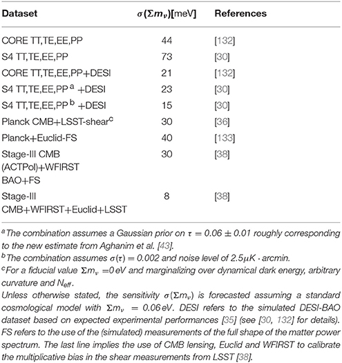
Table 2. Expected sensitivity on Σm_ν from different combination of future cosmological data.

6.1. CMB Surveys: CORE and CMB Stage-IV

The tightest bounds on Σm_ν from a single CMB experiment are those from the Planck satellite, reported in section 5.1. As already explained, this sensitivity mostly comes from the ability to (1) detect, at the level of CMB power spectrum, the smoothing effect of gravitational lensing of CMB photons, and, (2) directly reconstruct the lensing power spectrum itself. These effects arise at small angular scales (higher multipoles ℓ), therefore it is crucial to observe this region of the power spectrum with high accuracy in order to improve the sensitivity on Σm_ν. Improved measurements of the polarization power spectra at all scales are also important to break degeneracies between cosmological parameters. The main example is the effect that a better estimate of the reionization optical depth τ from the large scale polarization spectrum has on Σm_ν. Concerning the lensing power spectrum, this is internally reconstructed by the Planck collaboration with high statistical significance up to intermediate scales. However, the full power of this probe will be definitively unveiled when better measurements of polarization maps are available, enabling reconstruction from E-B estimators with lower variance and up to smaller scales [57].

A detailed summary of the expected sensitivity to cosmological parameters, including Σm_ν, of all pre-2020 and post-2020 CMB missions can be found in Errard et al. [134]. As relevant examples, in this section we focus on two classes of future (post 2020) CMB experiments: a space mission and a ground based telescope.

Recently, a proposal for a future CMB space mission has been submitted to the European Space Agency (ESA) in response to a call for medium-size mission proposals (M5). The mission, named Cosmic ORigin Explorer (CORE), is designed to have 19 frequency channels in the range 60−600 GHz for simultaneously solving for CMB and foreground signals, angular resolution in the range 2′−18′ depending on the frequency channel and aggregate sensitivity of 2 μK·arcmin [32] (for comparison, the Planck satellite has 9 frequency channels in the range 30−900 GHz, angular resolution in the range 5′−33′ and the most sensitive channel shows a temperature noise of 0.55 μK·deg at 143 GHz [135]). This experimental setup would enable to constrain $\Sigma m_{\nu }=(0.072_{-0.051}^{+0.037})\text{ eV}$ at 68% CL assuming a ΛCDM model with a fiducial value of the sum of the neutrino masses Σm_ν = 0.06 eV, for the combination of CORE TT,TE,EE,PP (temperature and E-polarization auto and cross spectra and lensing power spectrum PP) [132]. This roughly corresponds to a sensitivity of σ(Σm_ν) ~ 0.044 eV (note that the target threshold for a 3σ detection in the minimal mass scenario is σ(Σm_ν) = 0.020 eV; for comparison, a simulated Planck-like experiment could only put an upper limit of Σm_ν < 0.315 eV at 68% CL for the same model). Other than to the capability of measuring with high precision the small scale polarization (also in order to reconstruct the lensing potential), part of this high sensitivity also comes from the improved limits that a science mission like CORE can put on τ: compared to Planck, CORE would achieve an almost cosmic-variance-limited (CVL) detection of the reionization optical depth [σ_CVL(τ) ≃ 0.002].

A roadmap towards a Stage-IV (S4) generation of CMB ground-based experiments¹¹ has been also developing [30]. The goal is to set a definitive CMB experiment with ~250,000 detectors surveying half of the sky, with angular resolution of 1′ − 2′ and a sensitivity of 1μK·arcmin at 150 GHz. The greatest contaminant for a ground-based experiment is the atmospheric noise, which highly reduces the accessible frequencies for CMB observations to a total of four windows, roughly 35, 90, 150, and 250 GHz. The main advantages with respect to a space-borne mission are a larger collecting area with an incredibly higher number of detectors (for a comparison, the CORE proposal accounts for a total of 2,100 detectors [32], the Planck satellite has 74 detectors [135]) and subsequent suppression of experimental noise. At large scales, the Stage-IV target is the recombination bump at ℓ > 20. The reduced sky fraction accessible from ground, foreground contaminations and atmospheric noise are the main issues that limit the possibility to target also the range ℓ < 20. Therefore, it is likely that S4 would be complemented by balloon-based and satellite-based measurements at the largest scales. As a result, forecasts for S4 relies on external measurements of τ. The sensitivity σ(Σm_ν) of S₄ TT,TE,EE,PP complemented with a Gaussian prior on the optical depth of τ = 0.06 ± 0.01 (roughly corresponding to the latest estimate from Planck-HFI [43]) is in the range [0.073 − 0.110] eV, depending on the angular resolution and noise level, for f_sky = 40% [30].

Neither of the two classes of future CMB mission proposals can achieve alone the necessary sensitivity to claim a detection of Σm_ν = 0.06 eV at the 3-σ level. Nevertheless, we will see in the next section that the combination of future CMB missions with future galaxy surveys could possibly lead to the first detection of neutrino masses from cosmology.

6.2. Future LSS Surveys: DESI, Euclid, LSST, WFIRST

Improved performances from future galaxy surveys with respect to the current status can be achieved by mapping a larger volume of the sky, therefore increasing the number of samples observed and going deeper in redshift. In this section, we will briefly review the expected performances of the main Stage-IV LSS surveys.

The successor to SDSS III-BOSS survey will be the ground-based Dark Energy Spectroscopic Instrument¹² (DESI). It is designed to operate for 5 years and cover roughly a 14,000 deg² survey area. The extension in redshift is expected to be up to z = 1 for Luminous Red Galaxies (LRG), z = 1.7 for Emission Line Galaxies (ELG) and z = 3.5 for Lyα forests, for a total of over 20 million galaxy and quasar redshifts. With these numbers, DESI will improve over the BOSS survey by an order of magnitude in both volume covered and number of objects observed. It can achieve a 3.49% and 4.78% determination of the BAO signal across (d_A/r_d) and along (Hr_d) the line-of-sight, respectively, at z = 1.85, and 16% and 9% determination of the same quantities at the highest redshift achievable with Lyα forest z = 3.55 [35]. Even in the most conservative scenario when DESI BAO only (i.e., without including information from the broadband shape of the matter power spectrum and Lyα forests) are combined with future CMB experiments, the sensitivity on Σm_ν greatly improves. It goes down to σ(Σm_ν) = 0.021 eV for CORE TT,TE,EE,PP+DESI BAO, forecasting a ~3σ detection of Σm_ν in the minimal mass scenario [132]. In the case of S4+DESI BAO [30], σ(Σm_ν) is in the range [0.023 − 0.036] eV (or [0.020 − 0.032] eV) with a prior of τ = 0.06 ± 0.01 (or τ = 0.060 ± 0.006, the expected sensitivity from Planck-HFI [136]) and f_sky = 0.40, depending on the S4 angular resolution and noise level. For a 1′ resolution and a noise level lower than 2.5 μK · arcmin, σ(Σm_ν) could be further improved with a better measurement of τ down to the level of σ(Σm_ν) < 0.015 eV, that would guarantee a >4σ detection of Σm_ν in the minimal mass scenario.

The DESI mission will be complementary to the science goals of the Large Synoptic Survey Telescope¹³ (LSST), a Stage-IV ground-based optical telescope. The main science fields in which LSST will mostly operate are [36]: “Inventory of the Solar System, Mapping the Milky Way, Exploring the Transient Optical Sky, and Probing Dark Energy and Dark Matter”. These goals will be achieved by surveying a ~30,000 deg² area (2/3 of which in a “deep-wide-fast” survey mode) over 10 years, in six bands (ugrizy), with incredible angular resolution (~ 0.7″), producing measurements of roughly 10 billion stars and galaxies. Thanks to its peculiar observational strategy, LSST will provide multiple probes of the late-time evolution of the Universe with a single experiment, namely, weak lensing cosmic shear, BAO in the galaxy power spectrum, evolution of the mass function of galaxy clusters, and a compilation of SNIa redshift-distances. The expected sensitivity on Σm_ν [36] is in the range σ(Σm_ν) = [0.030 − 0.070] eV, depending on the fiducial value of Σm_ν assumed when performing forecasts ($\Sigma m_{\nu }^{\text{fid}}=\left[0-0.66\right]\text{ eV}$). Larger fiducial values for the mass yield better sensitivity. These numbers include a marginalization over the uncertainties coming from an extended cosmological scenario, where a number of relativistic species different than 3.046, a non-zero curvature and a dynamical dark energy component are allowed. They also take into account the combination of the three-dimensional cosmic shear field as measured by a LSST-like survey with Planck-like CMB data and can be improved by a factor of 2 if either BAO or SNIa measurements are also considered, whereas a factor of $\sqrt{2}$ degradation could come from systematic effects. Interestingly enough, the observational strategy of LSST (large and deep survey) could provide the necessary sensitivity to explore the faint effects that the distinct neutrino mass eigenstates have on cosmological probes. This is a highly debated topic and we refer the reader to section 8 for related discussion.

Synergy between these large ground-based observatories and future space missions is expected. We consider here the ESA Euclid satellite¹⁴ and the NASA Wide Field Infrared Survey Telescope¹⁵ (WFIRST) as representative space-borne missions. Euclid will be a wide-field satellite that operates with imaging and spectroscopic instruments for 6 years and covers roughly 15,000 deg² in the optical and near-infrared bands, observing a billion galaxies and measuring ~100 million galaxy redshifts [37]. The redshift depth will be up to z ~ 2 for galaxy clustering and up to z ~ 3 for cosmic shear. The combination of the galaxy power spectrum measured with Euclid and primary CMB from Planck is expected to give σ(Σm_ν) = 0.04 eV; if instead the weak lensing dataset produced by Euclid is considered in combination with primary CMB, we expect σ(Σm_ν) = 0.05 eV [133]. Both combinations provide a ~ 1σ evidence in the minimal mass scenario. Some authors have also pointed out that weak lensing data as measured by Euclid could discriminate between the two neutrino hierarchies if the true value of Σm_ν is small enough (i.e., far enough from the degenerate region of the neutrino mass spectrum), see [133] and references therein¹⁶.

WFIRST is an infrared telescope with a primary mirror as wide as the Hubble Space Telescope's primary (2.4 m) and will operate for 6 years [38]. The primary instrument on board, the Wide Field Instrument, will be able to operate both in imaging and spectroscopic mode, observing a billion galaxies. The instrumental characteristics of WFIRST will more than double the surface galaxy density measured by Euclid. With this setup, WFIRST will test the late expansion of the Universe with great accuracy employing supernovae, weak lensing, BAO, redshift space distortions (RSD), and clusters as probes. From the BAO and broadband measurements of the matter power spectrum, WFIRST in combination with a Stage-III CMB experiment could provide σ(Σm_ν) < 0.03 eV [38].

We want to conclude this section by pointing out that the aforementioned missions will be extremely powerful if combined together. Indeed, they are quite complementary [137]. A significant example concerning the improvement of constraints on massive neutrinos is the combination of all the previously discussed surveys with the lensing reconstruction from CMB. The cross correlation of weak lensing (optical), CMB lensing power spectrum and galaxy clustering (spectroscopic) can highly reduce the systematics affecting each single probe, in particular the multiplicative bias in cosmic shear [138]. For example, a combination of WFIRST, Euclid, LSST, and CMB Stage-III can achieve σ(Σm_ν) < 0.01 eV [38]. Another example is the calibration of the cluster mass for SZ cluster count analyses. This calibration can be performed through optical surveys such as LSST or through CMB lensing calibration, with comparable results. In Madhavacheril et al. [139], the authors show that lensing-calibrated SZ cluster counts can provide a detection of the minimal neutrino mass Σm_ν at > 3σ level, also in extended cosmological scenarios.

6.3. 21-cm Surveys

In this section, we will briefly comment about the possibility to use 21-cm survey data to constrain Σm_ν. We refer the reader to the relevant papers for further readings. Measurements of the 21-cm signal such as those expected from the Square Kilometer Array¹⁷ (SKA) and the Canadian Hydrogen Intensity Mapping Experiment¹⁸ (CHIME) can shed light on the Epoch of Reionization, including a better determination of the reionization optical depth τ. In addition, they map the distribution of neutral hydrogen in the Universe, a tracer of the underlying matter distribution. Therefore, constraints on Σm_ν can benefit from 21-cm measurements in two ways: by breaking the degeneracy between Σm_ν and τ (see e.g., [140], where the authors report σ(Σm_ν) = 0.012 eV for a combination of CORE+Euclid lensing and FS+ a prior on τ compatible with expectations from future 21-cm surveys); by detecting the effect of Σm_ν on the evolution of matter perturbations (see e.g., [141–143]).

7. Constraints on Σm_ν in Extended Cosmological Scenarios

The constraints reported so far apply to the simple one-parameter extension of the standard cosmological model, ΛCDM + Σm_ν. When derived in the context of more complicated scenarios, such as models that allow arbitrary curvature and/or non-standard dark energy models and/or modified gravity scenarios etc., constraints on Σm_ν are expected in general to degrade (although tighter constraints on Σm_ν can be also possible in particular extended scenarios) with respect to those obtained in a ΛCDM + Σm_ν cosmology. This effect is due to the multiple degeneracies arising between cosmological parameters that describe the cosmological model under scrutiny. In other words, when more degrees of freedom are available—in terms of cosmological parameters that are not fixed by the model—, more variables can be tuned in order to adapt the theoretical model to the data. For example, CMB data measure with incredible accuracy the location (expressed by the angular size of the horizon at recombination θ_s) and amplitude (basically driven by the exact value of z_eq) of the first acoustic peak. Therefore, we want to preserve this feature in any cosmological model. As explained before, h, Ω_m, and Σm_ν can be varied together in order to do this. Adding other degrees of freedom, like curvature or evolving dark energy, allows for even more freedom, thus making the degeneracy worse. Of course, the addition of different cosmological data, which are usually sensitive to different combinations of the aforementioned parameters, is extremely helpful in tightening the constraints on Σm_ν (and, in general, on any other cosmological parameter) in complex scenarios.

In more detail, constraints on the sum of neutrino masses are particularly sensitive to the so-called “geometric degeneracy.” This term refers to the possibility of adjusting the parameters in order to keep constant the angle subtended by the sound horizon at last scattering, that controls the position of the first peak of the CMB anisotropy spectrum. The degeneracy is worsened in models with a varying curvature density Ω_k or parameter of the equation of state of dark energy w. Constraints on the expansion history, like those provided by BAO or by direct measurements of the Hubble constant, are particularly helpful in breaking the geometric degeneracy. In principle, one could also expect a degeneracy between the effective number of degrees of freedom N_eff and Σm_ν, but for a different reason: both parameters can be varied in order to keep constant the redshift of matter-radiation equality. However, this can be done only at the expense of changing the CMB damping scale (see section 10 for further details). High-resolution measurements of the CMB anisotropies are therefore a key to partially break the degeneracy. Finally, a non-standard relation between the matter density distribution and the lensing potential can be modeled by introducing a phenomenological parameter A_L, which modulates the amplitude of the lensing signal [144]. Most of the current constraining power of CMB experiments on Σm_ν comes from CMB lensing. Therefore, it is clear that in models with varying A_L the limits on neutrino masses are strongly degraded. However, it should also be noted that A_L is usually introduced as a proxy for instrumental systematics; if considered as an actual physical parameter, its value is fixed by general relativity to be A_L = 1.

To make the discussion more quantitative, we see how this applies to the constraints obtained with present data and future data. In Table 3, we report a comparison of the constraints on Σm_ν for some extensions of the ΛCDM model. In the upper part of the table, we report constraints obtained from the PlanckTT+lowP+lensing+BAO dataset combination, described in section 5.1. These are taken from the full grid of results made available by the Planck collaboration¹⁹ and have been obtained with the same statistical techniques used for the ΛCDM model. We see that the constraints are degraded by 30% in models with varying N_eff, by 50% in models with varying Ω_K or w, and by 65% in models with varying A_L. This information is also conveyed, for an easier visual comparison, in Figure 4, where we show the sum of neutrino masses as a function of the mass m_light of the lightest eigenstate. The green and red curves are for normal and inverted hierarchy, respectively. We show 95% constraints on Σm_ν for different models and dataset combinations as horizontal lines. In the lower section of Table 3 we instead report a similar comparison, based on the expected sensitivities of future CMB and LSS probes [132]. The pattern is very similar to that observed for present data, although it should be noted that the increased precision of future experiments will allow to further reduce the degeneracies. In particular, it is found that the constraints on Σm_ν are degraded by ~30% in models with varying Ω_K or w, and not degraded at all in models with varying N_eff (models with varying A_L have not been considered in Di Valentino et al. [132]).

TABLE 3

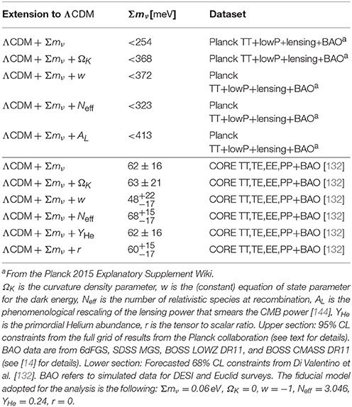
Table 3. Constraints on Σm_ν from different extensions to the ΛCDM model for the indicated datasets.

FIGURE 4

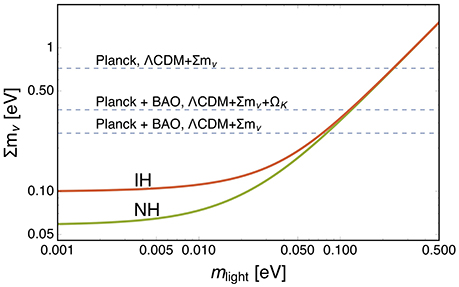
Figure 4. Sum of neutrino masses Σm_ν as a function of the mass m_light of the lightest neutrino eigenstate, for normal (green) or inverted (red) hierarchy. The horizontal dashed lines show 95% CL upper limits for different dataset combinations, from top to bottom: PlanckTT+lowP in the ΛCDM + Σm_ν model, PlanckTT+lowP+BAO in the ΛCDM + Σm_ν + Ω_K model, PlanckTT+lowP+BAO in the ΛCDM + Σm_ν model.

The cases reported in Table 3 hardly exhaust all the possible, well-motivated extensions to the ΛCDM + Σm_ν model. To make a few examples of more complicated extensions, without the aim of being complete, the interplay between inflationary parameters and the neutrino sector has been investigated in Gerbino et al. [145] and Di Valentino et al. [146]. In Di Valentino et al. [147–149] “extended parameter spaces” are considered, in which 12 parameters, including Σm_ν, are varied simultaneously. Neutrino-dark matter interactions are discussed in Di Valentino et al. [150], while low-reheating scenarios are studied in de Salas et al. [151]. Finally, constraints on Σm_ν in the context of cosmological models with time-varying dark energy are derived for example in Lorenz et al. [152] and Yang et al. [153]. Neutrino masses in interacting dark energy-dark matter models and in extended neutrino models (including neutrino viscosity, anisotropic stress and lepton asymmetry) have instead been considered in Kumar and Nunes [154] and in Nunes and Bonilla [155].

8. Cosmology and the Neutrino Mass Hierarchy

Cosmology is mostly sensitive to the total energy density in neutrinos, directly proportional to the sum of the neutrino masses Σm_ν ≡ m₁ + m₂ + m₃. We can express Σm_ν in the two hierarchies as a function of the lightest eigenstate m_light (either m₁ or m₃) and of the squared mass differences $\Delta m_{12}^2$ and $\Delta m_{13}^2$:

$\begin{array}{l}\Sigma m_{\nu }^{NH}=m_{\text{light}}+\sqrt{m_{\text{light}}^2+\Delta m_{12}^2}\\ +\sqrt{m_{\text{light}}^2+|\Delta m_{13}^2|}& (36)\end{array}$

$\begin{array}{l}\Sigma m_{\nu }^{IH}=m_{\text{light}}+\sqrt{m_{\text{light}}^2+|\Delta m_{13}^2|}\\ +\sqrt{m_{\text{light}}^2+|\Delta m_{13}^2|+\Delta m_{12}^2}& (37)\end{array}$

When stating that oscillation experiments are insensitive to the absolute mass scale, one refers to the fact that the value of m_light is not accessible with oscillation data. When m_light = 0 eV, one obtains $\Sigma m_{\nu }^{NH}\simeq 0.06\text{ eV}$ and $\Sigma m_{\nu }^{IH}\simeq 0.1\text{ eV}$. Therefore, for each hierarchy, a minimum mass scenario exists in which Σm_ν ≠ 0.

It has been a long-standing issue whether or not cosmological probes are sensitive to the neutrino mass hierarchy. In principle, we expect physical effects on cosmological observables due to the choice of the neutrino hierarchy. Individual neutrino species that carry a slightly different individual mass exhibit a slightly different free-streaming scale k_fs: depending on their individual mass, neutrinos can finish suppressing the matter power at different epochs, leaving three distinct “kinks” in the matter power spectrum. As a consequence, the weak lensing effects on the CMB and on high redshift galaxies can be slightly affected by the choice of the hierarchy. In practice, all of these signatures are at the level of permille effects on the matter and CMB power spectra, well below the current sensitivity [156].

Given the current sensitivity (roughly Σm_ν < 0.2 eV at 95% CL), it is then a legitimate assumption to approximate the mass spectrum as perfectly degenerate (m_i = Σm_ν/3) when performing analysis of cosmological data. Very recently, several authors investigated the possibility that such an approximation could fail reproducing the physical behavior of massive neutrinos when observed with the high sensitivity of future cosmological surveys [132, 145, 157, 158]. In addition, the issue of whether future surveys could unravel the unknown hierarchy has been addressed by several groups [98, 158–162]. We refer the reader to the relevant papers for a thorough discussion of these issues. Here, we summarize the main results: (1) the sensitivity of future experiments will not be enough to clearly separate the effects of different choices of the neutrino hierarchy, for a given value of Σm_ν; therefore the fully-degenerate approximation is still a viable way to model the neutrino mass spectrum in the context of cosmological analysis; (2) the possibility to clearly identify the neutrino hierarchy with future cosmological probes is related to the capability of measuring Σm_ν < 0.1 eV at high statistical significance, in order to exclude the IH scenario. It is clear that the possibility to do this strongly depends on the true value of Σm_ν: the closer it is to $\Sigma m_{\nu }^{NH}=0.06\text{ eV}$, the larger will be the statistical significance by which we can exclude IH. This is true independently of whether we approach the issue from a frequentist or Bayesian perspective. In the latter case, however, since a detection of the hierarchy would be driven by volume effects, this posits the question of what is the correct prior choice for Σm_ν. The issue is extensively discussed in Gerbino et al. [159], Simpson et al. [163], Schwetz et al. [164], Caldwell et al. [165], Long et al. [166], and Hannestad and Tram [167].

9. Complementarity with Laboratory Searches

Cosmological observables are ideal probes of the neutrino absolute mass scale, though they are not the only probes available. In fact, laboratory avenues such as kinematic measurements in β-decay experiments (see e.g., [168]) and neutrino-less double-β decay (0ν2β) searches (see e.g., [169, 170]) provide complementary pieces of information to those brought by cosmology.

Kinematic measurements are carried on with β-decay experiments mostly involving ³H. The shape of the decay spectrum close to the end point is sensitive to the (electron) neutrino mass and can be parametrized in terms of constraints on the electron neutrino effective mass²⁰ defined in Equation (12). The current best limits on m_β come from the Troitzk and Mainz experiments, with m_β < 2.05 eV [1] and m_β < 2.3 eV [2] at 95% CL. The new generation ³H β-decay experiment KATRIN (Karlsruhe Tritium Neutrino²¹) is expected either to reach a sensitivity of m_β < 0.2 eV at 90% CL, an order of magnitude improvement with respect to current sensitivities, or to detect the neutrino mass if it is higher than m_β = 0.35 eV. Note that a detection of non-zero neutrino mass in KATRIN would imply Σm_ν ≳ 1 eV, and would then be in tension with the cosmological constraints obtained in the framework of the ΛCDM model. This could point to the necessity of revising the standard cosmological model, although it should be noted that none of the simple one-parameter extensions reported in Table 3 could accommodate for such a value.

Future improvements in kinematic measurements involve technological challenges, since KATRIN reaches the experimental limitations imposed to an experiment with spectrometers. Future prospects are represented by the possibility of calorimetric measurements of ¹³⁶Ho (HOLMES experiment [171]) and measurements of the ³H decay spectrum via relativistic shift in the cyclotron frequency of the electrons emitted in the decay (Project8 experiment²² [172]). Although the bounds coming from β-decay experiments are very loose compared to bounds from cosmology, nevertheless they are appealing for the reason that they represent model-independent constraints on the neutrino mass scale, only relying on kinematic measurements.

0ν2β decay is a rare process that is allowed only if neutrinos are Majorana particles. A detection of 0ν2β events thus would solve the issue related to the nature of neutrinos, whether they are Dirac or Majorana particles. Searches for 0ν2β directly probe the number of 0ν2β events, which is related to the half life T_1/2 of the isotope involved in the decay. The half life can be translated in limits on the Majorana mass m_ββ (defined in Equation 13) once a nuclear model has been specified. In practice, a bound on T_1/2 is reflected in a range of bounds on m_ββ, due to the large uncertainties associated with the exact modeling of the nuclear matrix elements. Additional complications are due to model dependencies: when translating bounds on T_1/2 to bounds on m_ββ, a mechanism responsible for the 0ν2β decay has to be specified. This is usually the exchange of light Majorana neutrinos, though alternative mechanisms could be responsible for the lepton number violation that not necessarily allow a direct connection between T_1/2 and m_ββ. Finally, it can be shown that in the case of NH, disruptive interference between mixing parameters could prevent a detection of 0ν2β events, regardless of the neutrino nature and the lepton-number violation mechanism.

We report here some of the more recent limits on m_ββ from 0ν2β searches. Constraints are reported as a range of 90% CL upper limits, due to the uncertainty on the nuclear matrix elements. We also specify the isotope used in each experiment. The current bounds are m_ββ < 0.120−0.270 eV from Gerda Phase-II (⁷⁶Ge) [173, 174], m_ββ < 0.061−0.165 eV from KamLAND-Zen [175] (¹³⁶Xe), m_ββ < 0.147−0.398 eV from EXO-200 (¹³⁶Xe) [176], m_ββ < 0.140−0.400 eV from CUORE (¹³⁰Te) [177]. The next generation 0ν2β experiments, such as LEGEND, SuperNEMO, CUPID, SNO+, KamLAND2-Zen, nEXO, NEXT, PANDAX-III, aims to cover the entire region of IH, reaching a 3σ discovery sensitivity for m_ββ of 20 meV or better, roughly an order of magnitude improvement with respect to the current limits (see [178] for a more detailed discussion and for a full list of references).

As outlined above, laboratory searches and cosmology are sensitive to different combinations of neutrino mixing parameters and individual masses. Therefore, it makes sense to compare their performances in terms of constraints on the neutrino mass scale. It is also beneficial to combine these different probes of the mass scale, in order to overcome the limitations of each single probe and increase the overall sensitivity to the neutrino masses [40, 165, 179]. This is possible because, once the elements of the mixing matrix are known, specifying one of three mass parameters among (m_β, m_ββ, Σm_ν), together with the solar and atmospheric mass splittings, uniquely determines the other two. Oscillation experiments measure precisely the values of the mixing angles and of the squared mass differences, with an ambiguity on the sign of $\Delta m_{31}^2$, so that these parameters can be simply fixed to their best-fit values, given the larger uncertainties on the absolute mass parameters. The value of the Dirac phase, on the other hand, is known with lesser precision, and the Majorana phases, relevant for the interpretation of 0ν2β searches, are not probed at all by oscillation experiments. However this ignorance can be folded into the analysis using standard statistical techniques. Finally, the relation between the mass parameters also depends on the mass hierarchy. This can be taken into account either by performing different analyses for NH and IH, or by marginalizing over the hierarchy itself (see e.g., [159]).

Combining the different probes of the absolute mass scale, with the support of oscillation results, leads to some interesting considerations. First of all, basically all of the information on the absolute mass scale comes from cosmology and 0ν2β searches. This confirms the naive expectation that can be made by comparing the sensitivity of the different probes. However, we recall again that the robust limits on m_β from kinematic experiments represent an invaluable test for the consistency of the more model-dependent constraints coming from cosmology and 0ν2β decay experiments. At the moment, cosmology still provides most of the information on the neutrino masses, although the sensitivity of 0ν2β experiments is rapidly approaching that of cosmological observations. A summary of the current limits is reported in Figure 3 of Gerbino et al. [159]. To better illustrate the complementarity of cosmology and 0ν2β searches, we show in Figure 5 how they constrain, together with oscillation experiments, the allowed space in the (m_ββ, m_light) plane. In more detail, we show the region in that plane that is singled out by oscillation experiments, for normal and inverted hierarchy. The width of the allowed regions traces the uncertainties on the CP-violating phases. We show current upper 95% bounds on m_ββ from 0ν2β searches as horizontal lines, and current 95% bounds on m_light from cosmology as vertical lines. These are translated from the bounds on Σm_ν using information from oscillation experiments and assuming normal hierarchy. Assuming inverted hierarchy would however make a barely noticeable difference on the scale of the plot. It can be seen that in general cosmological observations are more constraining than 0ν2β searches.

FIGURE 5

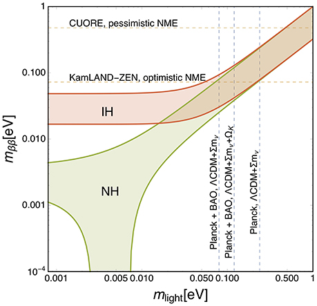
Figure 5. Majorana mass m_ββ of the electron neutrino as a function of the mass m_light of the lightest neutrino eigenstate, for normal (green) or inverted (red) hierarchy. The filled regions correspond to the uncertainty related to the CP-violating phases. The horizontal dashed lines show 95% current upper limits from 0ν2β searches. In particular, we show the tightest and loosest limits among those reported in the text, namely the most stringent from KamLAND-Zen (labeled “KamLAND-Zen, optimistic NME”), and the less stringent from CUORE (labeled “CUORE, pessimistic NME”). NME refers to the uncertainty related to the nuclear matrix elements. We also show vertical dashed lines corresponding to 95% upper limits on Σm_ν from cosmological observations, translated to upper limits on m_light using the information from oscillation experiments. In particular we show different model and dataset combinations, from right to left: PlanckTT+lowP in the ΛCDM + Σm_ν model, PlanckTT+lowP+BAO in the ΛCDM + Σm_ν + Ω_K model, PlanckTT+lowP+BAO in the ΛCDM + Σm_ν model. The vertical lines shown in the plot assume normal hierarchy, but the difference with the case of inverted hierarchy is very small on the scale of the plot.

In the future, however, one can expect that the constraining power of these two probes will be roughly equivalent. This can be seen in Figure 6 where, similarly to Figure 5, we show the allowed space in the (m_ββ, m_light) plane for future cosmological and 0ν2β probes. As shown in Gerbino et al. [159], the constraining power of 0ν2β searches for Σm_ν would also depend crucially on the possibility of reducing the uncertainty on the nuclear matrix elements for the 0ν2β isotopes. In fact, provided that neutrinos are Majorana particles and that the leading mechanism responsible for the decay is a mass mechanism, the combination of cosmological probes and 0ν2β measurements could not only lead to a detection of the mass scale, but could also solve the hierarchy dilemma and provide useful information about (at least one of) the Majorana phases [179–181].

FIGURE 6

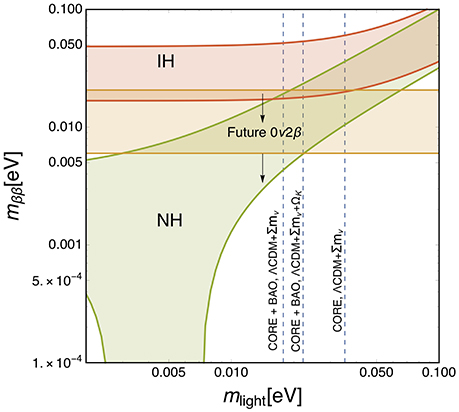
Figure 6. The same as Figure 5, but for future cosmological observations and 0ν2β experiments. Note that in this figure we show 95% upper limits for both m_ββ and m_light, assuming that the true values of both quantities are much smaller that the corresponding experimental sensitivities. The horizontal yellow band labeled “Future 0ν2β” is the union of the regions that contain the 95% upper limits for LEGEND 1K, CUPID, and nEXO, assuming 5 years of live time. The vertical dashed lines correspond to 95% upper limits on Σm_ν. From right to left: CORE TT, TE, EE, PP in the ΛCDM + Σm_ν model, CORE TT, TE, EE, PP + the DESI and EUCLID BAO in the ΛCDM + Σm_ν + Ω_K model, CORE TT, TE, EE, PP + the DESI and EUCLID BAO in the ΛCDM + Σm_ν model. The vertical lines shown in the plot assume normal hierarchy.

10. Constraints on N_eff

Until now, we have focused on the capability of cosmological observations to constrain neutrino masses. However, as noted in the introduction, cosmology is also a powerful probe of other neutrino properties. The main example is without any doubt the effective number of neutrino families (also called effective number of relativistic degrees of freedom) N_eff, defined in Equation (21). As it is clear from its definition, N_eff is simply a measure of the total cosmological density during the radiation-dominated era. More precisely, it represents the density in relativistic species, other than photons, normalized to the energy density of a massless neutrino that decouples well before electron-positron annihilation (that, we remember, is not actually the case). As explained in section 2.5, the standard framework, in which photons and active neutrinos are the only relativistic degrees of freedom present, and neutrino interactions follow the SM of particle physics, predicts N_eff = 3.046 after electron-positron annihilation [12, 47, 48].

Given its meaning, it is clear that a deviation from the expected value of N_eff can hint to a broad class of effects—in fact, all those effects that change the density of light species in the early Universe. Those effects are not necessarily related to neutrino physics, as the definition of N_eff in terms of the number of relativistic degrees of freedom suggests. For example, the existence of a Goldstone boson that decouples well before the QCD phase transition would appear as an increased number of degrees of freedom, with ΔN_eff ≡ N_eff − 3.046 = 0.027 [182]. Speaking however about changes in N_eff that are somehow related to neutrino physics, the most notable example is probably the existence of one (or more) additional, sterile light eigenstate, produced through some mechanism in the early Universe. In such a situation, one would have N_eff > 3.046, as well as an additional contribution to Σm_ν. Note that a light sterile neutrino would not necessarily contribute with ΔN_eff = 1, as it does not share the same temperature as the active neutrinos.

In this section we will focus on cosmological constraints on sterile neutrinos. However, for completeness, we mention a few other examples of scenarios in which ΔN_eff can possibly be different from zero. One is the presence of primordial lepton asymmetries, related to the presence of a non-vanishing chemical potential in the neutrino distribution function, Equation (15). Constraints on the allowed amount of lepton asymmetry, obtained taking into account the effect of neutrino oscillations, have been reported in Castorina et al. [183] using CMB and BBN data. Another possibility is the so-called low-reheating scenario [151, 184, 185], in which the latest reheating episode of the Universe happens just before BBN, at temperatures of the order of a few MeV, so that neutrinos do not have time to thermalize completely. In this case, one has ΔN_eff ≤ 0. Finally, non-standard interactions between neutrino and electrons can modify the time of neutrino decoupling [186], so that the entropy transfer from e⁺e⁻ annihilation and N_eff are different with respect to the standard picture. We note that the effects related to these new scenarios are often more complicated that just a change in N_eff: for example, both in the case of lepton asymmetries and low reheating, the neutrino distribution function is changed in a non-trivial way, affecting also the other moments of the distribution (like the number density, the average velocity, etc.). Finally, to mention a possibility that is not related to changes in N_eff, cosmology can also probe the free-streaming nature of neutrinos, for example by looking for the effects of non-standard interactions among neutrinos [187–190], or between neutrinos and dark matter [191–193].

Let us briefly recall how N_eff is constrained by cosmological observations [194]. Increasing N_eff will make the Universe expand faster (larger H) during the radiation-dominated era, and thus be younger at any given redshift. Then the comoving sound horizon at recombination will be smaller, going like 1/H, while the angular diameter distance to recombination stays constant, because H is unchanged after equality, so that θ_s is smaller. Also, for fixed matter content, this will make the radiation-dominated era last longer. Recalling our discussion in section 4.1, the effect on the CMB spectrum is that the first peak is enhanced due to the larger early ISW, and all the peaks are moved to the right. However, as we have already learned, these effects can be canceled by acting on other parameters. There is however a more subtle and peculiar effect of N_eff, that is related to the scale of Silk damping. The damping scale roughly scales as $1/\sqrt{H}$, i.e., as $\sqrt{t}$, as expected for a random walk process. Then the ratio between the angle subtended by the sound horizon and that subtended by the damping length scales like H⁻¹/H^−1/2 = H^−1/2. Since θ_s is fixed by the position of the first peak, this means that, when increasing N_eff, the damping length is projected on larger angular scales, or, equivalently, that damping at a given scale is larger. In conclusion the net effect is to lower the damping tail of the CMB spectrum. This effect is difficult to mimic with other parameters, at least in the standard framework. The damping length also depends on the density of baryons, so in principle one could think of changing this to compensate for the effect of N_eff; however, the baryon density is very well determined by the ratio of the heights of the first and second peak, so that it is in practice fixed. One possibility, in extended models, is to vary the fraction of primordial helium. Since the mean free path of photons depends on the number of free electrons, and helium recombines slightly before hydrogen, changing the helium-to-hydrogen ratio alters the Silk scale. However, this requires the assumption of non-standard BBN, since, in the framework of standard BBN, the helium fraction is fixed by ω_b and N_eff themselves, so it is not a free parameter.

We first review constraints on N_eff in a simple one-parameter extension of ΛCDM, in which N_eff is left free to vary, and the mass of active neutrinos is kept fixed to the minimum value allowed by oscillations. This case can be considered as the most agnostic, in some sense, in which one does not make any hypothesis on the new physics that is changing N_eff (and thus on any other effects this new physics might produce). Moreover, one can think of these as limits for a very light (massless) sterile neutrino. Finally, constraining N_eff is a robustness check for the standard ΛCDM model. In fact, measuring N_eff = 3.046 within the experimental uncertainty can be seen as a great success of the standard cosmological model. It can be regarded as an indirect detection of the CνB, or, at least, of some component who has the same density, within errors, as we would expect for the three active neutrinos²³. From PlanckTT+lowP, one gets N_eff = 3.13 ± 0.32; adding BAO gives N_eff = 3.15 ± 0.23 [14]. Both measurements, with a precision of ~10%, are in excellent agreement with the standard prediction. Moreover, according to these results, ΔN_eff = 1 is excluded at least at the 3σ level. Using also information about the full shape of the matter power spectrum, the BOSS collaboration finds N_eff = 3.03 ± 0.18 [23]. We note that adding information from direct measurements of the Hubble constant results in larger values of N_eff (N_eff = 3.41 ± 0.22 from Planck TT,TE,EE+lowP+lensing+BAO+JLA+H₀, see [93]); this is due to the tension with the value of H₀ that is inferred from the CMB, that is alleviated in models with larger N_eff. The next generation of cosmological experiments will improve these constraints by roughly one order of magnitude, getting close to the theoretical threshold of ΔN_eff = 0.027 discussed at the beginning of this section, corresponding to a Goldstone boson decoupling before the QCD phase transition. Moreover, it will be possible to confirm the effects of non-instantaneous decoupling, since future sensitivities will allow to distinguish, at the 1-σ level, between N_eff = 3 and N_eff = 3.046. The combination of CORE TT,TE,EE,PP will put an upper bound at 68% CL of ΔN_eff < 0.040 on the presence of extra massless (m ≪ 0.01 eV) species²⁴ [132] in addition to the three active neutrino families. The CORE collaboration puts limits also on the scenario in which the three active neutrinos have a fixed temperature, but their energy density is rescaled as ${(N_{\text{eff}}/3.046)}^{3/4}$. This scenario can account for an enhanced neutrino density (if N_eff > 3.046) and reduced neutrino density (if N_eff < 3.046 as for example in the case of low-reheating scenarios). In this case, CORE TT,TE,EE,PP yields N_eff = 3.045 ± 0.041. Forecasts from S4 show that, in order to get closer to the threshold of ΔN_eff = 0.027, a sensitivity of 1μK·arcmin and f_sky > 50% are needed for a 1′ beam size [30]. Efficient de-lensing will help improve the limits on N_eff: delensed spectra will have sharper acoustic peaks, allowing to constrain N_eff not only through the impact on the Silk scale, but also through the phase shift in the acoustic peaks [195]. Finally, having access to a larger sky fraction—and therefore to a larger number of modes observed—will be beneficial for constraints on N_eff [30]. We conclude this summary about future limits by noticing that the inclusion of LSS data, such as BAO measurements from DESI and Euclid, provides only little improvements with respect to CMB-only constraints (e.g., from CORE TT,TE,EE,PP+DESI BAO+Euclid BAO, ΔN_eff < 0.038 at 68% CL for extra massless species and N_eff = 3.046 ± 0.039 for three neutrinos with rescaled energy density [132]). For a summary of current and future limits on N_eff, we refer to Table 4.

TABLE 4

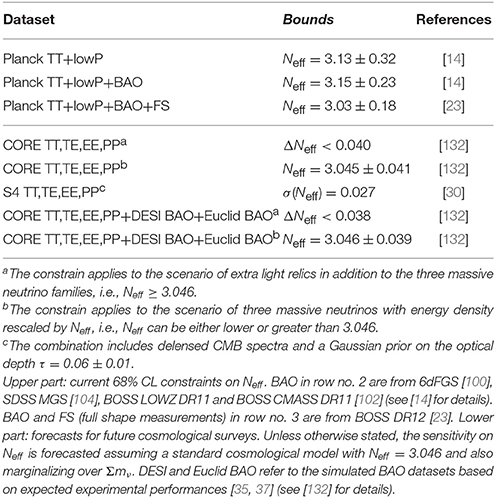
Table 4. Constraints on N_eff (at 68% CL) from different combinations of cosmological data.

Let us now come to the case of a massive sterile neutrino. A sterile neutrino would contribute both to N_eff and to ω_ν. Its effect on the cosmological observables will thus be related to changes in these two quantities, as explained through this review. In fact, in principle, we should specify the full form of the distribution function of the sterile neutrino, and its effects could not be fully parameterized through N_eff and ω_ν. Fortunately, one has that, when the distribution function is proportional to a Fermi-Dirac distribution, all the effects on the perturbation evolution of a light fermion can be mapped into two parameters [196]: its energy density in the relativistic limit (and thus its contribution to N_eff) and its energy density in the non-relativistic limit (and thus its density parameter, let us denote it with ω_s to distinguish it from the active neutrinos). This covers several physically interesting cases, namely those of a sterile neutrino that either (i) has a thermal distribution with arbitrary temperature T_s, or (ii) is distributed proportionally to the active neutrinos, but with a suppression factor χ_s (this corresponds to the Dodelson-Widrow (DW) prediction for the non-resonant production scenario [197]; see also Merle et al. [198]). Defining an effective mass $m_s^{\text{eff}}$ by mimicking Equation 19, i.e.,

$\begin{array}{ll}{m}_s^{\text{eff}}\equiv 93.14{\omega }_s\text{ eV},& (38)\end{array}$

the actual mass m_s of the sterile is related to the effective parameters by:

$\begin{array}{ll}{m}_s={(T_s/T_{\nu })}^{-3}{m}_s^{\text{eff}}=\Delta N_{\text{eff}}^{-3/4}{m}_s^{\text{eff}}(\text{thermal})& (39)\end{array}$

$\begin{array}{ll}{m}_s={\chi }_s^{-1}{m}_s^{\text{eff}}=\Delta N_{\text{eff}}^{-1}{m}_s^{\text{eff}}(\text{DW}).& (40)\end{array}$

Planck data are consistent with no sterile neutrinos: the 95% allowed region in parameter space is N_eff < 3.7, $m_s^{\text{eff}}<0.52\text{ eV}$ from PlanckTT + lowP + lensing + BAO. However, it should be noted that they do not exclude a sterile neutrino, provided its contribution to the total energy density is small enough. A light sterile neutrino has been proposed as an explanation of the anomalies observed in short-baseline (SBL) experiments (see e.g., [199] and references therein). However, a sterile neutrino with the mass (m_s ≃ 1 eV) and coupling required to explain reactor anomalies would rapidly thermalize in the early Universe (see e.g., [200, 201]) and lead to ΔN_eff = 1, strongly at variance with cosmological constraints (excluded at more than 99% confidence considering the above combination of Planck and BAO data). We conclude this section by quoting the forecasts for future cosmological probes. In the context of a ΛCDM + Σm_ν model with $\Sigma m_{\nu }^{\text{fid}}=0.06\text{ eV}$ and $m_s^{\text{fid}}=0\text{ eV}$, the combination of CORE TT,TE,EE,PP with BAO measurements from DESI and Euclid will provide ΔN_eff < 0.054 and m_s < 0.035 eV [132].

11. Summary

The absolute scale of neutrino masses is one of the main open questions in physics to date. Measuring the neutrino mass could shed light on the mechanism of mass generation, possibly related to new physics at a high energy scale. From the experimental point of view, neutrino masses can be probed in the laboratory, with β- and double β-decay experiments, and with cosmological observations. In fact, cosmology is at the moment the most sensitive probe of neutrino masses. Upper limits from cosmology on the sum of neutrino masses are possibly based on combinations of different observables. Results from the CMB alone can be regarded as very robust: these are of the order of Σm_ν < 0.7 eV (95% CL). The addition of geometrical measurements, like those provided by BAO—also very robust—brings down this limit to Σm_ν < 0.2 eV (95% CL). More aggressive analyses can get the bound very close to the minimum value allowed by oscillation experiments in the case of inverted hierarchy, but are based on observations where control of systematics is more difficult and thus should be taken with caution. It should also be borne in mind that cosmological inferences of neutrino masses are somehow model dependent. In extended cosmological models, especially those involving non-vanishing spatial curvature or dark energy, the constraints on Σm_ν are degraded, even though they still remain very competitive with those obtained from laboratory experiments. Combination of future CMB and LSS experiments could reach, if systematics are kept under control, a sensitivity of 15 meV in the first half of the next decade, allowing a 4σ detection of neutrino masses if the hierarchy is normal and the lightest eigenstate is massless. In that case, it will also be possible to exclude the inverted hierarchy scenario with a high statistical significance.

Present data are also compatible with the standard description of the neutrino sector, based on the standard model of particle physics. CMB measurements constrain the number of relativistic species at recombination to be N_eff = 3.13 ± 0.32 at 68% CL. The inclusion of LSS data further tightens the constraints to N_eff = 3.03 ± 0.18 at 68% CL. These results exclude the presence of an additional thermalized species at more than 3σ level. Cosmological data are also consistent with no sterile neutrinos. Thus no new physics in the neutrino sector is presently required to interpret cosmological data. The standard picture will be tested more thoroughly by future experiments, that will allow to probe to an unprecedented level the physics of neutrino decoupling. An example would be the possibility to constrain non-standard neutrino-electron interactions. Future cosmological probes will also possibly reach the sensitivity necessary to detect, at the 1-σ level, the increase in the number of degrees of freedom due to a Goldstone boson that decouples well before the QCD phase transition.

Author Contributions

Both authors listed have made a substantial, direct and intellectual contribution to the work, and approved it for publication.

Conflict of Interest Statement

The authors declare that the research was conducted in the absence of any commercial or financial relationships that could be construed as a potential conflict of interest.

The reviewer SP declared a past co-authorship with one of the authors ML to the handling Editor.

Acknowledgments

We thank Carmelita Carbone, Francesco Forastieri, Keir Rogers, Sunny Vagnozzi for useful comments about the manuscript. MG acknowledges support by the Vetenskapsrådet (Swedish 3493 Research Council) through contract No. 638-2013-8993 and the 3494 Oskar Klein Centre for Cosmoparticle Physics. ML acknowledges support from INFN through the InDark and Gruppo IV fundings, and from ASI through the Grant 2016-24-H.0 (COSMOS) and through the ASI/INAF Agreement I/072/09/0 for the Planck LFI Activity of Phase E2. We would like to thank the University of Ferrara and the Oskar Klein Centre for kind hospitality.

Footnotes

1. ^https://simonsobservatory.org

2. ^All throughout this review, we take c = ℏ = k_B = 1.

3. ^We choose not to rescale K to make it equal to ±1 for an open or closed Universe, so that we are left with the freedom to rescale the scale factor today a₀ to unity.

4. ^In the analysis of CMB data, the angle subtended by the sound horizon at recombination is normally used in place of h, as it is measured directly by CMB observations, see section 4.1.

5. ^We are assuming a vanishing chemical potential for neutrinos and antineutrinos, i.e., a vanishing lepton asymmetry.

6. ^We are assuming that the lensing field is isotropic.

7. ^Prescriptions for the matter power spectrum in the non-linear regime are also provided by the Halofit model [65], the Coyote Universe emulator [81], the semi-analytical approach of PINOCCHIO [82], and additional methods referenced in Rizzo et al. [82].

8. ^Recently, the DES collaboration has reported a 4% measurement of the angular diameter distance from the distribution of galaxies to redshift z = 1 [115]. Cosmological constraints are derived in the ΛCDM framework, with Σm_ν fixed to the minimal value of 0.06 eV. Therefore, no bounds on Σm_ν have been extracted from the BAO measurements from DES yet.

9. ^Note that the authors follow the assumption that all the mass is carried by only one of three neutrino species, i.e., m₁ = Σm_ν, m_2,3 = 0 eV, instead of the more widely used fully-degenerate approximation of m_i = Σm_ν/3, i = 1, 2, 3 for each of the three neutrino species.

10. ^Bounds from the Planck Legacy Archive: https://wiki.cosmos.esa.int/planckpla2015/index.php/Cosmological_Parameters

11. ^https://cmb-s4.org

12. ^http://desi.lbl.gov

13. ^https://www.lsst.org

14. ^https://www.euclid-ec.org

15. ^https://wfirst.gsfc.nasa.gov

16. ^Note that the specifics of the Euclid mission have changed since the time when [133] was published. The new specifics are not publicly available, however the Euclid collaboration is expected to release updated forecasts in the near future.

17. ^http://skatelescope.org

18. ^https://chime-experiment.ca

19. ^The full grid can be downloaded from the Planck Legacy Archive.

20. ^It has to be noticed that the observable which β-decay experiments are sensitive to is $m_{\beta }^2$, rather than m_β. Nevertheless, it is useful to quote constraints in terms of m_β to facilitate the comparison with results from other probes.

21. ^https://www.katrin.kit.edu

22. ^http://www.project8.org/index.html

23. ^The fact that, when probed, there is no hint for deviations from the free-streaming behavior should strengthen our belief that we are really observing the CνB.

24. ^This constraint has been obtained in the context of a ΛCDM + Σm_ν cosmology, with $\Sigma m_{\nu }^{\text{fid}}=0.06\text{eV}$.

References

1. Aseev VN, Belesev AI, Berlev AI, Geraskin EV, Golubev AA, Likhovid NA, et al. An upper limit on electron antineutrino mass from Troitsk experiment. Phys Rev D (2011) 84:112003. doi: 10.1103/PhysRevD.84.112003

CrossRef Full Text | Google Scholar

2. Kraus Ch, Bornschein B, Bornschein L, Bonn J, Flatt B, Kovalik A, et al. Final results from phase II of the Mainz neutrino mass search in tritium beta decay. Eur Phys J C (2005) 40:447–68. doi: 10.1140/epjc/s2005-02139-7

CrossRef Full Text | Google Scholar

3. Osipowicz A, Blumer H, Drexlin G, Eitel K, Meisel G, Plischke P, et al. KATRIN: A Next generation tritium beta decay experiment with sub-eV sensitivity for the electron neutrino mass. Lett Intent. arXiv: hep-ex/0109033.

4. Schechter J, Valle JWF. Neutrinoless Double beta Decay in SU(2) x U(1) Theories. Phys Rev D (1982) 25:2951–4. doi: 10.1103/PhysRevD.25.2951

CrossRef Full Text | Google Scholar

5. Mohapatra RN, Senjanovic G. Neutrino mass and spontaneous parity violation. Phys Rev Lett. (1980) 44:912–5. doi: 10.1103/PhysRevLett.44.912

CrossRef Full Text | Google Scholar

6. Schechter J, Valle JWF. Neutrino Masses in SU(2) x U(1) Theories. Phys Rev D (1980) 22:2227–35. doi: 10.1103/PhysRevD.22.2227

CrossRef Full Text | Google Scholar

7. Lazarides G, Shafi Q, Wetterich C. Proton lifetime and fermion masses in an SO(10) model. Nucl Phys B. (1981) 181:287–300. doi: 10.1016/0550-3213(81)90354-0

CrossRef Full Text | Google Scholar

8. Chikashige Y, Mohapatra RN, Peccei RD. Are there real goldstone bosons associated with broken lepton number? Phys Lett. (1981) 98B:265–8. doi: 10.1016/0370-2693(81)90011-3

CrossRef Full Text | Google Scholar

9. Schechter J, Valle JWF. Neutrino decay and spontaneous violation of lepton number. Phys Rev D (1982) 25:774–83. doi: 10.1103/PhysRevD.25.774

CrossRef Full Text | Google Scholar

10. Lesgourgues J, Mangano G, Miele G, Pastor S. Neutrino Cosmology. Cambridge, UK: Cambridge University Press (2013).

Google Scholar

11. Betts S, Blanchard WR, Carnevale RH, Chang C, Chen C, Chidzik S, et al. Development of a relic neutrino detection experiment at PTOLEMY: princeton tritium observatory for light, early-universe, massive-neutrino yield. arXiv: 1307.4738 [astro-ph.IM].

12. Dolgov AD. Neutrinos in cosmology. Phys Rept. (2002) 370:333–535. doi: 10.1016/S0370-1573(02)00139-4

CrossRef Full Text | Google Scholar

13. Lesgourgues J, Pastor S. Massive neutrinos and cosmology. Phys Rept. (2006) 429:307–79. doi: 10.1016/j.physrep.2006.04.001

CrossRef Full Text | Google Scholar

14. Ade PAR, Aghanim N, Arnaud M, Ashdown M, Aumont J, Baccigalupi C, et al. Planck 2015 results. XIII. Cosmological parameters. Astron Astrophys. (2016) 594:A13. doi: 10.1051/0004-6361/201525830

CrossRef Full Text | Google Scholar

15. Hinshaw G, Larson D, Komatsu E, Spergel DN, Bennett CL, Dunkley J, et al. Nine-year Wilkinson Microwave Anisotropy Probe (WMAP) observations: cosmological parameter results. Astrophys J. (2012) 208:19. doi: 10.1088/0067-0049/208/2/19

CrossRef Full Text | Google Scholar

16. Louis T, Grace E, Hasselfield M, Lungu M, Maurin L, Addison GE, et al. The Atacama cosmology telescope: two-season ACTPol spectra and parameters. JCAP (2017) 1706:031. doi: 10.1088/1475-7516/2017/06/031

CrossRef Full Text | Google Scholar

17. Henning JW, Sayre JT, Reichardt CL, Ade PAR, Anderson AJ, Austermann JE, et al. Measurements of the Temperature and E-Mode Polarization of the CMB from 500 Square Degrees of SPTpol Data. Astrophys J. arXiv: 1707.09353 [astro-ph.CO].

18. Ade PAR, Ahmed Z, Aikin RW, Alexander KD, Barkats D, Benton SJ, et al. BICEP2/Keck Array VIII: measurement of gravitational lensing from large-scale B-mode polarization. Astrophys J. (2016) 833:228. doi: 10.3847/1538-4357/833/2/228

CrossRef Full Text | Google Scholar

19. Ade PAR, Ahmed Z, Aikin RW, Alexander KD, Barkats D, Benton SJ, et al. Improved constraints on cosmology and foregrounds from BICEP2 and keck array cosmic microwave background data with inclusion of 95 GHz band. Phys Rev Lett. (2016) 116:031302. doi: 10.1103/PhysRevLett.116.031302

PubMed Abstract | CrossRef Full Text | Google Scholar

20. Ade PAR, Aguilar M, Akiba Y, Arnold K, Baccigalupi C, Barron D, et al. A measurement of the cosmic microwave background B-mode polarization power spectrum at sub-degree scales from 2 years of POLARBEAR data. Astrophys J. (2017) 848:121. doi: 10.3847/1538-4357/aa8e9f

CrossRef Full Text | Google Scholar

21. Essinger-Hileman T, Ali A, Amiri M, Appel JW, Araujo D, Bennett CL, et al. CLASS: the cosmology large angular scale surveyor. Proc SPIE Int Soc Opt Eng. (2014) 9153:91531I. doi: 10.1117/12.2056701

CrossRef Full Text | Google Scholar

22. Fraisse AA, Ade PAR, Amiri M, Benton SJ, Bock JJ, Bond JR, et al. SPIDER: probing the early Universe with a suborbital polarimeter. JCAP (2013) 1304:047. doi: 10.1088/1475-7516/2013/04/047

CrossRef Full Text | Google Scholar

23. Alam S, Ata M, Bailey S, Beutler F, Bizyaev D, Blazek JA, et al. The clustering of galaxies in the completed SDSS-III Baryon Oscillation Spectroscopic Survey: cosmological analysis of the DR12 galaxy sample. Mon Not Roy Astron Soc. (2017) 470:2617–52. doi: 10.1093/mnras/stx721

CrossRef Full Text | Google Scholar

24. Ade PAR, Aghanim N, Arnaud M, Ashdown M, Aumont J, Baccigalupi C, et al. Planck 2015 results. XXIV. Cosmology from Sunyaev-Zeldovich cluster counts. Astron Astrophys. (2016) 594:A24. doi: 10.1051/0004-6361/201525833

CrossRef Full Text | Google Scholar

25. Heymans C, Van Waerbeke L, Miller L, Erben T, Hildebrandt H, Hoekstra H, et al. CFHTLenS: the Canada-France-Hawaii telescope lensing survey. Mon Not Roy Astron Soc. (2012) 427:146–66. doi: 10.1111/j.1365-2966.2012.21952.x

CrossRef Full Text | Google Scholar

26. Köhlinger F, Viola M, Joachimi B, Hoekstra H, van Uitert E, Hildebrandt H, et al. KiDS-450: the tomographic weak lensing power spectrum and constraints on cosmological parameters. Mon Not Roy Astron Soc. (2017) 471:4412–35. doi: 10.1093/mnras/stx1820

CrossRef Full Text | Google Scholar

27. Abbott TMC, Abdalla FB, Alarcon A, Aleksić J, Allam S, Allen S, et al. Dark energy survey year 1 results: cosmological constraints from galaxy clustering and weak lensing. arXiv: 1708.01530 [astro-ph.CO].

28. Henderson SW, Allison R, Austermann J, Baildon T, Battaglia N, Beall JA, et al. Advanced ACTPol cryogenic detector arrays and readout. J Low Temp Phys. (2016) 184:772–9. doi: 10.1007/s10909-016-1575-z

CrossRef Full Text | Google Scholar

29. Benson BA, Ade PAR, Ahmed Z, Allen SW, Arnold K, Austermann JE, et al. SPT-3G: a next-generation cosmic microwave background polarization experiment on the south pole telescope. Proc SPIE Int Soc Opt Eng. (2014) 9153:91531P. doi: 10.1117/12.2057305

CrossRef Full Text | Google Scholar

30. Abazajian KN, Adshead P, Ahmed Z, Allen SW, Alonso D, Arnold KS, et al. CMB-S4 Science Book, 1st Edn. arXiv: 1610.02743 [astro-ph.CO].

31. Suzuki A, Ade P, Akiba Y, Aleman C, Arnold K, Baccigalupi C, et al. The POLARBEAR-2 and the simons array experiment. J Low Temp Phys. (2016) 184:805–10. doi: 10.1007/s10909-015-1425-4

CrossRef Full Text | Google Scholar

32. Delabrouille J, de Bernardis P, Bouchet FR, Achúcarro A, Ade PAR, Allison R, et al. Exploring cosmic origins with CORE: survey requirements and mission design. arXiv: 1706.04516 [astro-ph.IM].

33. Matsumura T, Akiba Y, Borrill J, Chinone Y, Dobbs M, Fuke H, et al. Mission design of LiteBIRD. J Low Temp Phys. (2014) 176:733–40. doi: 10.1007/s10909-013-0996-1

CrossRef Full Text | Google Scholar

34. Kogut A, Fixsen DJ, Chuss DT, Dotson J, Dwek E, Halpern M, et al. The Primordial Inflation Explorer (PIXIE): a nulling polarimeter for cosmic microwave background observations. JCAP (2011) 1107:025. doi: 10.1088/1475-7516/2011/07/025

CrossRef Full Text | Google Scholar

35. Science Final Design Report. Available online at: http://desi.lbl.gov/tdr/

36. Abell PA, Allison J, Anderson SF, Andrew JR, Angel JRP, Armus L, et al. LSST Science Book, Version 2.0. arXiv:0912.0201 [astro-ph.IM].

37. Laureijs R, Amiaux J, Arduini S, Augueres JL, Brinchmannx J, Cole R, et al. Euclid Definition Study Report. arXiv:1110.3193 [astro-ph.CO].

38. Spergel D, Gehrels N, Baltay C, Bennett D, Breckinridge J, Donahue M, et al. Wide-Field InfrarRed Survey Telescope-Astrophysics Focused Telescope Assets WFIRST-AFTA 2015 Report. arXiv:1503.03757 [astro-ph.IM].

39. de Salas PF, Forero DV, Ternes CA, Tortola M, Valle JWF. Status of neutrino oscillations. (2017). arXiv:1708.01186 [hep-ph].

Google Scholar

40. Capozzi F, Di Valentino E, Lisi E, Marrone A, Melchiorri A, Palazzo A. Global constraints on absolute neutrino masses and their ordering. Phys Rev D (2017) 95:096014. doi: 10.1103/PhysRevD.95.096014

CrossRef Full Text | Google Scholar

41. Esteban I, Gonzalez-Garcia MC, Maltoni M, Martinez-Soler I, Schwetz T. Updated fit to three neutrino mixing: exploring the accelerator-reactor complementarity. JHEP (2017) 1701:087. doi: 10.1007/JHEP01(2017)087

CrossRef Full Text | Google Scholar

42. Eisenstein DJ, Hu W. Baryonic features in the matter transfer function. Astrophys J. (1998) 496:605–14. doi: 10.1086/305424

CrossRef Full Text | Google Scholar

43. Aghanim N, Ashdown M, Aumont J, Baccigalupi C, Ballardini M, Banday AJ, et al. Planck intermediate results. XLVI. Reduction of large-scale systematic effects in HFI polarization maps and estimation of the reionization optical depth. Astron Astrophys. (2016) 596:A107. doi: 10.1051/0004-6361/201628890

CrossRef Full Text | Google Scholar

44. Kolb EW, Turner MS. The early universe. Front Phys. (1990) 69:1.

Google Scholar

45. Mather JC, Fixsen DJ, Shafer RA, Mosier C, Wilkinson DT. Calibrator design for the COBE far-infrared absolute spectrophotometer (FIRAS). Astrophys J. (1999) 512:511–20. doi: 10.1086/306805

CrossRef Full Text | Google Scholar

46. Fixsen DJ, Cheng ES, Gales JM, Mather JC, Shafer RA, Wright EL. The cosmic microwave background spectrum from the full COBE FIRAS data set. Astrophys J. (1996) 473:576–87. doi: 10.1086/178173

CrossRef Full Text | Google Scholar

47. Mangano G, Miele G, Pastor S, Pinto T, Pisanti O, Serpico PD. Relic neutrino decoupling including flavor oscillations. Nucl Phys B (2005) 729:221–34. doi: 10.1016/j.nuclphysb.2005.09.041

CrossRef Full Text | Google Scholar

48. de Salas PF, Pastor S. Relic neutrino decoupling with flavour oscillations revisited. JCAP (2016) 1607:051. doi: 10.1088/1475-7516/2016/07/051

CrossRef Full Text | Google Scholar

49. Hu W, Dodelson S. Cosmic microwave background anisotropies. Ann Rev Astron Astrophys. (2002) 40:171–216. doi: 10.1146/annurev.astro.40.060401.093926

CrossRef Full Text | Google Scholar

50. Galli S, Benabed K, Bouchet F, Cardoso J-F, Elsner F, Hivon E, et al. CMB polarization can constrain cosmology better than CMB temperature. Phys Rev D (2014) 90:063504. doi: 10.1103/PhysRevD.90.063504

CrossRef Full Text | Google Scholar

51. Lewis A, Challinor A, Lasenby A. Efficient computation of CMB anisotropies in closed FRW models. Astrophys J. (2000) 538:473–6. doi: 10.1086/309179

CrossRef Full Text

52. Lesgourgues J. The Cosmic Linear Anisotropy Solving System (CLASS) I: Overview. arXiv:1104.2932 [astro-ph.IM].

53. Ade PAR, Aghanim N, Armitage-Caplan C, Arnaud M, Ashdown M, Atrio-Barandela F, et al. Planck collaboration. Astron. Astrophys. (2014) 571:A16 doi: 10.1051/0004-6361/201321591

CrossRef Full Text

54. Lewis A, Challinor A. Weak gravitational lensing of the cmb. Phys Rept. (2006) 429:1–65. doi: 10.1016/j.physrep.2006.03.002

CrossRef Full Text | Google Scholar

55. Smith KM, Hu W, Kaplinghat M. Cosmological information from lensed CMB power spectra. Phys Rev D (2006) 74:123002. doi: 10.1103/PhysRevD.74.123002

CrossRef Full Text | Google Scholar

56. Hanson D, Hoover S, Crites A, Ade PAR, Aird KA, Austermann JE, et al. Detection of B-mode Polarization in the Cosmic Microwave Background with Data from the South Pole Telescope. Phys Rev Lett. (2013) 111:141301. doi: 10.1103/PhysRevLett.111.141301

PubMed Abstract | CrossRef Full Text | Google Scholar

57. Hu W, Okamoto T. Mass reconstruction with cmb polarization. Astrophys J. (2002) 574:566–74. doi: 10.1086/341110

CrossRef Full Text

58. Okamoto T, Hu W. CMB lensing reconstruction on the full sky. Phys Rev D (2003) 67:083002. doi: 10.1103/PhysRevD.67.083002

CrossRef Full Text | Google Scholar

59. Kaplinghat M, Knox L, Song YS. Determining neutrino mass from the CMB alone. Phys Rev Lett. (2003) 91:241301. doi: 10.1103/PhysRevLett.91.241301

CrossRef Full Text

60. Lewis A, Hall A, Challinor A. Emission-angle and polarization-rotation effects in the lensed CMB. JCAP (2017) 1708:023. doi: 10.1088/1475-7516/2017/08/023

CrossRef Full Text | Google Scholar

61. Hu W, Eisenstein DJ, Tegmark M. Weighing neutrinos with galaxy surveys. Phys Rev Lett. (1998) 80:5255–8. doi: 10.1103/PhysRevLett.80.5255

CrossRef Full Text | Google Scholar

62. Addison GE, Watts DJ, Bennett CL, Halpern M, Hinshaw G, Weiland JL. Elucidating ΛCDM: impact of baryon acoustic oscillation measurements on the hubble constant discrepancy. arXiv: 1707.06547 [astro-ph.CO].

63. Aubourg É, Bailey S, Bautista JE, Beutler F, Bhardwaj V, Bizyaev D. Cosmological implications of baryon acoustic oscillation measurements. Phys Rev D (2015) 92:123516. doi: 10.1103/PhysRevD.92.123516

CrossRef Full Text | Google Scholar

64. Takahashi R, Sato M, Nishimichi T, Taruya A, Oguri M. Revising the halofit model for the nonlinear matter power spectrum. Astrophys J. (2012) 761:152. doi: 10.1088/0004-637X/761/2/152

CrossRef Full Text | Google Scholar

65. Bird S, Viel M, Haehnelt MG. Massive neutrinos and the non-linear matter power spectrum. Mon Not Roy Astron Soc. (2012) 420:2551–61. doi: 10.1111/j.1365-2966.2011.20222.x

CrossRef Full Text | Google Scholar

66. Okumura T, Seljak U, Desjacques V. Distribution function approach to redshift space distortions. Part III: halos and galaxies. JCAP (2014) 1211:014. doi: 10.1088/1475-7516/2012/11/014

CrossRef Full Text | Google Scholar

67. LoVerde M. Halo bias in mixed dark matter cosmologies. Phys Rev D (2014) 90:083530. doi: 10.1103/PhysRevD.90.083530

CrossRef Full Text | Google Scholar

68. Castorina E, Sefusatti E, Sheth RK, Villaescusa-Navarro F, Viel M. Cosmology with massive neutrinos II: on the universality of the halo mass function and bias. JCAP (2014) 1402:049. doi: 10.1088/1475-7516/2014/02/049

CrossRef Full Text | Google Scholar

69. Liu J, Bird S, Matilla JMZ, Hill JC, Haiman Z, Madhavacheril MS, et al. MassiveNuS: Cosmological Massive Neutrino Simulations. arXiv: 1711.10524 [astro-ph.CO].

70. Springel V. The Cosmological simulation code GADGET-2. Mon Not Roy Astron Soc. (2005) 364:1105–34. doi: 10.1111/j.1365-2966.2005.09655.x

CrossRef Full Text | Google Scholar

71. Ruggeri R, Castorina E, Carbone C, Sefusatti E. DEMNUni: Massive neutrinos and the bispectrum of large scale structures. arXiv:1712.02334 [astro-ph.CO].

72. Carbone C, Petkova M, Dolag K. DEMNUni: ISW, Rees-Sciama, and weak-lensing in the presence of massive neutrinos. JCAP (2016) 2016:034. doi: 10.1088/1475-7516/2016/07/034

CrossRef Full Text | Google Scholar

73. Castorina E, Carbone C, Bel J, Sefusatti E, Dolag K. DEMNUni: The clustering of large-scale structures in the presence of massive neutrinos. JCAP (2015) 2015:043. doi: 10.1088/1475-7516/2015/07/043

CrossRef Full Text | Google Scholar

74. Liu Y, Liang Y, Yu HR, Zhao C, Qin J, Zhang TJ. Baryon Acoustic Oscillation detections from the clustering of massive halos and different density region tracers in TianNu simulation. arXiv:1712.01002 [astro-ph.CO].

75. Emberson JD, Yu H-R, Inman D, Zhang T-J, Pen U-L, Harnois-Déraps J, et al. Cosmological neutrino simulations at extreme scale. Res. Astron. Astrophys. (2017) 17:085. doi: 10.1088/1674-4527/17/8/85

CrossRef Full Text | Google Scholar

76. Inman D, Yu H-R, Zhu H-M, Emberson JD, Pen U-L, Zhang T-J, et al. Simulating the cold dark matter-neutrino dipole with TianNu. Phys. Rev. D (2017) 95:083518. doi: 10.1103/PhysRevD.95.083518

CrossRef Full Text | Google Scholar

77. Mccarthy IG, Bird S, Schaye J, Harnois-Deraps J, Font AS, Van Waerbeke L. The BAHAMAS project: the CMB-large-scale structure tension and the roles of massive neutrinos and galaxy formation. arXiv:1712.02411 [astro-ph.CO].

78. Adamek J, Durrer R, Kunz M. Relativistic N-body simulations with massive neutrinos. JCAP (2017) 2017:004. doi: 10.1088/1475-7516/2017/11/004

CrossRef Full Text | Google Scholar

79. Dakin J, Brandbyge J, Hannestad S, Haugbølle T, Tram T. arXiv:1712.03944 [astro-ph.CO].

80. Banerjee A, Dalal N. Simulating nonlinear cosmological structure formation with massive neutrinos. JCAP (2016) 2016:015. doi: 10.1088/1475-7516/2016/11/015

CrossRef Full Text | Google Scholar

81. Heitmann K, Lawrence E, Kwan J, Habib S, Higdon D. The coyote universe extended: precision emulation of the matter power spectrum. Astrophys J. (2014) 780:111. doi: 10.1088/0004-637X/780/1/111

CrossRef Full Text | Google Scholar

82. Rizzo LA, Villaescusa-Navarro F, Monaco P, Munari E, Borgani S, Castorina E, et al. Simulating cosmologies beyond ΛCDM with PINOCCHIO. JCAP (2017) 1701:008. doi: 10.1088/1475-7516/2017/01/008

CrossRef Full Text | Google Scholar

83. Weinberg DH, Dave R, Katz N, Kollmeier JA. The Lyman - alpha forest as a cosmological tool. AIP Conf Proc. (2003) 666:157–69. doi: 10.1063/1.1581786

CrossRef Full Text | Google Scholar

84. Furlanetto S, Oh SP, Briggs F. Cosmology at low frequencies: the 21 cm transition and the high-redshift universe. Phys Rept. (2006) 433:181–301. doi: 10.1016/j.physrep.2006.08.002

CrossRef Full Text | Google Scholar

85. Carlstrom JE, Holder GP, Reese ED. Cosmology with the Sunyaev-Zel'dovich effect. Ann Rev Astron Astrophys. (2002) 40:643–80. doi: 10.1146/annurev.astro.40.060401.093803

CrossRef Full Text | Google Scholar

86. Hilton M, Hasselfield M, Sifón C, Battaglia N, Aiola S, Bharadwaj V, et al. The atacama cosmology telescope: the two-season ACTPol sunyaev-Zel'dovich effect selected cluster catalog. Astrophys J Suppl. arXiv: 1709.05600 [astro-ph.CO].

87. Hasselfield M, Hilton M, Marriage TA, Addison GE, Barrientos LF, Battaglia N, et al. The atacama cosmology telescope: sunyaev-Zel'dovich selected galaxyclusters at 148 GHz from three seasons of data. JCAP (2013) 1307:008. doi: 10.1088/1475-7516/2013/07/008

CrossRef Full Text | Google Scholar

88. de Haan T, Benson BA, Bleem LE, Allen SW, Applegate DE, Ashby MLN, et al. Cosmological Constraints from Galaxy Clusters in the 2500 square-degree SPT-SZ Survey. Astrophys J. (2016) 832:95. doi: 10.3847/0004-637X/832/1/95

CrossRef Full Text | Google Scholar

89. Kilbinger M. Cosmology with cosmic shear observations: a review. Rep Prog Phys. (2015) 78:086901. doi: 10.1088/0034-4885/78/8/086901

PubMed Abstract | CrossRef Full Text | Google Scholar

90. Heymans C, Van Waerbeke L, Bacon D, Berge J, Bernstein G, Bertin E, et al. The Shear Testing Programme? I. Weak lensing analysis of simulated ground-based observations. Mon Not Roy Astron Soc. (2006) 368:1323–39. doi: 10.1111/j.1365-2966.2006.10198.x

CrossRef Full Text | Google Scholar

91. Riess AG, Filippenko AV, Challis P, Clocchiattia A, Diercks A, Garnavich PM, et al. Observational evidence from supernovae for an accelerating universe and a cosmological constant. Astron J. (1998) 116:1009–38. doi: 10.1086/300499

CrossRef Full Text | Google Scholar

92. Perlmutter S, Aldering G, Goldhaber G, Knop RA, Nugent P, Castro PG, et al. Measurements of Omega and Lambda from 42 high redshift supernovae. Astrophys J. (1999) 517:565–86. doi: 10.1086/307221

CrossRef Full Text | Google Scholar

93. Riess AG, Macri LM, Hoffmann SL, Scolnic D, Casertano S, Filippenko AV, et al. Determination of the local value of the hubble constant. Astrophys J. (2016) 826:56. doi: 10.3847/0004-637X/826/1/56

CrossRef Full Text | Google Scholar

94. Riess AG, Casertano S, Yuan W, Macri L, Anderson J, Mackenty JW, et al. New parallaxes of galactic cepheids from spatially scanning the hubble space telescope: implications for the hubble constant. arXiv:1801.01120 [astro-ph.SR]

95. Holz DE, Hughes SA. Using gravitational-wave standard sirens. Astrophys J. (2005) 629:15–22. doi: 10.1086/431341

CrossRef Full Text | Google Scholar

96. Chen HY, Fishbach M, Holz DE. arXiv:1712.06531 [astro-ph.CO].

97. Del Pozzo W. Inference of the cosmological parameters from gravitational waves: application to second generation interferometers. Phys Rev D (2012) 86:043011. doi: 10.1103/PhysRevD.86.043011

CrossRef Full Text | Google Scholar

98. Vagnozzi S, Giusarma E, Mena O, Freese K, Gerbino M, Ho S, et al. Unveiling ν secrets with cosmological data: neutrino masses and mass hierarchy. Phys Rev D (2017) 96:123503. doi: 10.1103/PhysRevD.96.123503

CrossRef Full Text | Google Scholar

99. Bautista JE, Busca NG, Guy J, Rich J, Blomqvist M, du Mas des Bourboux H, et al. Measurement of baryon acoustic oscillation correlations at z = 2.3 with SDSS DR12 Lyα-Forests. Astron Astrophys. (2017) 603:A12. doi: 10.1051/0004-6361/201730533

CrossRef Full Text | Google Scholar

100. Beutler F, Blake C, Colless M, Heath Jones D, Staveley-Smith L, Campbell L, et al. The 6dF galaxy survey: baryon acoustic oscillations and the local hubble constant. Mon Not Roy Astron Soc. (2011) 416:3017–32. doi: 10.1111/j.1365-2966.2011.19250.x

CrossRef Full Text | Google Scholar

101. Blake C, Kazin E, Beutler F, Davis T, Parkinson D, Brough S, et al. The WiggleZ Dark Energy Survey: mapping the distance-redshift relation with baryon acoustic oscillations. Mon Not Roy Astron Soc. (2011) 418:1707–24. doi: 10.1111/j.1365-2966.2011.19592.x

CrossRef Full Text | Google Scholar

102. Anderson L, Aubourg É, Bailey S, Beutler F, Bhardwaj V, Blanton M, et al. The clustering of galaxies in the SDSS-III Baryon Oscillation Spectroscopic Survey: baryon acoustic oscillations in the Data Releases 10 and 11 Galaxy samples. Mon Not Roy Astron Soc. (2014) 441:24–62. doi: 10.1093/mnras/stu523

CrossRef Full Text | Google Scholar

103. Gil-Marín H, Percival WJ, Brownstein JR, Chuang C-H, Grieb JN, Ho S, et al. The clustering of galaxies in the SDSS-III Baryon Oscillation Spectroscopic Survey: RSD measurement from the LOS-dependent power spectrum of DR12 BOSS galaxies. Mon Not Roy Astron Soc. (2016) 460:4188–209. doi: 10.1093/mnras/stw1096

CrossRef Full Text | Google Scholar

104. Ross AJ, Samushia L, Howlett C, Percival WJ, Burden A, Manera M. The clustering of the SDSS DR7 main Galaxy sample? I. A 4 per cent distance measure at z = 0.15. Mon Not Roy Astron Soc. (2015) 449:835–47. doi: 10.1093/mnras/stv154

CrossRef Full Text | Google Scholar

105. Betoule M, Marriner J, Regnault N, Cuillandre JC, Astier P, Guy J, et al. Improved photometric calibration of the SNLS and the SDSS supernova surveys. Astron Astrophys. (2013) 552:A124. doi: 10.1051/0004-6361/201220610

CrossRef Full Text | Google Scholar

106. Betoule M, Kessler R, Guy J, Mosher J, Hardin D, Biswas R, et al. Improved cosmological constraints from a joint analysis of the SDSS-II and SNLS supernova samples. Astron Astrophys. (2014) 568:A22. doi: 10.1051/0004-6361/201423413

CrossRef Full Text | Google Scholar

107. Palanque-Delabrouille N, Yèche C, Baur J, Magneville C, Rossi G, Lesgourgues J, et al. Neutrino masses and cosmology with Lyman-alpha forest power spectrum. JCAP (2015) 1511:011. doi: 10.1088/1475-7516/2015/11/011

CrossRef Full Text | Google Scholar

108. Shimon M, Itzhaki N, Rephaeli Y. Bias-limited extraction of cosmological parameters. JCAP (2013) 1303:009. doi: 10.1088/1475-7516/2013/03/009

CrossRef Full Text | Google Scholar

109. Nati F, Devlin MJ, Gerbino M, Johnson BR, Keating B, Pagano L, et al. POLOCALC: a novel method to measure the absolute polarization orientation of the cosmic microwave background. J Astron Inst. (2017) 06:17400086. doi: 10.1142/S2251171717400086

CrossRef Full Text | Google Scholar

110. Rosset C, Yurchenko V, Delabrouille J, Kaplan J, Giraud-Heraud Y, Lamarre JM, et al. Beam mismatch effects in cosmic microwave background polarization measurements. Astron Astrophys. (2007) 464:405–15. doi: 10.1051/0004-6361:20042230

CrossRef Full Text | Google Scholar

111. Essinger-Hileman T, Kusaka A, Appel JW, Choi SK, Crowley K, Ho SP, et al. Systematic effects from an ambient-temperature, continuously rotating half-wave plate. Rev Sci Instrum. (2016) 87:094503. doi: 10.1063/1.4962023

PubMed Abstract | CrossRef Full Text | Google Scholar

112. Armitage-Caplan C, Dunkley J, Heriksen HK, Dickinson C. Impact on the tensor-to-scalar ratio of incorrect Galactic foreground modelling. Mon Not Roy Astron Soc. (2012) 424:1914–24. doi: 10.1111/j.1365-2966.2012.21314.x

CrossRef Full Text | Google Scholar

113. Ade PAR, Aghanim N, Arnaud M, Ashdown M, Aumont J, Baccigalupi C, et al. Planck 2015 results - XV. Gravitational lensing. Astron Astrophys. (2016) 594:A15. doi: 10.1051/0004-6361/201525941

CrossRef Full Text | Google Scholar

114. Weinberg DH, Mortonson MJ, Eisenstein DJ, Hirata C, Riess AG, Rozo E. Observational probes of cosmic acceleration. Phys Rep. (2013) 530:87–255. doi: 10.1016/j.physrep.2013.05.001

CrossRef Full Text | Google Scholar

115. Abbott TMC, Abdalla FB, Alarcon A, Allam S, Andrade-Oliveira F, Annis J, et al. The Dark Energy Survey Collaboration. arXiv:1712.06209 [astro-ph.CO].

116. Cuesta AJ, Niro V, Verde L. Neutrino mass limits: robust information from the power spectrum of galaxy surveys. Phys Dark Univ. (2016) 13:77–86. doi: 10.1016/j.dark.2016.04.005

CrossRef Full Text | Google Scholar

117. Hamann J, Hannestad S, Lesgourgues J, Rampf C, Wong YYY. Cosmological parameters from large scale structure - geometric versus shape information. JCAP (2010) 1007:022. doi: 10.1088/1475-7516/2010/07/022

CrossRef Full Text | Google Scholar

118. Hildebrandt H, Viola M, Heymans C, Joudaki S, Kuijken K, Blake C, et al. KiDS-450: Cosmological parameter constraints from tomographic weak gravitational lensing. Mon Not Roy Astron Soc. (2017) 465:1454–98. doi: 10.1093/mnras/stw2805

CrossRef Full Text | Google Scholar

119. Krause E, Eifler TF, Zuntz J, Friedrich O, Troxel MA, Dodelson S, et al. Dark Energy Survey Year 1 Results: Multi-Probe Methodology and Simulated Likelihood Analyses. Phys Rev D. arXiv: 1706.09359 [astro-ph.CO].

120. Hoekstra H, Herbonnet R, Muzzin A, Babul A, Mahdavi A, Viola M, et al. The Canadian cluster comparison project: detailed study of systematics and updated weak lensing masses. Mon Not Roy Astron Soc. (2015) 449:685–714. doi: 10.1093/mnras/stv275

CrossRef Full Text | Google Scholar

121. Salvati L, Douspis M, Aghanim N. Constraints from joint analysis of CMB, and tSZ cluster counts and power spectrum. arXiv: 1708.00697 [astro-ph.CO].

122. Ycche C, Palanque-Delabrouille N, Baur J, du Mas des Bourboux H. Constraints on neutrino masses from Lyman-alpha forest power spectrum with BOSS and XQ-100. JCAP (2017) 1706:047. doi: 10.1088/1475-7516/2017/06/047

CrossRef Full Text | Google Scholar

123. McDonald P, Eisenstein D. Dark energy and curvature from a future baryonic acoustic oscillation survey using the Lyman-alpha forest. Phys Rev D (2007) 76:063009. doi: 10.1103/PhysRevD.76.063009

CrossRef Full Text | Google Scholar

124. Efstathiou G. H0 revisited. Mon Not Roy Astron Soc. (2014) 440:1138–52. doi: 10.1093/mnras/stu278

CrossRef Full Text | Google Scholar

125. Aylor K, Hou Z, Knox L, Story KT, Benson BA, Bleem LE, et al. A comparison of cosmological parameters determined from CMB temperature power spectra from the South Pole telescope and the planck satellite. Astrophys J. (2017) 850:101. doi: 10.3847/1538-4357/aa947b

CrossRef Full Text | Google Scholar

126. Aghanim N, Akrami Y, Ashdown M, Aumont J, Ballardini M, Banday AJ, et al. Planck intermediate results. LI. Features in the cosmic microwave background temperature power spectrum and shifts in cosmological parameters. Astron Astrophys. (2017) 607:A95. doi: 10.1051/0004-6361/201629504

CrossRef Full Text | Google Scholar

127. Abbott TMC, Abdalla FB, Annis J, Bechtol K, Benson BA, Bernstein RA, et al. Dark energy survey year 1 results: a precise H0 measurement from DES Y1, BAO, and D/H data. arXiv: 1711.00403 [astro-ph.CO].

128. Vega-Ferrero J, Diego JM, Miranda V, Bernstein GM. arXiv:1712.05800 [astro-ph.CO].

129. Abbott BP, Abbott R, Abbott TD, Acernese F, Ackley K, Adams C, et al. LIGO Scientific and Virgo and 1M2H and Dark Energy Camera GW-E and DES and DLT40 and Las Cumbres Observatory and VINROUGE and MASTER Collaborations, A gravitational-wave standard siren measurement of the Hubble constant. Nature (2017) 551:85–8. doi: 10.1038/nature24471

CrossRef Full Text | Google Scholar

130. Guidorzi C, Margutti R, Brout D, Scolnic D, Fong W, Alexander KD, et al. Improved constraints on H0 from a combined analysis of gravitational-wave and electromagnetic emission from GW170817. Astrophys J. arXiv:1710.06426 [astro-ph.CO].

131. Di Valentino E, Melchiorri A. First cosmological constraints combining Planck with the recent gravitational-wave standard siren measurement of the Hubble constant. arXiv: 1710.06370 [astro-ph.CO].

132. Di Valentino E, Brinckmann T, Gerbino M, Poulin V, Bouchet FR, Lesgourgues J, et al. Exploring cosmic origins with CORE: cosmological parameters. arXiv: 1612.00021 [astro-ph.CO].

133. Amendola L, Appleby S, Avgoustidis A, Bacon D, Baker T, Baldi M, et al. Cosmology and fundamental physics with the euclid satellite. arXiv: 1606.00180 [astro-ph.CO].

PubMed Abstract

134. Errard J, Feeney SM, Peiris HV, Jaffe AH. Robust forecasts on fundamental physics from the foreground-obscured, gravitationally-lensed CMB polarization. JCAP (2016) 1603:052. doi: 10.1088/1475-7516/2016/03/052

CrossRef Full Text | Google Scholar

135. Adam R, Ade PAR, Aghanim N, Akrami Y, Alves MIR, Arnaud M, et al. Planck 2015 results. I. Overview of products and scientific results. Astron Astrophys. (2016) 594:A1. doi: 10.1051/0004-6361/201527101

CrossRef Full Text | Google Scholar

136. Tauber J, Bersanelli M, Lamarre JM, Efstathiou G, Lawrence C, Bouchet F, et al. The Scientific Programme of Planck. astro-ph/0604069.

137. Boyle A, Komatsu E. arXiv:1712.01857 [astro-ph.CO].

138. Das S, Errard J, Spergel D. Can CMB lensing help cosmic shear surveys? arXiv: 1311.2338 [astro-ph.CO].

139. Madhavacheril MS, Battaglia N, Miyatake H. Fundamental physics from future weak-lensing calibrated Sunyaev-Zel'dovich galaxy cluster counts. Phys Rev D (2017) 96:103525. doi: 10.1103/PhysRevD.96.103525

CrossRef Full Text | Google Scholar

140. Archidiacono M, Brinckmann T, Lesgourgues J, Poulin V. Physical effects involved in the measurements of neutrino masses with future cosmological data. JCAP (2017) 1702:052. doi: 10.1088/1475-7516/2017/02/052

CrossRef Full Text | Google Scholar

141. Pritchard JR, Pierpaoli E. Constraining massive neutrinos using cosmological 21 cm observations. Phys Rev D (2008) 78:065009. doi: 10.1103/PhysRevD.78.065009

CrossRef Full Text | Google Scholar

142. Oyama Y, Kohri K, Hazumi M. Constraints on the neutrino parameters by future cosmological 21 cm line and precise CMB polarization observations. JCAP (2016) 1602:008. doi: 10.1088/1475-7516/2016/02/008

CrossRef Full Text | Google Scholar

143. Villaescusa-Navarro F, Bull P, Viel M. Weighing neutrinos with cosmic neutral hydrogen. Astrophys J. (2015) 814:146. doi: 10.1088/0004-637X/814/2/146

CrossRef Full Text | Google Scholar

144. Calabrese E, Slosar A, Melchiorri A, Smoot GF, Zahn O. Cosmic Microwave Weak lensing data as a test for the dark universe. Phys Rev D (2008) 77:123531. doi: 10.1103/PhysRevD.77.123531

CrossRef Full Text | Google Scholar

145. Gerbino M, Freese K, Vagnozzi S, Lattanzi M, Mena O, Giusarma E, et al. Impact of neutrino properties on the estimation of inflationary parameters from current and future observations. Phys Rev D (2017) 95:043512. doi: 10.1103/PhysRevD.95.043512

CrossRef Full Text | Google Scholar

146. Di Valentino E, Gariazzo S, Gerbino M, Giusarma E, Mena O. Dark radiation and inflationary freedom after planck 2015. Phys Rev D (2016) 93:083523. doi: 10.1103/PhysRevD.93.083523

CrossRef Full Text | Google Scholar

147. Di Valentino E, Melchiorri A, Silk J. Beyond six parameters: extending ΛCDM. Phys Rev D (2015) 92:121302. doi: 10.1103/PhysRevD.92.121302

CrossRef Full Text | Google Scholar

148. Di Valentino E, Melchiorri A, Silk J. Reconciling Planck with the local value of H₀ in extended parameter space. Phys Lett B. (2016) 761:242–6. doi: 10.1016/j.physletb.2016.08.043

CrossRef Full Text | Google Scholar

149. Di Valentino E, Melchiorri A, Linder EV, Silk J. Constraining dark energy dynamics in extended parameter space. Phys Rev D (2017) 96:023523. doi: 10.1103/PhysRevD.96.023523

CrossRef Full Text | Google Scholar

150. Di Valentino E, Buehm C, Hivon E, Bouchet FR. Reducing the H₀ and σ₈ tensions with Dark Matter-neutrino interactions. arXiv: 1710.02559 [astro-ph.CO].

151. de Salas PF, Lattanzi M, Mangano G, Miele G, Pastor S, Pisanti O. Bounds on very low reheating scenarios after Planck. Phys Rev D (2015) 92:123534. doi: 10.1103/PhysRevD.92.123534

CrossRef Full Text | Google Scholar

152. Lorenz CS, Calabrese E, Alonso D. Distinguishing between neutrinos and time-varying Dark Energy through Cosmic Time. Phys Rev D (2017) 96:043510. doi: 10.1103/PhysRevD.96.043510

CrossRef Full Text | Google Scholar

153. Yang W, Nunes RC, Pan S, Mota DF. Effect of neutrino mass hierarchies on dynamical dark energy models. Phys. Rev. D (2017) 95:103522. doi: 10.1103/PhysRevD.95.103522

CrossRef Full Text | Google Scholar

154. Kumar S, Nunes RC. Probing the interaction between dark matter and dark energy in the presence of massive neutrinos. Phys. Rev. D (2016) 94:123511. doi: 10.1103/PhysRevD.94.123511

CrossRef Full Text | Google Scholar

155. Nunes RC, Bonilla A. Probing the properties of relic neutrinos using the cosmic microwave background, the Hubble Space Telescope and galaxy clusters. Mon. Not. Roy. Astron. Soc. (2018) 473:4404–9. doi: 10.1093/mnras/stx2661

CrossRef Full Text | Google Scholar

156. Lesgourgues J, Pastor S, Perotto L. Probing neutrino masses with future galaxy redshift surveys. Phys Rev D (2004) 70:045016. doi: 10.1103/PhysRevD.70.045016

CrossRef Full Text | Google Scholar

157. Giusarma E, Gerbino M, Mena O, Vagnozzi S, Ho S, Freese K. Improvement of cosmological neutrino mass bounds. Phys Rev D (2016) 94:083522. doi: 10.1103/PhysRevD.94.083522

CrossRef Full Text | Google Scholar

158. Hannestad S, Schwetz T. Cosmology and the neutrino mass ordering. JCAP (2016) 1611:035. doi: 10.1088/1475-7516/2016/11/035

CrossRef Full Text | Google Scholar

159. Gerbino M, Lattanzi M, Mena O, Freese K. A novel approach to quantifying the sensitivity of current and future cosmological datasets to the neutrino mass ordering through Bayesian hierarchical modeling. Phys Lett B. (2017) 775:239–50. doi: 10.1016/j.physletb.2017.10.052

CrossRef Full Text | Google Scholar

160. Hamann J, Hannestad S, Wong YYY. Measuring neutrino masses with a future galaxy survey. JCAP (2012) 1211:052. doi: 10.1088/1475-7516/2012/11/052

CrossRef Full Text | Google Scholar

161. Xu L, Huang QG. Detecting the neutrinos mass hierarchy from cosmological data. arXiv: 1611.05178 [astro-ph.CO].

162. Jimenez R. Kitching T, Pena-Garay C, Verde L. Can we measure the neutrino mass hierarchy in the sky? JCAP (2010) 1005:035. doi: 10.1088/1475-7516/2010/05/035

CrossRef Full Text | Google Scholar

163. Simpson F, Jimenez R, Pena-Garay C, Verde L. Strong bayesian evidence for the Normal Neutrino Hierarchy. JCAP (2017) 1706:029. doi: 10.1088/1475-7516/2017/06/029

CrossRef Full Text | Google Scholar

164. Schwetz T, Freese K, Gerbino M, Giusarma E, Hannestad S, Lattanzi M. Comment on “Strong Evidence for the Normal Neutrino Hierarchy.” arXiv: 1703.04585 [astro-ph.CO].

165. Caldwell A, Merle A, Schulz O, Totzauer M. Global Bayesian analysis of neutrino mass data. Phys Rev D (2017) 96:073001. doi: 10.1103/PhysRevD.96.073001

CrossRef Full Text | Google Scholar

166. Long AJ, Raveri M, Hu W, Dodelson S. Neutrino mass priors for cosmology from random matrices. arXiv: 1711.08434 [astro-ph.CO].

167. Hannestad S, Tram T. Optimal prior for Bayesian inference in a constrained parameter space. arXiv: 1710.08899 [astro-ph.CO].

168. Drexlin G, Hannen V, Mertens S, Weinheimer C. Current direct neutrino mass experiments. Adv High Energy Phys. (2013) 2013:293986. doi: 10.1155/2013/293986

CrossRef Full Text | Google Scholar

169. Cremonesi O, Pavan M. Challenges in double beta decay. Adv High Energy Phys. (2014) 2014:951432. doi: 10.1155/2014/951432

CrossRef Full Text | Google Scholar

170. Dell'Oro S, Marcocci S, Viel M, Vissani F. Neutrinoless double beta decay: 2015 review. Adv High Energy Phys. (2016) 2016:2162659. doi: 10.1155/2016/2162659

CrossRef Full Text | Google Scholar

171. Giachero A, Alpert BK, Becker DT, Bennett DA, Biasotti M, Brofferio C, et al. Measuring the electron neutrino mass with improved sensitivity: the HOLMES experiment. JINST (2017) 12:C02046. doi: 10.1088/1748-0221/12/02/C02046

CrossRef Full Text | Google Scholar

172. Ashtari Esfahani A, Asner DM, Böser S, Cervantes R, Claessens C, de Viveiros L, et al. Determining the neutrino mass with cyclotron radiation emission spectroscopy? Project 8. J Phys G. (2017) 44:054004. doi: 10.1088/1361-6471/aa5b4f

CrossRef Full Text | Google Scholar

173. Agostini M, Bakalyarov AM, Balata M, Barabanov I, Baudis L, Bauer C, et al. Searching for neutrinoless double beta decay with GERDA. arXiv: 1710.07776 [nucl-ex].

174. Pandola L. Searching for the neutrinoless double beta decay with GERDA. (2017) arXiv:1710.07776 [nucl-ex].

Google Scholar

175. Gando A, Gando Y, Hachiya T, Hayashi A, Hayashida S, Ikeda H, et al. Search for majorana neutrinos near the inverted mass hierarchy region with KamLAND-Zen. Phys Rev Lett. (2016) 117:082503. doi: 10.1103/PhysRevLett.117.082503

CrossRef Full Text | Google Scholar

176. Albert JB, Anton G, Badhrees I, Barbeau PS, Bayerlein R, Beck D, et al. Search for Neutrinoless Double-Beta Decay with the Upgraded EXO-200 Detector. arXiv: 1707.08707 [hep-ex].

177. Alduino C, Alfonso K, Andreotti E, Arnaboldi C, Avignone III FT, Azzolini O, et al. First Results from CUORE: A Search for Lepton Number Violation via 0νββ Decay of ¹³⁰Te. arXiv: 1710.07988 [nucl-ex].

178. Agostini M, Benato G, Detwiler J. Discovery probability of next-generation neutrinoless double- β decay experiments. Phys Rev D (2017) 96:053001. doi: 10.1103/PhysRevD.96.053001

CrossRef Full Text | Google Scholar

179. Gerbino M, Lattanzi M, Melchiorri A. v generation: Present and future constraints on neutrino masses from global analysis of cosmology and laboratory experiments. Phys Rev D (2016) 93:033001. doi: 10.1103/PhysRevD.93.033001

CrossRef Full Text | Google Scholar

180. Minakata H, Nunokawa H, Quiroga AA. Constraining Majorana CP phase in the precision era of cosmology and the double beta decay experiment. PTEP (2015) 2015:033B03. doi: 10.1093/ptep/ptv010

CrossRef Full Text

181. Dodelson S, Lykken J. Complementarity of neutrinoless double beta decay and cosmology. arXiv: 1403.5173 [astro-ph.CO].

182. Baumann D, Green D, Wallisch B. New target for cosmic axion searches. Phys Rev Lett. (2016) 117:171301. doi: 10.1103/PhysRevLett.117.171301

PubMed Abstract | CrossRef Full Text | Google Scholar

183. Castorina E, Franca U, Lattanzi M, Lesgourgues J, Mangano G, Melchiorri A, et al. Cosmological lepton asymmetry with a nonzero mixing angle θ₁₃. Phys Rev D (2012) 86:023517. doi: 10.1103/PhysRevD.86.023517

CrossRef Full Text | Google Scholar

184. Kawasaki M, Kohri K, Sugiyama N. MeV scale reheating temperature and thermalization of neutrino background. Phys Rev D (2000) 62:023506. doi: 10.1103/PhysRevD.62.023506

CrossRef Full Text | Google Scholar

185. Hannestad S. What is the lowest possible reheating temperature? Phys Rev D (2004) 70:043506. doi: 10.1103/PhysRevD.70.043506

CrossRef Full Text | Google Scholar

186. Mangano G, Miele G, Pastor S, Pinto T, Pisanti O, Serpico PD. Effects of non-standard neutrino-electron interactions on relic neutrino decoupling. Nucl Phys B. (2006) 756:100–16. doi: 10.1016/j.nuclphysb.2006.09.002

CrossRef Full Text | Google Scholar

187. Forastieri F, Lattanzi M, Natoli P. Constraints on secret neutrino interactions after Planck. JCAP (2015) 1507:014. doi: 10.1088/1475-7516/2015/07/014

CrossRef Full Text | Google Scholar

188. Lancaster L, Cyr-Racine FY, Knox L, Pan Z. A tale of two modes: neutrino free-streaming in the early universe. JCAP (2017) 1707:033. doi: 10.1088/1475-7516/2017/07/033

CrossRef Full Text | Google Scholar

189. Oldengott IM, Tram T, Rampf C, Wong YYY. Interacting neutrinos in cosmology: exact description and constraints. JCAP (2017) 1711:027. doi: 10.1088/1475-7516/2017/11/027

CrossRef Full Text | Google Scholar

190. Archidiacono M, Gariazzo S, Giunti C, Hannestad S, Hansen R, Laveder M, et al. Pseudoscalar-sterile neutrino interactions: reconciling the cosmos with neutrino oscillations. JCAP (2016) 1608:067. doi: 10.1088/1475-7516/2016/08/067

CrossRef Full Text | Google Scholar

191. Wilkinson RJ, Boehm C, Lesgourgues J. Constraining dark matter-neutrino interactions using the CMB and large-scale structure. JCAP (2014) 1405:011. doi: 10.1088/1475-7516/2014/05/011

CrossRef Full Text | Google Scholar

192. Mangano G, Melchiorri A, Serra P, Cooray A, Kamionkowski M. Cosmological bounds on dark matter-neutrino interactions. Phys Rev D (2006) 74:043517. doi: 10.1103/PhysRevD.74.043517

CrossRef Full Text | Google Scholar

193. Serra P, Zalamea F, Cooray A, Mangano G, Melchiorri A. Constraints on neutrino – dark matter interactions from cosmic microwave background and large scale structure data. Phys Rev D (2010) 81:043507. doi: 10.1103/PhysRevD.81.043507

CrossRef Full Text | Google Scholar

194. Hou Z, Keisler R, Knox L, Millea M, Reichardt C. How massless neutrinos affect the cosmic microwave background damping tail. Phys Rev D (2013) 87:083008. doi: 10.1103/PhysRevD.87.083008

CrossRef Full Text | Google Scholar

195. Baumann D, Green D, Meyers J, Wallisch B. Phases of new physics in the CMB. JCAP (2016) 1601:007. doi: 10.1088/1475-7516/2016/01/007

CrossRef Full Text | Google Scholar

196. Colombi S, Dodelson S, Widrow LM. Large scale structure tests of warm dark matter. Astrophys J. (1996) 458:1–17. doi: 10.1086/176788

CrossRef Full Text | Google Scholar

197. Dodelson S, Widrow LM. Sterile-neutrinos as dark matter. Phys Rev Lett. (1994) 72:17–20. doi: 10.1103/PhysRevLett.72.17

PubMed Abstract | CrossRef Full Text | Google Scholar

198. Merle A, Schneider A, Totzauer M. Dodelson-widrow production of sterile neutrino dark matter with non-trivial initial abundance. JCAP (2016) 1604:003. doi: 10.1088/1475-7516/2016/04/003

CrossRef Full Text | Google Scholar

199. Gariazzo S, Giunti C, Laveder M, Li YF, Zavanin EM. Light sterile neutrinos. J Phys G. (2016) 43:033001. doi: 10.1088/0954-3899/43/3/033001

CrossRef Full Text | Google Scholar

200. Mirizzi A, Mangano G, Saviano N, Borriello E, Giunti C, Miele G, et al. The strongest bounds on active-sterile neutrino mixing after Planck data. Phys Lett B. (2013) 726:8–14. doi: 10.1016/j.physletb.2013.08.015

CrossRef Full Text | Google Scholar

201. Hannestad S, Hansen RS, Tram T, Wong YYY. Active-sterile neutrino oscillations in the early Universe with full collision terms. JCAP (2015) 1508:019. doi: 10.1088/1475-7516/2015/08/019

CrossRef Full Text | Google Scholar