A Method for Measuring the Optical Parameters of Deep-Sea Water

Introduction

The observation of high energy neutrinos of astrophysical origin in underwater neutrino telescopes relies, mainly, on the charged current interactions of muon-neutrinos with sea water or underlying rock [1, 2–6]. The produced high-energy muons travel faster than the speed of light in water emitting Cherenkov light that provides the primary observation mode of such a detector [7–11]. Accurate knowledge of the optical properties of the sea water is important for the design and performance evaluation of an underwater neutrino telescope. The telescope itself will consist of a large number of photomultipliers (PMTs) that detect the Cherenkov light and record the time of its arrival. This information is used to reconstruct the direction of the muon and thus to extract a measure of the parent neutrino direction. Optical scattering of the Cherenkov radiation affects the angular resolution of such telescopes. The spacing between PMTs scales with optical absorption of the Cherenkov radiation. In sum, the geometrical parameters of such a telescope and its angular and energy resolutions are affected by the optical absorption and scattering of the Cherenkov radiation and a precise knowledge of them is required for a proper interpretation of the experimental data [12–14].

It is well known from oceanographic studies that seasonal variations of the optical parameters of sea water are caused by changes in the water's composition. The variability of the optical parameters of deep water is almost completely caused by changes in concentration of submersed particles and of dissolved organic materials (“yellow substance,” as it is called by the oceanographers). Temporal variations of the water optical parameters can be explained as being the result of underwater processes when water masses stratify due to density differences but also undergo some vertical migration through dynamic circulation structures (cyclones or anticyclones) present in the Eastern Mediterranean. To cope with such temporal variations a method has to be developed for the in situ measurement of the instantaneous values of all relevant parameters of the light propagation in the sea water.

A new experimental method to measure in situ the optical properties of the deep-sea water is being studied and presented below [15, 16]. In section Description of the Method the new method is described and its potential is discussed as concluded from a detailed Monte Carlo (MC) study [15]. Section The Experimental Apparatus is dedicated to the description of the experimental apparatus and all the pre- and post-deployment tests performed for the evaluation of its stability and performance. The deployment and measurement procedures are discussed in section Measurement Details and Analysis and the results are presented and discussed in sections Results and Discussion, respectively.

Description of the method

The method for the estimation of the optical properties of sea water is based on the analysis of the experimental data with the help of MC simulations. A short description of the physical model used in this study for the interaction of light with sea water is given in the following paragraph. In the next paragraph details about the optical parameters estimation process are illustrated.

Optical scattering model

The most significant physical processes affecting visible light when traveling through a medium (e.g., sea water), are absorption and elastic scattering. Other processes, like inelastic scattering, have a relative probability several orders of magnitude lower for these frequency ranges so they are not considered in this study. Elastic scattering can be qualitatively classified in two regions with respect to the relative size of the scattering centers: Rayleigh molecular scattering and Mie particulate scattering [17].

Rayleigh scattering refers to the scattering from spherical molecules of radius, r with size significantly smaller than the wavelength, λ of the incident light (r≪λ). The main characteristic of Rayleigh scattering is the symmetry of the phase function with respect to 90° scattering angle plane. The model used in this study for the parameterization of the molecular scattering in water is based on Einstein-Smoluchowski formula, where the scattering angle distribution is given by:

$\begin{array}{ll}g(a_{Rayl},cos{\theta }_s)=\frac{1+a_{Rayl}co{s}^2{\theta }_s}{4\pi (1+\frac{1}{3}{a}_{Rayl})}& (1)\end{array}$

where θ_s is the scattering angle and a_Rayl is a factor attributed to the anisotropy of the molecules. In the case of water molecules, a_Rayl = 0.853.

On the other hand Mie scattering is referring to scattering centers comparable or greater than the wavelength of the incident light (r ≫ λ), such as submersed particles and the “yellow substance.” The solutions to the scattering angular distribution by these “large” scattering centers, provided by Gustav Mie, are very complex and vary significantly between centers with different sizes. To model this complex behavior, the Henyey-Greenstein scattering angular distribution function is used, which is a simple analytical expression proposed to reproduce the general shape of the Mie angular distribution [18].

$\begin{array}{ll}f(a_{Mie},cos{\theta }_s)=\frac{1}{4\pi }\frac{1-a_{Mie}^2}{{(1+a_{Mie}^2-2a_{Mie}cos{\theta }_s)}^{3/2}}& (2)\end{array}$

In this expression, the parameter a_Mie is the average cosine of the scattering angular distribution and controls the relative amount of forward and backward scattering.

To model the overall scattering behavior of sea water, a combination of Mie and Rayleigh scattering is used. The total average scattering angular distribution is expressed as a weighted sum of molecular and particulate scattering:

$\begin{array}{ll}F(cos{\theta }_s;p,a_{Rayl},a_{Mie})& =p\times g(a_{Rayl},cos{\theta }_s)\\ & +(1-p)\times f(a_{Mie},cos{\theta }_s)& (3)\end{array}$

where p is the relative Rayleigh contribution and 1-p the relative Mie contribution.

Given the above, the final set of parameters used to describe the optical properties of sea water is the following:

• L_a: the absorption length of the medium

• L_s: the scattering length of the medium

• p: Rayleigh contribution

• a_Mie: Mie parameter

• a_Rayl: Rayleigh anisotropy parameter, which equals to 0.853 for water.

Parameters estimation method

The experimental setup (Figure 1) for the in-situ measurement of the deep sea optical properties was fully simulated, by implementing in GEANT4 [19] its construction characteristics as measured in the laboratory before deployment (section The Experimental Apparatus). A large number of photon events were generated and propagated through the medium with respect to the described theoretical model and tracked until they were absorbed or until they reached the detector's effective area. The arrival time of the “detected” photons was recorded and used to obtain the related time distributions. Simulated events were produced for three “length” configurations of the measurement apparatus, with the distance between the light sources and the photon detectors being 10, 15, and 20m, respectively.

FIGURE 1

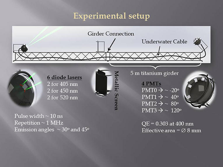
Figure 1. The experimental apparatus. Apart from the geometrical and construction characteristics of the apparatus, details of the light pulse and characteristics of the PMTs are also presented.

The experimentally measured and the simulated arrival time distributions were used to apply a χ² minimization process for the estimation of the aforementioned optical parameters. To overcome the high cost of the simulation process in resources and time, the minimization was based on a re-weighting method for the propagation in the parameters space [20]. This method relied on the fact that, given the recorded track history of a “detected” photon, a quantity proportional to the probability of a photon to follow the specific track as a function of the optical parameters can be calculated. This is illustrated in the following expression:

$\begin{array}{ll}P(L_a,L_s,p,a_{Rayl},a_{Mie})& \propto e^{-L/L_a}\times \left[{\displaystyle \underset{i=1}{\prod ^{N-1}}}\frac{1}{L_s}F(cos{\theta }_i;p,a_{Rayl},a_{Mie})\right]\\ & \times e^{-l_N/L_s}& (4)\end{array}$

where N is the number of consecutive linear photon track segments (l_i), thus $L=\sum _{i=1}^N{l}_i$ is the total photon track length. The right part of Equation (4) consists of three terms, where $e^{-L/L_a}$ is the probability for a photon not to be absorbed after traveling length L, $\underset{i=1}{\prod ^{N-1}}\frac{1}{L_s}F(cos{\theta }_i;p,a_{Rayl},a_{Mie})$ is proportional to the probability for a photon to be scattered with angle θ_i after having crossed a distance l_i, and $e^{-l_N/L_s}$ gives the probability for the photon not to be scattered at the last track segment until it reaches the detector.

To test the reliability of our method, a MC sample of events was produced, considered as the set of experimentally recorded events (hereafter pseudo-data), with parameters: L_a = 73m, L_s = 56.4m, p = 0.21, a_Mie = 0.75 and a second MC sample of events, considered as the simulated events, with parameters: L_a = 65m, L_s = 48.4m, p = 0.17, a_Mie = 0.924. In all samples of events a_Rayl was fixed to a_Rayl = 0.853, since it is a well-known factor, attributable to the anisotropy of water molecules [21], and additionally its variations have insignificant impact in the resulting arrival time distributions. Using the re-weighting technique of Equation (4), a χ² fit was applied of the simulated arrival time distributions to the corresponding ones from the pseudo-data and a set of estimated parameters was calculated. The minimization procedure was made in the five dimensional parameters space, where c was a normalization parameter related to the total number of generated photons. This method is insensitive to the absolute intensity of the light pulses. The crucial parameters contributing to the sensitivity of the method relies on the shape as well as the relative intensity of the different PMT signal time distributions. The “real” parameters were well estimated from the final fit with the following uncertainties: δp = 0.0019 (0.9%), δL_s = 1.34 m (2.4%), δL_a = 2.14 m (2.9%) and δa_Mie = 0.0023 (0.3%).

The experimental apparatus

Using the MC software described above, we studied the optimum geometrical parameters and the optimum signal characteristics of our experimental apparatus, assuming that the main background was due to the K40 activity, estimated to be < 100 Hz [22]. The experimental apparatus described below meets all the specified requirements.

Description of the apparatus

The experimental apparatus consisted of four, 5 m long titanium girders, attached to each other so that to form a linear and robust structure (Figure 1). One of the girders had a 17^′′ diameter glass sphere attached. Inside this glass sphere three pairs of laser diodes were placed, emitting at wavelengths 405, 450, and 520 nm. At the other end of the same girder a metallic screen was placed in order to avoid the exposure of the detectors to direct light. A second girder was equipped with a 17^′′ diameter glass sphere that housed the four, 8 mm diameter, HAMAMATSU H10682-210 photomultipliers (PMTs). Those two girders when connected to each other were forming the 10 m long configuration of the measurement apparatus. The other two girders carried no equipment and were connected to the two equipped ones, so that the 15 m and 20 m configurations were formed. The 15 m configuration was formed by connecting an unequipped girder between the two equipped ones at the Girder Connection point (see Figure 1). The 20 m configuration was similarly formed by adding the fourth unequipped girder in the 15 m configuration of the apparatus. In order to minimize unwanted light reflections, the girders, the metallic screen and all the supporting structure was painted with black matte paint. The two laser diodes in each pair were mounted inside the glass sphere with their axes forming an angle of 30° and 45° with respect to the axis connecting the centers of the glass spheres housing the lasers and the PMTs, respectively. The laser diodes emitted light pulses with pulse width ~10 ns at a repetition rate around of 1 MHz. On each laser diode a collimator was mounted on in order to achieve better focusing of the laser light. The four PMTs were placed in their glass sphere with their axes forming an angle of −20°, 40°, 80°, and 120° with respect to the axis formed by the centers of the glass spheres housing the lasers and the PMTs, respectively. The previously described configuration of the apparatus, with several lasers and PMTs placed at different angles and with different lengths of the apparatus, was chosen in order to cover with measurements a big part of the optical parameters space. The whole system was powered by, type VARTA D, batteries placed inside the lasers' and PMTs' glass spheres.

For electrically controlling the experimental apparatus an integration module based on a Xilinx Spartan-6 FPGA (type: XC6SLX16-2FTG256C) Opal Kelly XEM6001 board was used. It featured USB port for configuration downloads, and provided access to most of the Input/Output pins on the 256-pin Spartan 6 device. Also, a 32-bit AVR UC3 microcontroller was used (evaluation kit EVK1104). In addition to SD card, a High Speed USB2 port included for measured-data transferring. Finally, two custom made boards (PCBs) were built to enable power management and laser control features.

The design and functionality of the experimental apparatus's electronics is described in the block diagram of Figure 2. In this block diagram only the Laser Controller was implemented in the lasers' glass sphere, all the other components were implemented in the PMTs' glass sphere. The Laser Controller was responsible for driving the lasers with the proper electric pulse, so that a light pulse of < 10 ns duration and of energy < 2 pJ was produced. The Laser Controller was triggered by an electronic pulse produced by the Main Counter and sent to the Laser Controller via an underwater cable. The Main Counter was counting the 2.5 ns clock pulses and reset to 0 every 1,280 ns, synchronously with the Laser Controller trigger pulse. When a scattered photon hit one of the PMTs and an electronic pulse was produced, the PMT Controller (one PMT Controller per PMT) stored the current value of the Main Counter to a temporary register. The PMT Controller was capable of storing up to 3 pulses (scattered photons) for each laser pulse. Just before the Main Counter reset to 0, all temporary registers that have data were pushed to the FIFO, via the Mux and Gate Controller, together with a mask that defined the PMT which produced the data. In case the FIFO was full, the data of the current Main Counter cycle (current light pulse) were rejected. If the FIFO had enough space for the data to be stored, the Laser Pulse Counter was incremented. After 1,024 active light pulses the contents of the Laser Pulse Counter were stored to the FIFO via the Counter Controller, together with a mask that was recording the flushing laser as defined by the Microcontroller (M/C System). The selection of which laser to flush, was controlled by the Microcontroller together with the Time Controller which set (user selected) the time duration the laser would flush (this time was set to 30 s for the experiment). The Microcontroller was also controlling the power to the PMTs and enabling the FPGA. All data from the FIFO were finally stored to an SD-card attached to the Microcontroller, which was also handling the transfer of the data to the PC. The whole system (Lasers, PMTs, electronics) was powered from batteries placed in the PMTs' and lasers' glass spheres, as described above.

FIGURE 2

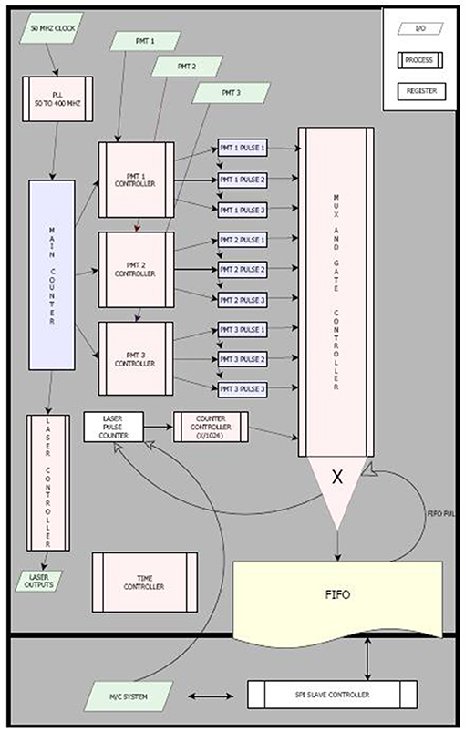
Figure 2. Block diagram of the electronics. The lasers' trigger, as well as, the PMTs' readout and data storage systems are graphically presented.

System measurements and tests

Before and after deployment an extensive series of tests and measurements of the experimental apparatus were performed. The most important of those are explained in the following paragraphs.

• Geometrical survey of the experimental apparatus: The lasers and the PMTs were mounted inside their glass spheres following a special mechanical procedure that guaranteed a positioning accuracy of better than 0.5 mm. This was furthermore confirmed by independently measuring the lasers' and PMTs' positions after construction. The PMTs' axis direction was estimated with an accuracy of < 1°, which was considered sufficient compared to the angular response specifications of the PMTs. The direction of the emitted laser light was determined with the help of a rigid screen placed at different distances (x) from the center of the lasers' glass sphere along and perpendicular to the titanium girder where the sphere was attached. Each laser diode was switched on and projected onto the screen. The spots centers where recorded, and the y and z coordinates for each distance × were determined. The measurement setup of the lasers' direction together with the corresponding coordinate system is shown in Figure 3. A line equation in a three dimensional space, representing a laser emission direction, was fitted to the data, and the emission directions in spherical coordinates were calculated with an accuracy of 0.2°.

• Using a laser distance meter, with a typical accuracy of ±1.5 mm, the distance between the centers of the lasers' and the PMTs' glass spheres was measured to be 935.6, 1445.7, and 1955.3 cm, for the three length configurations (10, 15, and 20m) of the apparatus, respectively. In the same way the distance between the metallic screen and the center of the lasers' glass sphere was found to be 424.8 cm.

• Laser pulse time distribution measurements: The laser pulse time distributions have been measured to be implemented in the generation of photons in the Monte Carlo simulation. To measure the time distributions, the data acquisition and driving electronics of the experiment were used. A PMT module was placed near the laser light sources and a 30 μm diameter pinhole was used to reduce the detected light flux suppressing the effect of the PMT's pulse-pair-resolution to the data. The lasers were flashing with a repetition rate of 781.25 kHz and the PMT hit arrival times were recorded in the 1,280 ns “time windows” (512 time-channels of 2.5 ns width) between the laser flashes. Due to the small distance of the PMT from the lasers and the high transparency of air for the laser wavelengths, the arrival and generation time distributions were practically the same. Assuming that the hit events in each time channel were distributed according to Poisson statistics the measured average hits per laser flash time distributions were further analyzed to correct the effect of the pulse-pair resolution (the pulse-pair resolution of the system was measured to be 35 ns). The resulting pulse distributions for the six lasers, as measured before deployment, are shown in Figure 4.

• Laser emission angle distribution measurements: The characterization of the laser emission angle distributions was performed by angular scanning with a custom made device that had been designed and constructed by the team. The properly calibrated system (shown in Figure 5) was driven by two step-motors, thus rotating the glass sphere around the two yellow axes. A PMT was placed in a fixed distance of x = 2 m from the center of the glass sphere with a 30 μm diameter pinhole, reducing its detection effective area. The photoelectron hit rate of the PMT was measured with a CNT-90 counter. The radiation flux at a direction (θ, ϕ) in spherical coordinates was measured by rotating the system by angles Φ1 and Φ2 around the two rotation axes, respectively. Dedicated software was developed to automate the scanning process giving as a result the angular hit rate “map” of the laser spots. The scan-data derived were cross-checked to the aforementioned measured laser directions (colored circles in Figure 6) giving a good fit. The pulse pair resolution of the PMT was also taken into account and the data were corrected accordingly.

• Underwater cable delay and voltage drop measurements: We studied the behavior of the underwater cable, through which the trigger signal was sent to the lasers from the Main Counter in the PMTs' glass sphere. A continuous square pulse of frequency 0.78 MHz and with amplitude limits set to 3.8 V high voltage and 1.2 V low voltage was generated by the Tektronix AFG 3252 Dual Channel function generator. The signal was guided to the underwater cable (37.5 m long) and the output of the signal was guided through a 50 Ohm resistance to the Lecroy WaveRunner oscilloscope. The delay of the signal on air was found to be 256 ns. The time delay of the pulse was measured under pressure up to 400 bars, with step of 50 bars. The results of our measurements are shown in Table 1. Alkaline batteries of type VARTA D (operating voltage of 1.6 V) were used for the autonomous supply of the experimental apparatus and the total amount of batteries had to be calculated. Six such batteries, connected in series were used, in order to supply our system. A blue laser was sending light to a PMT, at maximum intensity, resulting to a recording rate at the PMT exit (before the FPGA) of 1.34 MHz to 1.35 MHz. The voltage (V) and current (mA) at different times were measured. Our results are shown in Figure 7. The irregularity that was recorded at 7.3 V was due to the fact that the system was paused at that time and for some time no measurements were recorded. It is clear that the voltage was dropping while the current was increasing, resulting in an almost stable power that was consumed by the FPGA system (~2.3 mW). When the voltage was dropping below 6.5 V the system did not give reliable results (irregularities in current measurements and PMT rates were observed). We concluded that by filling the free space inside the glass spheres with batteries the system could be operated for more than 48 h continuously and with rather good stability. For longer operation we expect a deterioration of the apparatus' performance, due to the limited lifetime of the batteries.

• PMT dark rate measurements: The dark rate of the PMTs was measured as a function of time. The measured dark rates of all PMTs correspond to the specified values of the manufacturer (typical 50 Hz). After 1 h of measurements the dark rate of all PMTs fell below 10 Hz, to be compared with the ~100 Hz rate of the K40 background and the 10 kHz rate of the recorded scattered light, according to specifications. The temperature and humidity of the environment where the system was placed were, T = 24.5 °C and H = 23.58 %, respectively.

• Performance tests of the electronics: Using 10 ns width pulses from a pulse generator (Tektronix AFG 3252), to emulate the pulses produced by the PMTs, we were able to confirm that the whole electronics chain of the system was working according to its specifications and design. Namely, the recorded pulse rates measured were found to be within specifications (10 kHz), as well as the time resolution of the system was found to be 2.5 ns with very high accuracy. In addition, the system was found to be capable to record up to 3 pulses (scattered photons) per light pulse without any lose on the recorded pulse rates. By sending pairs of 10 ns pulses separated by a preset time difference the pulse-pair resolution of the system was found to be 35 ns.

• System stability tests: All the system tests described above were performed before and after deployment, so as to control the stability of the system. Unfortunately, a technical problem at the time of sealing the lasers' glass sphere caused the damage (significantly different time and intensity distributions of the emitted light) of both the 450 nm lasers, and of the 405 nm and 520 nm lasers pointing to the “45° direction” and “30° direction,” respectively. The remaining lasers (405 nm, “30° direction” and 520 nm, “45° direction”) demonstrated a rather good stability in the aforementioned tests and were used for analysis.

FIGURE 3

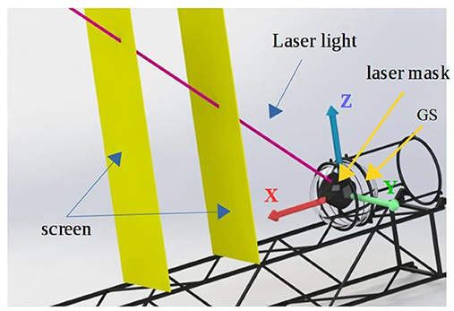
Figure 3. Setup and system of coordinates for the measurement of the laser directions. The lasers (laser mask) are placed inside the lasers' glass sphere (GS), in fixed positions (x, y, z) with respect to the center of the sphere.

FIGURE 4

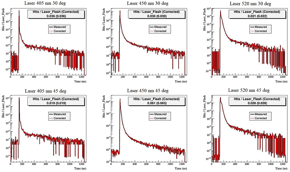
Figure 4. Pulse time distributions (hits per laser flash distribution as a function of time) for the six lasers, as measured before deployment.

TABLE 1

Table 1. Cable delay as a function of pressure.

FIGURE 5

Figure 5. 3D graphical representation of the angular scanning system. The properly calibrated system was driven by two step-motors, thus rotating the glass sphere around the two yellow axes.

FIGURE 6

Figure 6. θ-ϕ mapping of the lasers' spot. The scan-data derived were cross-checked to the measured laser directions (colored circles).

FIGURE 7

Figure 7. Batteries' voltage (V) drop and current (mA) passing through the measuring system at different times.

Measurement details and analysis

The site chosen for the deployment of the detector was the western side of Pylos (360 31′ B and 210 26′ A), 40 km from shore at a sea depth of ~4,500 m. On October 28, 2015 the R/V “Aegeon” ship of the Hellenic Center for Marine Research was used in order to perform the deployment of the experimental apparatus. Three deployments of the apparatus were attempted, one for each of the three distance configurations of our system, i.e., 10, 15, and 20 m, respectively. In each deployment the apparatus was taking data for 1 h in total, at a depth of ~3,500 m. Three data sets were taken, one for each of the three deployments of the apparatus. Each data-set contains information about the arrival time distributions of the photons detected at the four PMT modules, for each of the six laser diodes. This means that from each dataset 24 histograms of arrival time distributions are extracted, giving an overall of 72 histograms for the experiment. Unfortunately, the aforementioned technical problem left only the 405 and 520 nm data for analysis. These distributions contain the desired absorption and scattering information to be extracted at the analysis–reconstruction process. Life activity in the deep sea water has been also observed from the analysis of the data. Figure 8 represents part of the “history” of the measurement at the second deployment (15 m configuration) as recorded from one of the four PMTs. Bioluminescence is observed by a temporary uniform increase of the detected photon rate inside the 1,280 ns “time window,” lasting less than a few seconds. Shadowing effects were also observed, most probably originating from live activity in the sea water. All data were processed before analysis, so to remove all the bioluminescence background and shadowing effects. In Figure 8, all the lasers are shown, not only the ones used in the analysis. As mentioned above the lasers that were not used in the analysis demonstrated instability on their pulse time and laser direction measurements before and after deployment.

FIGURE 8

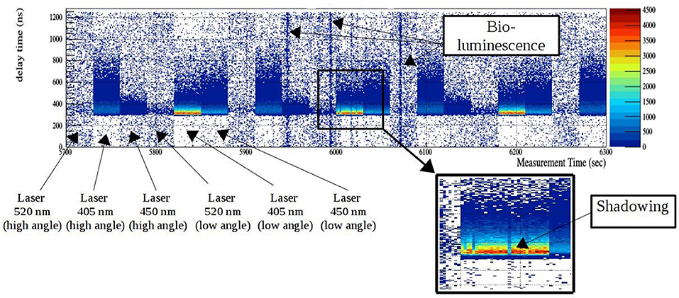
Figure 8. Part (600 sec) of the “measurement history” as recorded from one of the PMTs at the second deployment. In x is the real time of the measurement in seconds; in y are the time channels in the 1,280 ns “time window” and in z the hit rate in Hz for each measurement second at each time channel. The 30 s operation cycles of each laser as well as bioluminescence and shadowing effects can be observed.

Results

The time distributions of the signals, in the four photomultipliers for the three distances from the light sources (three deployments) and for the two diode lasers (405 and 520 nm) were derived from the analysis of the experimental data. The experiment was simulated, considering the geometry and the materials of the experimental setup, as well as the characteristics of the used PMTs and the lasers, as measured in the laboratory and explained in detail in section The Experimental Apparatus. A very large number of photons were generated for each laser. The propagation of the generated photon in the medium surrounding the setup, governed by the theoretical model described in section Description of the Method, was simulated with the help of GEANT Monte Carlo simulation packages. The optical parameters used for the simulation where those of section Parameters Estimation Method for the simulated sample of events (not the pseudo-data). The PMT signals derived from the simulation were fitted to the experimental ones by the implementation of the “re-weighting” method, described in section Parameters Estimation Method. For the fitting process, the ROOT–MINUIT package was used. Figures 9, 10 are representative plots of the fitting procedure. The dots in the plots of Figure 9 represent the experimental data in photons per laser pulse, for the “30° direction”- 405 nm laser. The data presented were recorded by the PMT at 40° direction in the 10 m (upper histogram) and 15 m (lower histogram) configurations. The red line represents the, fitted to the experimental data, theoretical model (simulation). Figure 10 shows the corresponding results for the “45° direction”-520 nm laser. The data presented were recorded by the PMT at 120° direction in the 10 m (upper histogram) and 15 m (lower histogram) configurations. The results of the fit to the experimental data are summarized in Table 2, together with the parameters' statistical errors as calculated from the fit.

FIGURE 9

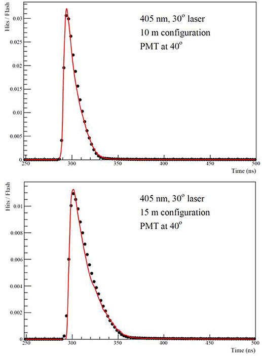
Figure 9. Photons per laser pulse for the “30° direction,” 405 nm laser (dots with statistical errors presented by the size of the dot). The data presented were recorded by the PMT at 40° direction in the 10 m (upper histogram) and 15 m (lower histogram) configurations The red line represents the, fitted to the experimental data, theoretical model (simulation).

FIGURE 10

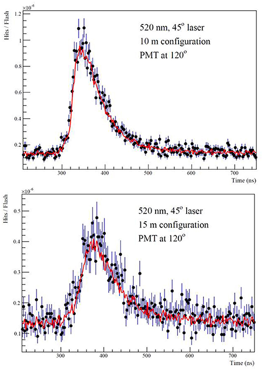
Figure 10. Photons per laser pulse for the “45° direction,” 520 nm laser (dots with statistical errors). The data presented were recorded by the PMT at 120° direction in the 10 m (upper histogram) and 15 m (lower histogram) configurations The red line represents the, fitted to the experimental data, theoretical model (simulation).

TABLE 2

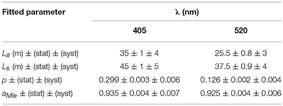
Table 2. Fit results with statistical and systematic errors (1σ).

The measurements and tests of the apparatus, as discussed in section System Measurements and Tests, cover all possible sources of systematic uncertainties. Each systematic error was calculated independently using the fitting procedure described above. All systematic errors were added in quadrature and the total effect of the systematic uncertainties is summarized in Table 2. The uncertainties in the laser emission angle and the pulse time distributions were dominating the systematic errors. In Figure 9 most of the data points in the decay curve are above the fitting curves. This small shift can be explained by the increased sensitivity of the fitting method to the time measurements, compared to the accuracy (~2 ns) the time was measured in the experiment and during the “Laser pulse time distribution” and “Underwater cable delay” measurements (see section System Measurements and Tests). In Figure 11 all time-measurements of the relevant PMT were shifted by 0.7 nm and the data were refitted. The results of this fit agree, within systematic errors, with the results of the fit presented in Table 2.

FIGURE 11

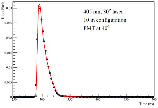
Figure 11. Photons per laser pulse for the “30° direction,” 405 nm laser (dots with statistical errors presented by the size of the dot). The data presented were recorded by the PMT at 40° direction in the 10 m configuration, after correcting the measured times by 0.7 ns.

Discussion

The photon propagation parameters in the sea water have been studied by several experiments in the past. Most of them focused on measuring the transparency of sea water [23–28). The most recent measurement was published by Anasontzis et al. [29), reporting a transmission length of ~26 m for λ = 400 nm and ~21 m for λ = 520 nm emission at a depth of 3,400 m.

The absorption and scattering properties of the sea water [21) for λ = 473 nm and λ = 375 nm have been measured by the ANTARES collaboration. In this experiment, the distribution of the arrival times of photons emitted by a pulsed LED source was recorded and collected several tens of meters away (24 m and 44 m) by a fast photomultiplier tube. Both direct and scattered light were recorded since no screening technique has been used. A wide variety of measurements of the absorption length has been taken, depending on the epoch, in the range between 49 and 69 m for wavelength of 473 nm and between 24 and 29 m for 375 nm. The corresponding ranges for the scattering length were 38 to 62 m for λ = 473 nm and 24–28 m for the λ = 375 nm.

In this measurement direct light is blocked, thus leaving scattered only photons to be recorded by the apparatus and enhancing the sensitivity of our measurements on the scattering parameters of the light propagation in the sea water. Furthermore, the combination of different lasers' and PMTs' orientations and of different lengths of the apparatus, results on a much wider coverage of the optical parameters' space with measurements, thus allowing a more detailed and accurate study of the optical parameters of the sea water. Unfortunately, the technical problem appeared at the time of sealing the lasers' glass sphere has resulted on bigger statistical and systematic errors than has originally been anticipated. As a result our measurements were restricted in only two wavelengths. Nevertheless, the presented results are in a satisfactory agreement with previous measurements and prove that such an apparatus can be used for the in situ measurement of the instantaneous values of all relevant parameters of the light propagation in the sea water.

Author contributions

MM: Electronics engineer contributed on the design and development of the apparatus's electronics. All other authors contributed on the construction of the apparatus and on data taking and analysis.

Funding

This Research has been funded by the Greek General Secretariat for Research & Technology within the framework of the Action entitled ≪Proposals for Development of Research Bodies-KRIPIS≫-NSRF (Operational Program II, Competitiveness & Entrepreneurship).

Conflict of interest statement

The authors declare that the research was conducted in the absence of any commercial or financial relationships that could be construed as a potential conflict of interest.

Acknowledgments

We thank our electronics and machine shop teams, especially I. Kiskiras for his continuous supportive work on the project. We also thank the Captain, Officers and Crew of the R/V Aegeon.

References

1. Formaggio JA, Zeller GP. From eV to EeV: Neutrino cross sections across energy scales. Rev Mod Phys. (2012) 84:1307. doi: 10.1103/RevModPhys.84.1307

CrossRef Full Text | Google Scholar

2. Gandhi R, Quigg C, Reno MH, Sarcevic I. Ultrahigh-energy neutrino interactions. Astropart Phys. (1996) 5:81–110. doi: 10.1016/0927-6505(96)00008-4

CrossRef Full Text | Google Scholar

3. Connolly A, Thorne RS, Waters D. Calculation of high energy neutrino-nucleon cross sections and uncertainties using the MSTW Parton distribution functions and implications for future experiments. Phys Rev D (2011) 83:113009. doi: 10.1103/PhysRevD.83.113009

CrossRef Full Text | Google Scholar

4. Balasi KG, Langanke K, Martinez-Pinedo G. Neutrino-nucleus reactions and their role for supernova dynamics and nucleosynthesis. Prog Part Nucl Phys. (2015) 85:33–81. doi: 10.1016/j.ppnp.2015.08.001

CrossRef Full Text | Google Scholar

5. Ydrefords E, Balasi KG, Kosmas TS, Suhonen J. The response of 95, 97Mo to supernova neutrinos. Nucl Phys A (2011) 866:67–78. doi: 10.1016/j.nuclphysa.2011.07.007

CrossRef Full Text | Google Scholar

6. Ydrefors E, Balasi KG, Kosmas TS, Suhonen J. Detailed study of the neutral-current neutri-no–nucleus scattering off the stable Mo isotopes. Nucl Phys A (2012) 896:1–23. doi: 10.1016/j.nuclphysa.2012.10.001

CrossRef Full Text | Google Scholar

7. Klein SR. Muon production in relativistic cosmic-ray interactions. Nucl Phys. (2009) A830:869c–72c.

Google Scholar

8. Pasquali L, Reno M, Sarcevic I. Lepton fluxes from atmospheric charm. Phys Rev D (1999) 59:034020.

Google Scholar

9. Abbasi R, Abdou Y, Abu-Zayyad T, Adams J, Aguilar JA, Ahlers M, et al. Search for dark matter from the Galactic halo with the icecube neutrino telescope. Phys Rev D (2011) 84:022004. doi: 10.1103/PhysRevD.84.022004

CrossRef Full Text | Google Scholar

10. Čerenkov PA. Visible radiation produced by electrons moving in a medium with velocities exceeding that of light. Phys Rev. (1934) 52:378. doi: 10.1103/PhysRev.52.378

CrossRef Full Text | Google Scholar

11. Jackson JD. Classical Electrodynamics, 3rd ed. Hoboken, NJ: John Wiley and Sons Inc , (1998).

Google Scholar

12. C.F. Bohren, D. Huffman. Absorption and Scattering of Light by Small Particles. New York, NY: John Wiley (1983).

13. Adrián-Martínez S, Ageron M, Aharonian F, Aiello S, Albert A, Ameli F, et al. Deep sea tests of a prototype of the KM3NeT digital optical module: KM3NeT collaboration. Eur Phys J C (2014) 74:3056. doi: 10.1140/epjc/s10052-014-3056-3

CrossRef Full Text | Google Scholar

14. Adrian-Martinez S, Ageron M, Aharonian F, Aiello S, Albert A, Ameli F, et al. The prototype detection unit of the KM3NeT detector. Eur. Phys. J. C (2015) 76:54. doi: 10.1140/epjc/s10052-015-3868-9

CrossRef Full Text | Google Scholar

15. Maragos N, Balasi K, Domvoglou T, Kiskiras I, Lenis D, Maniatis M, et al. Measurement of light scattering in deep sea. EPJ Web Conf. (2016) 116:06009. doi: 10.1051/epjconf/201611606009

CrossRef Full Text | Google Scholar

16. Balasi KG, Domvoglou T, Kiskiras I, Lenis D, Maniatis M, Maragos N, et al. An autonomous underwater telescope for measuring the scattering of light in the deep sea. J Phys Conf Ser. (2016) 718:062002. doi: 10.1088/1742-6596/718/6/062002

CrossRef Full Text | Google Scholar

17. Lockwood DJ. Rayleigh and mie scattering. In: Luo MR. editor. Encyclopedia of Color Science and Technology. New York, NY: Springer (2015).

Google Scholar

18. Toublanc D. Heney-Greenstein and Mie phase functions in Monte Carlo radiative transfer computations. Appl Opt. (1996) 35:3270–4. doi: 10.1364/AO.35.003270

CrossRef Full Text | Google Scholar

19. Amako K, Guatelli S, Ivanchencko V, Maire M, Mascialino B, Murakami K Geant4 and its validation. Nuclear Phys B (2006) 150:44–49. doi: 10.1016/j.nuclphysbps.2004.10.083

CrossRef Full Text | Google Scholar

20. Papaoikonomou A, Leisos Tsirigotis A, Tzamarias S. A Technique for Measuring the Sea Water Optical Parameters with a Dedicated Laser Beam and a Multi-PMT Optical Module. Stockholm: Workshop on very large volume neutrino telescopes (2013)

Google Scholar

21. The ANTARES Collaboration Aguilar JA, Albert A, Amram P, Anghinolfi M, Anton G, et al. Transmission of light in deep sea water at the site of the ANTARES neutrino telescope. Astroparticle Phys. (2005) 23:131–55. doi: 10.1016/j.astropartphys.2004.11.006

CrossRef Full Text | Google Scholar

22. Löhner H, Dorosti-Hasankiadeh Q, Heine E, Gajanana D, Kavatsyuk O, Kooijman P, et al. The multi-PMT optical module for KM3NeT. In: Proceedings of the 12th Pisa Meeting on Advanced Detectors: La Biodola, Isola d'Elba (2012).

Google Scholar

23. Zaneveld JRV. Proceedings of the 1980 International DUMAND Symposium. Honolulu: V. J. Stenger (1981), 1–8.

Google Scholar

24. Belolaptikov IA, Bezrukov LB, Borisovets BA, Budnev NM, Chensky AG, Djilkibaev ZhAM, et al. The lake Baikal underwater telescope NT-36: first months of operation. Nucl Phys Proc Suppl. (1994) 35:290–3. doi: 10.1016/0920-5632(94)90266-6

CrossRef Full Text | Google Scholar

25. Cuickenden TI, Irvin JA. The ultraviolet absorption spectrum of liquid water. J Chem Phys. (1980) 72:441. doi: 10.1063/1.439733

CrossRef Full Text | Google Scholar

26. Boivin LP, Davidson WF, Storey RS, Sinclair D, Earle ED. Determination of the attenuation coefficients of visible and ultraviolet radiation in heavy water. Appl Opt. (1986) 25:877–82.

PubMed Abstract | Google Scholar

27. Sogandares FM, Fry S. Absorption spectrum (340–640 nm) of pure water. I. Photothermal measurements. Appl Opt. (1997) 36:8699–709.

PubMed Abstract | Google Scholar

28. Pope RM, Fry ES. Absorption spectrum (380–700 nm) of pure water. II. Integrating cavity measurements. Appl. Opt. (1997) 36:8710–23.

PubMed Abstract | Google Scholar

29. Anassontzis EG, Ball AE, Belias A, Fotiou A, Grammatikakis G, Kontogiannis H, et al. Water transparency measurements in the deep Ionian Sea. Astropart Phys. (2010) 34:187–97. doi: 10.1016/j.astropartphys.2010.06.008

CrossRef Full Text | Google Scholar