Dark Matter With Stückelberg Axions

1. Introduction

It is by now well established that astrophysical and cosmological data coming either from measurements of the velocities of stars orbiting galaxies, in their rotation curves, or from the cosmic microwave background, indicate that about ~80% of matter in the universe is in an unknown form, and the expectations for providing an answer to such a pressing question run high. These observational results are justified within the standard ΛCDM dark matter/dark energy model [1] which has been very successful in explaining the data. It predicts a dark energy component about 68 ± 1% of the total mass/density contributions of our universe in the form of a cosmological constant. The latter accounts for the dark energy dominance in the cosmological expansion at late times and provides the cosmological acceleration measured by Type Ia supernovae [2, 3], with ordinary baryonic dark matter contributing just a few percent of the total mass/energy content (~5%) and a smaller neutrino component. Cold dark matter with small density fluctuations, growing gravitationally and a spectral index of the perturbations n_S ~ 1 is compatible with an early inflationary stage and accounts for structure formation in most of the early universe eras. By now, data on the CMB, weak lensing and structure formation, covering redshifts from large z ~ 10³ down to z <~ O(1) where the full nonlinear regime of matter dominance is at work, have been confronted with N-body gravitational simulations for quite some time, with comparisons which are in general agreement with ΛCDM. Such simulations, characterized by perturbations with the above value of the spectral index show the emergence of hierarchical, self-similar structures in the form of halos and sub-halos of singular density (ρ(r) ~ 1/r in terms of the radius r) [4] in the nonlinear regime. However, while the agreement between ΛCDM and the observations is significant at most scales, at a small sub-galactic scale, corresponding to astrophysical distances relevant for the description of the stellar distributions (~10 kpc), cold dark matter models predict an abundance of low-mass halos in excess of observations [5]. Difficulties in characterizing this sub-galactic region have usually been attributed to inaccurate modeling of its baryonic content, connected with star formation, supernova explosions and black hole activity which take place in that region, causing a redistribution of matter.

There are various possibilities to solve this discrepancy, such as invoking the presence of warm dark matter (WDM), whose free streaming, especially for low mass WDM particles, could erase halos and sub-halos of low mass. At the same time, they could remove the predicted dark matter cusps in ρ(r), present in the simulations for r ≃ 0 [4] but are not detected observationally. As observed in Hu et al. [5] and recently re-addressed in Hui et al. [6], these issues define a problem whose resolution may require a cold dark matter component which is ultralight, in the 10⁻²⁰ − 10⁻²² eV range. Proposals for such a component of dark matter, find motivations mostly within string theory, where massless moduli in the form of scalar and pseudoscalar fields abound at low energy. They are introduced at the Planck scale and their flat potentials can be lifted by a small amount, giving rise to ultralight particles. However, the characterization of a well-defined gauge structure which may account for the generation Of such ultralight particle(s) and which may eventually connect the speculative scenarios to the electroweak scale, can be pursued in various ways. It has recently been proposed [7] that particles of this kind may emerge from a grand unification in the presence of anomalous abelian symmetries, revisiting previous constructions.

The goal of this review is to summarize the gauge structure of these models which require an anomalous fermion spectrum with gauge invariance restored by a Wess-Zumino interaction, by the inclusion of a Stückelberg axion. Such models can be thought as the field theory realization of the mechanism of anomaly cancellation derived from string theory. The models reviewed here are characterized by some distinctive key features that we discuss, in order to establish their relation to the Peccei-Quinn model, of which they are an extension at a field theory level.

2. Anomalous U(1)′s

The Peccei-Quinn (PQ) mechanism, proposed in the 1970's to solve the strong CP problem [8–10], had originally been realized by assigning an additional abelian chiral charge to the fermion spectrum of the Standard Model (SM). Alternatively, a similar symmetry can be present in a natural way in specific gauge theories based on groups of higher ranks with respect to the SM gauge group. This is the case, for instance of the U(1)_PQ symmetry found in the E₆ GUT discussed in Frampton and Kephart [11] (as well as in other realizations), which is naturally present in this theory and which can lead to a solution of the strong CP problem.

As we are going to discuss, the mass of the axion, either in the presence of global or local anomalies is connected to the instanton sector of a non-abelian theory and it is crucial for the mechanism of misalignment to be effective so that the axion couples to the gauge sector of the same theory. In fact, the possibility that more than one axion is part of the spectrum of a certain gauge theory is not excluded, with the mass of each axion controlled by independent mechanism(s) of vacuum misalignment induced at several scales, if distinct gauge couplings for each of such particles with different gauge sectors are present [12, 13]. We will illustrate this point in the extended E₆ theory, in the next sections, where the inclusion of an extra anomalous U(1) gauge symmetry realizes such a scenario. Different mechanisms of vacuum misalignment may be responsible for the generation of axions of different masses, whose sizes may vary considerably.

2.1. Anomaly Cancellation at Field Theory Level With an Axion

In the case of a Stückelberg axion, as already mentioned, the PQ symmetry is generalized from a global to a local gauge symmetry and the Wess-Zumino interactions are needed for the restoration of gauge invariance of the effective action. Such generalizations, originally discussed in the context of low scale orientifold models [14], where anomalous abelian symmetries emerge from stacks of intersecting branes, have in the past been proposed as possible scenarios to be investigated at the LHC [15–20], together with their supersymmetric extensions [13, 21, 22]. While anomalous abelian symmetries are interesting in their own right, especially in the search for extra neutral currents at the LHC [18, 23–25], one of the most significant aspects of such anomalous extensions is in fact the presence of an axion which is needed in order to restore the gauge invariance of the effective action. It was called the “axi-Higgs” in Corianò et al. [14] and Corianò and Irges [15]–for being generated by the mechanism of Higgs-Stückelberg mixing in the CP-odd scalar sector, induced by a PQ-breaking periodic potential, later studied for its implications for dark matter in Corianò et al. [12]. The appearance of such a potential is what allows one component of the Stückelberg field to become physical. A periodic potential can be quickly recognized as being of instanton origin and related to the θ-vacuum of Yang-Mills theory and can be associated with phase transitions in non-abelian theories. Recent developments have considered the possibility that the origin of such a potential of this form can be set at a very large scale, such as the scale of grand unification (GUT). Its size is related to the value of the gauge coupling at the GUT scale, characterized by a typical instanton suppression, where the mechanism of vacuum misalignment takes place.

2.2. An Ultralight Axion

In the case of a misalignment generated at the GUT scale, the mass of the corresponding axion is strongly suppressed and can reach the far infrared, in the range of 10⁻²⁰ − 10⁻²² eV, which is in the optimal range for a possible resolution of several astrophysical issues, such as those mentioned in the introduction [6]. Proposals for a fuzzy component of dark matter require a weakly interacting particle in that mass range. As in the PQ (invisible axion) case. Additionally, in this case two scales are also needed in order to realize a similar scenario. In the PQ case the two scales correspond to f_a, the large PQ breaking scale and the hadronic scale which links the axion mass, f_a, the pion m_π and the light quarks masses m_u, m_d, in an expression that we will summarize below. In the case of Stückelberg axions these fields can be introduced as duals of a 2-form (B_μν), defined at the Planck scale (M_P) and coupled to the field strength (F) of an anomalous gauge boson via a B ∧ F interaction [7].

The mechanism of Higgs-axion mixing and the generation of the periodic potential can take place at a typical GUT scale. It is precisely the size of the potential at the GUT scale, which is controlled by the θ-vacuum of the corresponding GUT symmetry, which is responsible for the generation of an ultralight axion in the spectrum. As already mentioned, in the model discussed in Corianò and Frampton [7] a second axion is present, specific to the E₆ part of the E₆ × U(1)_X symmetry, which is sensitive to the SU(3) color sector of the Standard Model after spontaneous symmetry breaking. This second field takes the role of an ordinary PQ axion and solves the strong CP problem. We will start by recalling the main features of the PQ solution, in particular the emergence of a mass/coupling relation in such a scenario which narrows the window for axion detection down and gets enlarged in the presence of a gauge anomaly in Stückelberg models [20]. We will then turn, in the second part of this review, to a discussion of the Stückelberg extension. We will describe the features of such models in them non-supersymmetric formulation. Their supersymmetric version requires a separate discussion, for predicting both an axion and a neutralino as possible dark matter relics [13, 22].

3. The Invisible PQ Axion

The theoretical prediction for the mass range in which to locate a PQ axion is currently below the eV region. The PQ solution to the strong CP problem has been formulated according to two main scenarios involving a light pseudoscalar (a(x)) which nowadays take the name from the initials of the proponents, the KSVZ axion (or hadronic axion) and the DFSZ [26, 27] axion, the latter introduced in a model which requires, in addition, a scalar sector with two Higgs doublets H_u and H_d, besides the PQ complex scalar Φ.

The small axion mass is attributed to a vacuum misalignment mechanism generated by the structure of the QCD vacuum at the QCD phase transition, which causes a tilt in the otherwise flat PQ potential. The latter undergoes a symmetry breaking at a scale v_PQ, in general assumed to lay above the scales of inflation H_I and of reheating (T_R), and hence quite remote from the electroweak/confinement scales. Other possible locations of v_PQ with respect to H_I and T_R are also possible.

In both solutions the Peccei-Quinn scalar field Φ, displays an original symmetry which can be broken by gravitational effects, with a physical Goldstone mode a(x) which remains as such from the large v_PQ scale down to Λ_QCD, when axion oscillations occur. In the DFSZ solution, the axion emerges as a linear combination of the phases of the CP-odd sector and of Φ which are orthogonal to the hypercharge (Y) and are fixed by the normalization of the kinetic term of the axion field a. The solution to the strong CP problem is then achieved by rendering the parameter of the θ-vacuum dynamical, with the angle θ replaced by the axion field (θ → a/f_a), with f_a being the axion decay constant. The computation of the axion mass m_a is then derived from the vacuum energy of the θ-vacuum E(θ) once this is re-expressed in terms of the QCD chiral Lagrangian, which in the two quark flavor (u,d) case describes the spontaneous breaking of the SU(2)_L × SU(2)_R flavor symmetry to a diagonal SU(2) subgroup, with the 3 Goldstone modes (π^±, π⁰) being the dynamical field of the low energy dynamics. In this effective chiral description in which the θ parameter is present, the vacuum energy acquires a dependence both on neutral pseudoscalar π⁰ and on θ of the form

$\begin{array}{ll}E({\pi }^0,\theta )=-m_{\pi }^2{f}_{\pi }^2\sqrt{{cos}^2\frac{\theta }{2}+{\left(\frac{m_d-m_u}{m_d+m_u}\right)}^2{sin}^2\frac{\theta }{2}}cos\left({\pi }^0-\varphi (\theta )\right)& (1)\end{array}$

with

$\begin{array}{ll}\varphi (\theta )\equiv \frac{m_d-m_u}{m_d+m_u}sin\frac{\theta }{2}.& (2)\end{array}$

At the minimum, when ${\pi }^0=f_{\pi }\varphi (\theta )$, the vacuum energy assumes the simpler form

$\begin{array}{ll}E(\theta )=-m_{\pi }^2{f}_{\pi }^2\sqrt{1-\frac{4m_u{m}_d}{{(m_u+m_d)}^2}{sin}^2\frac{\theta }{2}}& (3)\end{array}$

which expanded for small θ gives the well-known relation

$\begin{array}{ll}E(\theta )=-m_{\pi }^2{f}_{\pi }^2+\frac{1}{2}{m}_{\pi }^2{f}_{\pi }^2\frac{m_u{m}_d}{{(m_u+m_d)}^2}{\theta }^2+\dots & (4)\end{array}$

and the corresponding axion mass

$\begin{array}{ll}{m}_a^2=\frac{m_{\pi }^2{f}_{\pi }^2}{f_a^2}\frac{m_u{m}_d}{{(m_u+m_d)}^2}& (5)\end{array}$

as θ → a/f_a. Before getting into a more detailed analysis of the various possible extensions of the traditional PQ scenarios, we briefly review the KSVZ (hadronic) and DFSZ (invisible) axion solutions.

3.1. KSVZ and DFSZ Axions

In both the DFSZ and KSVZ scenarios a global anomalous U(1)_PQ symmetry gets broken at some large scale v_PQ, with the generation of a Nambu-Goldstone mode from the CP-odd scalar sector. In the KSVZ case the theory includes a heavy quark Q which acquires a large mass by a Yukawa coupling with the scalar Φ. In this case the Lagrangian of Q takes the form

$\begin{array}{ll}{L}=|\partial \text{Φ}{|}^2+i\bar{Q}\cancel{D}Q+\text{λΦ}{\bar{Q}}_L{Q}_R+h.c.-V(\text{Φ})& (6)\end{array}$

with a global U(1)_PQ chiral symmetry of the form

$\begin{array}{l}\text{Φ}\to e^{i\alpha }\text{Φ}\\ Q\to e^{-\frac{i}{2}\alpha {\gamma }_5}Q& (7)\end{array}$

with an SU(3)_c covariant derivative (D) containing the QCD color charge of the heavy fermion Q. The scalar PQ potential can be taken from the usual Mexican-hat form and it is U(1)_PQ symmetric. Parameterising the PQ field with respect to its broken vacuum

$\begin{array}{ll}\text{Φ}=\frac{\varphi +v_{pq}}{\sqrt{2}}{e}^{i\frac{a(x)}{v_{PQ}}}+\dots & (8)\end{array}$

the Yukawa coupling of the heavy quark Q to the CP-odd phase of Φ, a(x), takes the form

$\begin{array}{ll}\text{λ}\frac{v_{pq}}{\sqrt{2}}{e}^{i\frac{a(x)}{v_{PQ}}}{\bar{Q}}_L{Q}_R.& (9)\end{array}$

At this stage one assumes that there is a decoupling of the heavy quark from the low energy spectrum by assuming that v_PQ is very large. The standard procedure in order to extract the low energy interaction of the axion field is to first redefine the field Q on order to remove the exponential with the axion in the Yukawa coupling

$\begin{array}{cc}{e}^{i{\gamma }_5\frac{a\left(x\right)}{2vPQ}}{Q}_{L/R}\equiv Q_{L/R}^{\prime }.& (10)\end{array}$

This amounts to a chiral transformation which leaves the fermionic measure non-invariant

$\begin{array}{ll}\mathrm{\text{D}}\bar{Q}\mathrm{\text{D}}Q\to e^{i\int d^{4}x\frac{6a(x)}{32{\pi }^2{v}_{PQ}}G(x)\tilde{G}(x)}\mathrm{\text{D}}\bar{Q}\mathrm{\text{D}}Q& (11)\end{array}$

and generates a direct coupling of the axion to the anomaly $G\tilde{G}$. Here the factor of 6 is related to the number of L/R components being rotated, which is 6 if Q is assigned to the triplet of SU(3)_c.

The kinetic term of Q is not invariant under this field redefinition and generates a derivative coupling of a(x) to the axial vector current of Q. For n_f triplets, for instance, the effective action of the axion, up to dimension-5 takes the form

$\begin{array}{ll}{{L}}_{eff}=\frac{1}{2}{\partial }_{\mu }a(x){\partial }^{\mu }a(x)+\frac{6n_f}{32{\pi }^2{v}_{PQ}}a(x)G\tilde{G}+\frac{1}{v_{PQ}}{\partial }_{\mu }a\bar{Q}{\gamma }^{\mu }{\gamma }_{5}Q+\dots & (12)\end{array}$

where we have neglected extra higher dimensional contributions, suppressed by v_PQ.

In the case of the DFSZ axion, the solution to the strong CP problem is found by introducing a scalar Φ together with two Higgs doublets H_u and H_d. In this case one writes down a general potential, function of these three fields, which is SU(2) × U(1) invariant and possesses a global symmetry

$\begin{array}{ll}{H}_u\to e^{i\alpha X_u}{H}_u,H_d\to e^{i\alpha X_d}{H}_d,\text{ Φ}\to e^{i\alpha X_{\text{Φ}}}\text{Φ}& (13)\end{array}$

with X_u + X_d = − 2X_Φ. It is given by a combination of terms of the form

$\begin{array}{ll}V=V({{|H}_u|}^2,{|H_d|}^2,|\text{Φ}{|}^2,{|H_u{H}_d^{†}|}^2,{|H_u·H_d|}^2,H_u·H_d,{\text{Φ}}^2)& (14)\end{array}$

where H_u · H_d denotes the SU(2) invariant scalar product. The identification of the axion field is made by looking for a linear combination of the phases which is not absorbed by a gauge transformation. This can be done, for instance, by going to the unitary gauge and removing all the NG modes of the broken gauge symmetry. The corresponding phase, which is the candidate axion, is the result of a process of mixing the PQ field with the Higgs sector at a scale where the symmetry of the potential is spontaneously broken by the two Higgs fields.

4. TeV Scale: Stückelberg Axions in Anomalous U(1) Extensions of the Standard Model

Intersecting D-brane models are one of those constructions where generalized axions appear [28–31]. In the case in which several stacks of such branes are introduced, each stack being the domain in which fields with the gauge symmetry U(N) live, several intersecting stacks generate, at their common intersections, fields with the quantum numbers of all the unitary gauge groups of the construction, such as

$\begin{array}{c}U(N_1)\times U(N_2)\times \dots \times U(N_k)=SU(N_1)\times U(1)\times SU(N_2)\\ \times U(1)\times \dots \times SU(N_k)\times U(1).& (15)\end{array}$

The phases of the extra U(1)'s are rearranged in terms of an anomaly-free generator, corresponding to an (anomaly free) hypercharge U(1) (or U(1)_Y), times extra U(1)'s which are anomalous, carrying both their own anomalies and the mixed anomalies with all the gauge factors of the Standard Model. This general construction can be made phenomenologically interesting.

Using this approach, the Standard Model can be obtained by taking for example 3 stacks of branes: a first stack of 3 branes, yielding a U(3) gauge symmetry, a second stack of 2 branes, yielding a symmetry U(2) and an extra single U(1) brane, giving a gauge structure of the form SU(3) × SU(2) × U(1) × U(1) × U(1). Linear combinations of the generators of the three U(1)'s allow us to rewrite the entire abelian symmetry in the form $U{(1)}_Y\times U{(1)}^{\prime }\times U{(1)}^{″}$, with the remaining U(1)′ × U(1)″ factors carrying anomalies which need to be canceled by extra operators. The simplest realization of the Standard Models (SM) is obtained by 2 stacks and a single brane at their intersections, giving a symmetry U(3) × U(2) × U(1). In this case, in the hypercharge basis, the gauge structure of the model can be rewritten in the form $SU{(3)}_c\times SU{(2)}_w\times U{(1)}_Y\times U{(1)}^{\prime }\times U{(1)}^{″}$.

We consider the case of a single $U{(1)}^{\prime }\equiv U{(1)}_B$ anomalous gauge symmetry, where the Stückelberg field b(x) couples to the gauge field B_μ by the gauge invariant term

$\begin{array}{ll}{{L}}_{St}=\frac{1}{2}{\left({\partial }_{\mu }b-M{B}_{\mu }\right)}^2& (16)\end{array}$

which is the well-known Stückelberg form. M is the Stückelberg mass. The Stückelberg symmetry of the Lagrangian (16) is revealed by acting with gauge transformations of the gauge fields B_μ under which the axion b varies by a local shift

$\begin{array}{ll}{\delta }_B{B}_{\mu }={\partial }_{\mu }{\theta }_B\delta b=M{\theta }_B& (17)\end{array}$

parameterized by the local gauge parameters θ_B. Originally, the Stückelberg symmetry was presented as a way to give a mass to an abelian gauge field while still preserving the gauge invariance of the theory. However, it is clear nowadays that its realization is the same one as obtained, for instance, in an abelian-Higgs model when one decouples the radial excitations of the Higgs fields from its phase [20]. The bilinear ∂B mixing present in Equation (16) is an indication that the b field describes a Nambu-Goldstone mode which could, in principle, be removed by a unitary gauge condition. We will come back to this point later in this review. There is a natural way to motivate Equation (16).

If we assume that the U(1)_B gauge symmetry is generated within string theory and realized around the Planck scale, the massive anomalous gauge boson acquires a mass through the presence of an A ∧ F coupling in the bosonic sector of a string-inspired effective action [32]. The starting Lagrangian of the effective theory involves, in this case, an antisymmetric rank-2 tensor A_μν coupled to the field strength F_μν of B_μ

$\begin{array}{ll}{L}=-\frac{1}{12}{H}^{\mu \nu \rho }{H}_{\mu \nu \rho }-\frac{1}{4g^2}{F}^{\mu \nu }{F}_{\mu \nu }+\frac{M}{4}{ϵ}^{\mu \nu \rho \sigma }{A}_{\mu \nu }{F}_{\rho \sigma },& (18)\end{array}$

where

$\begin{array}{ll}{H}_{\mu \nu \rho }={\partial }_{\mu }{A}_{\nu \rho }+{\partial }_{\rho }{A}_{\mu \nu }+{\partial }_{\nu }{A}_{\rho \mu },F_{\mu \nu }={\partial }_{\mu }{B}_{\nu }-{\partial }_{\nu }{B}_{\mu }& (19)\end{array}$

is the kinetic term for the 2-form and g is an arbitrary constant. Besides the two kinetic terms for A_μν and B_μ, the third contribution in Equation (18) is the A ∧ F interaction.

The Lagrangian is dualized by using a “first order” formalism, where H is treated independently from the antisymmetric field A_μν. This is obtained by introducing a constraint with a Lagrangian multiplier field b(x) in order to enforce the condition H = dA from the equations of motion of b, in the form

$\begin{array}{l}{{L}}_0=-\frac{1}{12}{H}^{\mu \nu \rho }{H}_{\mu \nu \rho }-\frac{1}{4g^2}{F}^{\mu \nu }{F}_{\mu \nu }-\frac{M}{6}{ϵ}^{\mu \nu \rho \sigma }{H}_{\mu \nu \rho }{B}_{\sigma }\\ +\frac{1}{6}b(x){ϵ}^{\mu \nu \rho \sigma }{\partial }_{\mu }{H}_{\nu \rho \sigma }.& (20)\end{array}$

The appearance of a scale M in this Lagrangian is crucial for the cosmological implications of such a theory [18], since it defines the energy region where the mechanism of anomaly cancellation comes into play [14]. The last term in (20) is necessary in order to reobtain (18) from (20). If, instead, we integrate by parts the last term of the Lagrangian given in (20) and solve trivially for H we find

$\begin{array}{ll}{H}^{\mu \nu \rho }=-{ϵ}^{\mu \nu \rho \sigma }(M{B}_{\sigma }-{\partial }_{\sigma }b),& (21)\end{array}$

and inserting this result back into (20) we obtain the expression

$\begin{array}{ll}{{L}}_A=-\frac{1}{4g^2}{F}^{\mu \nu }{F}_{\mu \nu }-\frac{1}{2}{\left(M{B}_{\sigma }-{\partial }_{\sigma }b\right)}^2& (22)\end{array}$

which is the Stückelberg form for the mass term of B. This rearrangement of the degrees of freedom is an example of the connection between Lagrangians of antisymmetric tensor fields and their dual formulations which, in this specific case, is an abelian massive Yang-Mills theory in a Stückelberg form.

The axion field, generated by the dualization mechanism, appears as a Nambu-Goldstone mode, which can be removed by a unitary gauge choice. However, as discussed in Corianò et al. [14], the appearance, at a certain scale, of an extra potential which will mix this mode with the scalar sector, will allow to extract a physical component out of b, denoted by χ.

The origin of such a mixing potential is here assumed to be of non-perturbative origin and triggered at a scale below the Stückelberg scale M. It is at this second scale where a physical axion appears in the spectrum of the theory. The local shift invariance of b(x) is broken by the vev of the Higgs sector appearing in the part of the potential that couples the Stückelberg field to the remaining scalars, causing a component of the Stückelberg to become physical. The scale at which this second potential is generated and gets broken is the second scale controlling the mass of the axion, χ. Such a potential is by construction periodic in χ, as we are going to illustrate below, and it is quite similar to the one discussed in Equation (14). Its size is controlled by constants (λ_i) which are strongly suppressed by the exponential factor ($~e^{-S_{inst}}$, with S_inst the instanton action), determined by the value of the action in the instanton background.

In models with several U(1)'s this construction is slightly more involved, but the result of the mixing of the CP odd phases leaves as a remnant, also in this case, only one physical axion [14], whose mass is controlled by the size of the Higgs-axion mixing.

4.1. Stückelberg Models at the TeV Scale With Two-Higgs Doublets

The type of models investigated in the past have been formulated around the TeV scale and discussed in detail in their various sectors [15–20, 33, 34]. We offer a brief description of such realizations, which extend the symmetry of the SM minimally and as such are simpler than in other realizations involving larger gauge symmetries. They have the structure of effective actions where dimension-5 interactions are introduced in order to restore the gauge invariance of the Lagrangian in the presence of an anomalous gauge boson (and corresponding fermion spectrum). Therefore, they are quite different from ordinary anomaly-free versions of the same theories. They include one extra anomalous U(1)_B symmetry, the Stückelberg field and a set of scalars with a sufficiently wide CP odd sector in order to induce a mixing potential between the scalar fields and the Stückelberg. Obviously, such models are of interest at the LHC for predicting anomalous gauge interactions in the form of extra neutral currents [18, 23] with respect to those of the electroweak sector.

The effective action has the structure given by

$\begin{array}{ll}{S}={{S}}_0+{{S}}_{Yuk}+{{S}}_{an}+{{S}}_{WZ}& (23)\end{array}$

where ${S}$₀ is the classical action. The same structure will characterize also other, more complex, realizations. It contains the usual gauge degrees of freedom of the Standard Model plus the extra anomalous gauge boson B which is already massive before electroweak symmetry breaking, via a Stückelberg mass term, as it is clear from (22). We show the structure of the 1-particle irreducible effective action in Figure 1. We consider a 2-Higgs doublet model for definiteness, which will set the ground for more complex extensions that we will address in the next sections. We consider an SU(3)_c × SU(2)_w × U(1)_Y × U(1)_B gauge symmetry model, characterized by an action ${S}$₀, corresponding to the first contribution shown in Figure 1, plus, one loop corrections which are anomalous and break gauge invariance whenever there is an insertion of the anomalous gauge boson B_μ in the trilinear fermion vertices. In the last line of the same figure are shown the (b/M)F ∧ F Wess-Zumino counterterms needed for restoring gauge invariance, which are suppressed by the Stückelberg scale M. Table 1 shows the charge assignments of the fermion spectrum of the model, where we have indicated by q the charges for a single generation, having considered the conditions of gauge invariance of the Yukawa couplings. Notice that the two Higgs fields carry different charges under U(1)_B, which allow to extend the ordinary scalar potential of the two-Higgs doublet model by a certain extra contribution. This will be periodic in the axi-Higgs χ, after the two Higgses, here denoted as H_u and H_d, acquire a vev. Specifically, $q_L^B,q_Q^B$ denote the charges of the left-handed lepton doublet (L) and of the quark doublet (Q) respectively, while $q_{u_r}^B,q_{d_r}^B,q_{e_R}^B$ are the charges of the right-handed SU(2) singlets (quarks and leptons). We denote by $\text{Δ}{q}^B=q_u^B-q_d^B$ the difference between the two charges of the up and down Higgses $(q_u^B,q_d^B)$ respectively and from now on we will assume that it is non-zero. The trilinear anomalous gauge interactions induced by the anomalous U(1) and the relative counterterms, which are all parts of the 1-loop effective action, are illustrated in Figure 1.

FIGURE 1

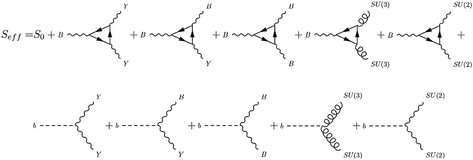
Figure 1. The 1PI effective action for a typical low scale model obtained by adding one extra anomalous U(1)_B to the Standard Model action. Shown are the one-loop trilinear anomalous interactions and the corresponding counterterms, involving the b field.

TABLE 1

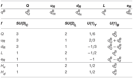
Table 1. Charges of the fermion and of the scalar fields.

4.2. Fermion/Gauge Field Couplings

The models that we discuss are characterized by one extra neutral current, mediated by a Z′ gauge boson. The interaction of the fermions with the gauge fields is defined by the Lagrangian

$\begin{array}{l}{{L}}_{int}^{quarks}=({\bar{u}}_{Li}{\bar{d}}_{Li}){\gamma }^{\mu }\left[-g_s{T}^a{G}_{\mu }^a-g_2{\tau }^a{W}_{\mu }^a-\frac{1}{12}{g}_Y{Y}_{\mu }-\frac{1}{2}{g}_B{q}_Q^B{B}_{\mu }\right]\left(\begin{array}{l}{u}_{Li}\\ d_{Li}\end{array}\right)+\\ +{\bar{u}}_{Ri}{\gamma }^{\mu }\left[-g_s{T}^a{G}_{\mu }^a-g_2{\tau }^a{W}_{\mu }^a-\frac{1}{3}{g}_Y{Y}_{\mu }-\frac{1}{2}{g}_B{q}_{u_R}^B{B}_{\mu }\right]u_{Ri}\\ +{\bar{d}}_{Ri}{\gamma }^{\mu }\left[-g_s{T}^a{G}_{\mu }^a-g_2{\tau }^a{W}_{\mu }^a+\frac{1}{6}{g}_Y{Y}_{\mu }-\frac{1}{2}{g}_B{q}_{d_R}^B{B}_{\mu }\right]d_{Ri}.& (24)\end{array}$

while the Higgs sector is characterized by the two Higgs doublets

$\begin{array}{ll}{H}_u=\left(\begin{array}{l}{H}_u^{+}\\ H_u^0\end{array}\right)H_d=\left(\begin{array}{l}{H}_d^{+}\\ H_d^0\end{array}\right)& (25)\end{array}$

where $H_u^{+}$, $H_d^{+}$ and $H_u^0$, $H_d^0$ are complex fields with (with some abuse of notation we rescale the fields by a factor of $1/\sqrt{2}$)

$\begin{array}{l}{H}_u^{+}=\frac{\mathrm{\text{Re}}{H}_u^{+}+i\mathrm{\text{Im}}{H}_u^{+}}{\sqrt{2}},H_d^{-}=\frac{\mathrm{\text{Re}}{H}_d^{-}+i\mathrm{\text{Im}}{H}_d^{-}}{\sqrt{2}},\\ H_u^{-}=H_u^{+*},H_d^{+}=H_d^{-*}.& (26)\end{array}$

Expanding around the vacuum we get for the neutral components

$\begin{array}{ll}{H}_u^0=v_u+\frac{\mathrm{\text{Re}}{H}_u^0+i\mathrm{\text{Im}}{H}_u^0}{\sqrt{2}},H_d^0=v_d+\frac{\mathrm{\text{Re}}{H}_d^0+i\mathrm{\text{Im}}{H}_d^0}{\sqrt{2}}.& (27)\end{array}$

which will play a key role in determining the mixing of the Stückelberg field in the periodic potential. The electroweak mixing angle is defined by cos θ_W = g₂/g, sin θ_W = g_Y/g, with $g^2=g_Y^2+g_2^2$. We also define cos β = v_d/v, sin β = v_u/v with $v^2=v_d^2+v_u^2$. The matrix rotates the neutral gauge bosons from the interaction to the mass eigenstates after electroweak symmetry breaking and has elements which are O(1), being expressed in terms of ratios of coupling constants, which correspond to mixing angles. It is given by

$\begin{array}{ll}\left(\begin{array}{c}{A}_{\gamma }\\ Z\\ Z^{\prime }\end{array}\right)=O^A\left(\begin{array}{c}{W}_3\\ A^Y\\ B\end{array}\right)& (28)\end{array}$

which can be approximated to leading order as

$\begin{array}{ll}{O}^A\simeq \left(\begin{array}{ccc}\frac{g_Y}{g}& \frac{g_2}{g}& 0\\ \frac{g_2}{g}+O({ϵ}_1^2)& -\frac{g_Y}{g}+O({ϵ}_1^2)& \frac{g}{2}{ϵ}_1\\ -\frac{g_2}{2}{ϵ}_1& \frac{g_Y}{2}{ϵ}_1& 1+O({ϵ}_1^2)\end{array}\right)& (29)\end{array}$

where

$\begin{array}{l}{ϵ}_1=\frac{x_B}{M^2},\\ x_B=(q_u^B{v}_u^2+q_d^B{v}_d^2).& (30)\end{array}$

Once the WZ counterterms rotates into the gauge eigenstates and the b field into the physical χ field, there will be a direct coupling of the anomaly to the physical gauge bosons. This will involve both the neutral and the charged sectors. More details can be found in Corianò et al. [17].

4.3. Counterterms

Fixing the values of the counterterms in simple single U(1) models like the one we are reviewing, allows to gain some insight into the possible solutions of the gauge invariance conditions on the Lagrangian. The numerical values of the counterterms appearing in the second line of Figure 1 are fixed by such conditions, giving

$\begin{array}{l}{C}_{BYY}=-\frac{1}{6}{q}_Q^B+\frac{4}{3}{q}_{u_R}^B+\frac{1}{3}{q}_{d_R}^B-\frac{1}{2}{q}_L^B+q_{e_R}^B,\\ C_{YBB}=-{(q_Q^B)}^2+2{(q_{u_r}^B)}^2-{(q_{d_R}^B)}^2+{(q_L^B)}^2-{(q_{e_R}^B)}^2,\\ C_{BBB}=-6{(q_Q^B)}^3+3{(q_{u_R}^B)}^3+3{(q_{d_R}^B)}^3-2{(q_L^B)}^3+{(q_{e_R}^B)}^3,\end{array}$

$\begin{array}{l}{C}_{Bgg}=\frac{1}{2}(-2q_Q^B+q_{d_R}^B+q_{u_R}^B),\\ C_{BWW}=\frac{1}{2}(-q_L^B-3q_Q^B).& (31)\end{array}$

They are, respectively, the counterterms for the cancellation of the mixed anomaly $U{(1)}_{B}U{(1)}_Y^2$ and $U{(1)}_{Y}U{(1)}_B^2$; the counterterm for the BBB anomaly vertex or $U{(1)}_B^3$ anomaly, and those of the $U{(1)}_{B}SU{(3)}^2$ and $U{(1)}_{B}SU{(2)}^2$ anomalies. From the Yukawa couplings we get the following constraints on the U(1)_B charges

$\begin{array}{ll}{q}_Q^B-q_d^B-q_{d_R}^B=0q_Q^B+q_u^B-q_{u_R}^B=0q_L^B-q_d^B-q_{e_R}^B=0.& (32)\end{array}$

Using the equations above, we can eliminate some of the charges in the expression of the counterterms, obtaining

$\begin{array}{l}{C}_{BYY}=\frac{1}{6}(3q_L^B+9q_Q^B+8\text{Δ}{q}^B),\\ C_{YBB}=2\left[q_d^B(q_L^B+3q_Q^B)+2\text{Δ}{q}^B(q_d^B+q_Q^B)+{(\text{Δ}{q}^B)}^2\right],\\ C_{BBB}={(q_L^B-q_d^B)}^3+3{(q_d^B+q_Q^B+\text{Δ}{q}^B)}^3+3{(q_Q^B-q_d^B)}^3\\ -2{(q_L^B)}^3-6{(q_Q^B)}^3,\\ C_{Bgg}=\frac{\text{Δ}{q}^B}{2},\\ C_{BWW}=\frac{1}{2}(-q_L^B-3q_Q^B).& (33)\end{array}$

The equations above parametrize, in principle, an infinite class of models whose charge assignments under U(1)_B are arbitrary, with the charges in the last column of Table 1 taken as their free parameters. The coupling of the axion to the corresponding gauge bosons can be fixed by a complete solution to the anomaly constraints, which may provide us with an insight into the possible mechanisms of misalignment that could take place at both the electroweak and at the QCD phase transitions.

4.4. Choice of the Charges

Due to the presence, in general, of a nonvanishing mixed anomaly of the U(1)_B gauge factor with both SU(2) and SU(3), the Stückelberg axion of the model has interactions with both the strong and the weak sectors, which both support instanton solutions, and therefore could acquire a mass non-perturbatively both at the electroweak and at the QCD phase transitions. In this case we consider the possibility of having sequential misalignments, with the largest contribution to the mass coming from the latter. Obviously, for a choice of charges characterized by Δq = 0, in which both doublets of the Higgs sector H_u and H_d carry the same charge under U(1)_B, the axion mass will not acquire any instanton correction at the QCD phase transition. In this case the potential responsible for Higgs-axion mixing would vanish. In this scenario a solution to the anomaly equations with a vanishing electroweak interaction of the Stückelberg can be obtained by choosing $q_L^B=-3q_Q^B$.

If instead the charges are chosen in a way to have both non-vanishing weak (C_BWW) and strong (C_Bgg) counterterms, it is reasonable to expect that the misalignment of the axion potential will be sequential, with a tiny mass generated at the electroweak phase transition, followed by a second misalignment induced at the strong phase transition. The instanton configurations of the weak and strong sectors will be contributing differently to the mass of the physical axion. However, due to the presence of a coupling of this field with the strong sector, its mass will be significantly dominated by the QCD phase transition, as in the Peccei-Quinn case.

4.5. The Scalar Sector

The scalar sector of the anomalous abelian models is characterized, as already mentioned, by the ordinary electroweak potential of the SM involving, in the simplest formulation, two Higgs doublets V_PQ(H_u, H_d) plus one extra contribution, denoted as V_PQ(H_u, H_d, b) - or V′ (PQ breaking) in Corianò et al. [14] - which mixes the Higgs sector with the Stückelberg axion b, needed for the restoration of the gauge invariance of the effective Lagrangian

$\begin{array}{ll}V=V_{PQ}(H_u,H_d)+V_{PQ}(H_u,H_d,b).& (34)\end{array}$

The appearance of the physical axion in the spectrum of the model takes place after the phase-dependent terms—here assumed to be of non-perturbative origin and generated at a phase transition—find their way in the dynamics of the model and induce a curvature on the scalar potential. The mixing induced in the CP-odd sector determines the presence of a linear combination of the Stückelberg field b and of the Goldstones of the CP-odd sector which acquires a tiny mass. From (34) we have a first term.

$\begin{array}{l}{V}_{PQ}={\mu }_u^2{H}_u^{†}{H}_u+{\mu }_d^2{H}_d^{†}{H}_d+{\text{λ}}_{uu}{(H_u^{†}{H}_u)}^2+{\text{λ}}_{dd}{(H_d^{†}{H}_d)}^2\\ -2{\text{λ}}_{ud}(H_u^{†}{H}_u)(H_d^{†}{H}_d)+2{\text{λ}}_{ud}^{\prime }|H_u^T{\tau }_2{H}_d{|}^2& (35)\end{array}$

typical of a two-Higgs doublet model, to which we add a second PQ breaking term

$\begin{array}{l}{V}_{PQ}={\text{λ}}_0(H_u^{†}{H}_d{e}^{-i{g}_B(q_u-q_d)\frac{b}{2M}})+{\text{λ}}_1{(H_u^{†}{H}_d{e}^{-i{g}_B(q_u-q_d)\frac{b}{2M}})}^2\\ +{\text{λ}}_2(H_u^{†}{H}_u)(H_u^{†}{H}_d{e}^{-i{g}_B(q_u-q_d)\frac{b}{2M}})+\\ {\text{λ}}_3(H_d^{†}{H}_d)(H_u^{†}{H}_d{e}^{-i{g}_B(q_u-q_d)\frac{b}{2M}})+\mathrm{\text{h.c.}}& (36)\end{array}$

These terms are allowed by the symmetry of the model and are parameterized by one dimensionful (λ₀) and three dimensionless couplings (λ₁, λ₂, λ₃). Their values are weighted by an exponential factor containing as a suppression the instanton action. In the equations below we will rescale λ₀ by the electroweak scale $v=\sqrt{v_u^2+v_d^2}$ (${\text{λ}}_0\equiv {\overline{\text{λ}}}_{0}v$) so as to obtain a homogeneous expression for the mass of χ as a function of the relevant scales of the model which are, besides the electroweak vev v the Stückelberg mass M and the anomalous gauge coupling of the U(1)_B, g_B.

The gauging of an anomalous symmetry has some important effects on the properties of this pseudoscalar, first among all the appearance of independent mass and couplings to the gauge fields. This scenario allows then a wider region of parameter space in which one could look for such particles [15, 17, 20], rendering them “axion-like particles” rather than usual axions. We will still refer to them as axions for simplicity. So far only two complete models have been put forward for a consistent analysis of these types of particles, the first one non-supersymmetric [14] and a second one supersymmetric [22].

4.6. The Potential for a Generic Stückelberg Mass

The physical axion χ emerges as a linear combination of the phases of the various complex scalars appearing in combination with the b field. To illustrate the appearance of a physical direction in the phase of the extra potential, we focus our attention on just the CP-odd sector of the total potential, which is the only one that is relevant for our discussion. The expansion of this potential around the electroweak vacuum is given by the parameterization

$\begin{array}{ll}{H}_u=\left(\begin{array}{c}{H}_u^{+}\\ v_u+H_u^0\end{array}\right)H_d=\left(\begin{array}{c}{H}_d^{+}\\ v_d+H_d^0\end{array}\right).& (37)\end{array}$

where v_u and v_d are the two vevs of the Higgs fields. This potential is characterized by two null eigenvalues corresponding to two neutral Nambu-Goldstone modes $(G_0^1,G_0^2)$ and an eigenvalue corresponding to a massive state with an axion component (χ). In the $(\mathrm{\text{Im}}{H}_d^0,\mathrm{\text{Im}}{H}_u^0,b)$ CP-odd basis we obtain the following normalized eigenstates

$\begin{array}{l}{G}_0^1=\frac{1}{\sqrt{v_u^2+v_d^2}}\left(v_d,v_u,0\right)\\ G_0^2=\frac{1}{\sqrt{g_B^2{\left(q_d-q_u\right)}^2{v}_d^2{v}_u^2+2M^2\left(v_d^2+v_u^2\right)}}\\ \left(-\frac{g_B\left(q_d-q_u\right)v_d{v}_u^2}{\sqrt{v_u^2+v_d^2}},\frac{g_B\left(q_d-q_u\right)v_d^2{v}_u}{\sqrt{v_d^2+v_u^2}},\sqrt{2}M\sqrt{v_u^2+v_d^2}\right)\\ \chi =\frac{1}{\sqrt{g_B^2{\left(q_d-q_u\right)}^2{v}_u^2{v}_d^2+2M^2\left(v_d^2+v_u^2\right)}}\\ \left(\sqrt{2}M{v}_u,-\sqrt{2}M{v}_d,g_B(q_d-q_u)v_d{v}_u\right)& (38)\end{array}$

and we indicate with O^χ the orthogonal matrix which allows to rotate them to the physical basis

$\begin{array}{ll}\left(\begin{array}{c}{G}_0^1\\ G_0^2\\ \chi \end{array}\right)=O^{\chi }\left(\begin{array}{c}\mathrm{\text{Im}}{H}_d^0\\ \mathrm{\text{Im}}{H}_u^0\\ b\end{array}\right),& (39)\end{array}$

which is given by

$\begin{array}{ll}{O}^{\chi }=\left(\begin{array}{ccc}\frac{v_d}{v}& \frac{v_u}{v}& 0\\ -\frac{g_B(q_d-q_u)v_d{v}_u^2}{v\sqrt{g_B^2{(q_d-q_u)}^2{v}_d^2{v}_u^2+2M^2{v}^2}}& \frac{g_B(q_d-q_u)v_d^2{v}_u}{v\sqrt{g_B^2{(q_d-q_u)}^2{v}_d^2{v}_u^2+2M^2{v}^2}}& \frac{\sqrt{2}Mv}{\sqrt{g_B^2{(q_d-q_u)}^2{v}_d^2{v}_u^2+2M^2{v}^2}}\\ \frac{\sqrt{2}M{v}_u}{\sqrt{g_B^2{(q_d-q_u)}^2{v}_u^2{v}_d^2+2M^2{v}^2}}& -\frac{\sqrt{2}M{v}_d}{\sqrt{g_B^2{(q_d-q_u)}^2{v}_u^2{v}_d^2+2M^2{v}^2}}& \frac{g_B(q_d-q_u)v_d{v}_u}{\sqrt{g_B^2{(q_d-q_u)}^2{v}_u^2{v}_d^2+2M^2{v}^2}}\end{array}\right)& (40)\end{array}$

where $v=\sqrt{v_u^2+v_d^2}$.

χ inherits WZ interaction since b can be related to the physical axion χ and to the Nambu-Goldstone modes via this matrix as

$\begin{array}{ll}b=O_{13}^{\chi }{G}_0^1+O_{23}^{\chi }{G}_0^2+O_{33}^{\chi }\chi ,& (41)\end{array}$

or, conversely,

$\begin{array}{ll}\chi =O_{31}^{\chi }\mathrm{\text{Im}}{H}_d+O_{32}^{\chi }\mathrm{\text{Im}}{H}_u+O_{33}^{\chi }b.& (42)\end{array}$

Notice that the rotation of b into the physical axion χ involves a factor $O_{33}^{\chi }$ which is of order v/M. This implies that χ inherits from b an interaction with the gauge fields which is suppressed by a scale M²/v. This scale is the product of two contributions: a 1/M suppression coming from the original Wess-Zumino counterterm of the Lagrangian ($b/MF\tilde{F}$) and a factor v/M obtained by the projection of b into χ due to O_χ.

The direct coupling of the axion to the physical gauge bosons via the Wess-Zumino counterterms is obtained by the usual rotation to the mass eigenstates which can be obtained from the rotation matrix O^A defined in (29). The final expression of the coupling of the axi-Higgs to the photon $g_{\chi \gamma \gamma }\chi F_{\gamma }\widetilde{F_{\gamma }}$, is defined by a combination of matrix elements of the rotation matrices O^A and O^χ. Defining $g^2=g_2^2+g_Y^2$, the expression of this coefficient can be derived in the form

$\begin{array}{ll}{g}_{\gamma \gamma }^{\chi }=\frac{g_B{g}_Y^2{g}_2^2}{32{\pi }^{2}M{g}^2}{O}_{33}^{\chi }{\displaystyle \sum _f}\left(-q_{fL}^B+q_{fR}^B{\left(q_{fR}^Y\right)}^2-q_{fL}^B{\left(q_{fL}^Y\right)}^2\right).& (43)\end{array}$

Notice that this expression is cubic in the gauge coupling constants, since factors such as g₂/g and g_Y/g are mixing angles while the factor 1/π² originates from the anomaly. Therefore, one obtains a general behavior for $g_{\gamma \gamma }^{\chi }$ of O(g³v/M²), with charges which are, in general, of order unity.

4.7. Periodicity of the Extra Potential

Equivalently, it is possible to reobtain the results above by an analysis of the phases of the extra potential, which shows how this becomes periodic in χ, the axi-Higgs. This approach shows also quite directly the gauge invariance of χ as a physical pseudoscalar. In fact, if we opt for a polar parametrization of the neutral components in the broken phase

$\begin{array}{l}{H}_u^0=\frac{1}{\sqrt{2}}\left(\sqrt{2}{v}_u+{\rho }_u^0(x)\right)e^{i\frac{F_u^0(x)}{\sqrt{2}{v}_u}}\\ H_d^0=\frac{1}{\sqrt{2}}\left(\sqrt{2}{v}_d+{\rho }_d^0(x)\right)e^{i\frac{F_d^0(x)}{\sqrt{2}{v}_d}},& (44)\end{array}$

where we have introduced the two phases F_u and F_d of the two neutral Higgs fields, information on the periodicity is obtained by combining all the phases of V′

$\begin{array}{ll}\theta (x)\equiv \frac{g_B(q_d-q_u)}{2M}b(x)-\frac{1}{\sqrt{2}{v}_u}{F}_u^0(x)+\frac{1}{\sqrt{2}{v}_d}{F}_d^0(x).& (45)\end{array}$

Using the matrix O^χ to rotate on the physical basis of the CP-odd scalar sector, the phase describing the periodicity of the potential turns out to be proportional to the physical axion χ, modulo a dimensionful constant (σ_χ)

$\begin{array}{ll}\theta (x)\equiv \frac{\chi (x)}{{\sigma }_{\chi }},& (46)\end{array}$

where we have defined

$\begin{array}{ll}{\sigma }_{\chi }\equiv \frac{2v_u{v}_{d}M}{\sqrt{g_B^2{(q_d-q_u)}^2{v}_d^2{v}_u^2+2M^2(v_d^2+v_u^2)}}.& (47)\end{array}$

Notice that σ_χ, in our case, takes the role of f_a of the PQ case, where the angle of misalignment is identified by the ratio a/f_a, with a the PQ axion.

As already mentioned, the re-analysis of the V′ potential is particularly useful for proving the gauge invariance of χ under a U(1)_B infinitesimal gauge transformation with gauge parameter α_B(x). In this case one gets

$\begin{array}{l}\delta H_u=-\frac{i}{2}{q}_u{g}_B{\alpha }_B{H}_u\\ \delta H_d=-\frac{i}{2}{q}_d{g}_B{\alpha }_B{H}_d\\ \delta F_0^u=-\frac{v_u}{\sqrt{2}}{q}_u{g}_B{\alpha }_B\\ \delta F_0^d=-\frac{v_d}{\sqrt{2}}{q}_d{g}_B{\alpha }_B\\ \delta b=-M-S{\alpha }_B& (48)\end{array}$

giving for (46) δθ = 0. The gauge invariance under U(1)_Y can also be easily proven using the invariance of the Stückelberg field b under the same gauge group, sand the fact that the hypercharges of the two Higgses are equal. Finally, the invariance under SU(2) is obvious since the linear combination of the phases that define θ(x) are not touched by the transformation.

From the Peccei-Quinn breaking potential we can extract the following periodic potential

$\begin{array}{ll}{V}^{\prime }=4v_u{v}_d\left({\text{λ}}_2{v}_d^2+{\text{λ}}_3{v}_u^2+{\text{λ}}_0\right)cos\left(\frac{\chi }{{\sigma }_{\chi }}\right)+2{\text{λ}}_1{v}_u^2{v}_d^{2}cos\left(2\frac{\chi }{{\sigma }_{\chi }}\right),& (49)\end{array}$

with a mass for the physical axion χ given by

$\begin{array}{ll}{m}_{\chi }^2=\frac{2v_u{v}_d}{{\sigma }_{\chi }^2}\left({\overline{\text{λ}}}_0{v}^2+{\text{λ}}_2{v}_d^2+{\text{λ}}_3{v}_u^2+4{\text{λ}}_1{v}_u{v}_d\right)\approx \text{λ}{v}^2.& (50)\end{array}$

The size of the potential is driven by the combined product of non-perturbative effects, due to the exponentially small parameters $(\overline{{\text{λ}}_0},{\text{λ}}_1,{\text{λ}}_2,{\text{λ}}_3)$, with the electroweak vevs of the two Higgses. Notice also the irrelevance of the Stückelberg scale M in determining the value of σ_χ ~ O(v) and of m_χ near the transition region, due to the large suppression factor λ in Equation (97). One point that needs to be stressed is the fact that at the electroweak epoch the angle of misalignment generated by the extra potential is parameterized by χ/σ_χ, while the interaction of the physical axion with the gauge fields is suppressed by M²/v. This feature is obviously unusual, since in the PQ case both scales reduce to a single scale, the axion decay constant f_a.

4.8. The Yukawa Couplings and the Axi-Higgs

The Yukawa couplings determine an interaction of the axi-Higgs to the fermions. This interaction is generated by the rotation in the CP-odd sector of the scalars potential, which mixes the CP-odd components, with the inclusion of the Stückelberg b, via the matrix O_χ. The Yukawa couplings of the model are given by

$\begin{array}{l}{{L}}_{\text{Yuk}}^{unit.}=-{\text{Γ}}^d\bar{Q}{H}_d{d}_R-{\text{Γ}}^d{\bar{d}}_R{H}_d^{†}Q-{\text{Γ}}^u{\bar{Q}}_L(i{\sigma }_2{H}_u^{*})u_R-{\text{Γ}}^u{\bar{u}}_R{(i{\sigma }_2{H}_u^{*})}^{†}{Q}_L\\ -{\text{Γ}}^e\bar{L}{H}_d{e}_R-{\text{Γ}}^e{ē}_R{H}_d^{†}L\\ =-{\text{Γ}}^d\bar{d}{H}_d^0{P}_{R}d-{\text{Γ}}^d\bar{d}{H}_d^{0*}{P}_{L}d-{\text{Γ}}^u\bar{u}{H}_u^{0*}{P}_{R}u-{\text{Γ}}^u\bar{u}{H}_u^0{P}_{L}u\\ -{\text{Γ}}^eēH_d^0{P}_{R}e-{\text{Γ}}^eēH_d^{0*}{P}_{L}e,& (51)\end{array}$

where the Yukawa coupling constants Γ^d, Γ^u and Γ^e run over the three generations, i.e., u = {u, c, t}, d = {d, s, b} and e = {e, μ, τ}. Rotating the CP-odd and CP-even neutral sectors into the mass eigenstates and expanding around the vacuum one obtains

$\begin{array}{l}{H}_u^0=v_u+\frac{Re{H}_u^0+iIm{H}_u^0}{\sqrt{2}}\\ =v_u+\frac{(h^{0}sin\alpha -H^{0}cos\alpha )+i\left(O_{11}^{\chi }{G}_0^1+O_{21}^{\chi }{G}_0^2+O_{31}^{\chi }\chi \right)}{\sqrt{2}}& (52)\end{array}$

$\begin{array}{l}{H}_d^0=v_d+\frac{Re{H}_d^0+iIm{H}_d^0}{\sqrt{2}}\\ =v_d+\frac{(h^{0}cos\alpha +H^{0}sin\alpha )+i\left(O_{12}^{\chi }{G}_0^1+O_{22}^{\chi }{G}_0^1+O_{32}^{\chi }\chi \right)}{\sqrt{2}}& (53)\end{array}$

where the vevs of the two neutral Higgs bosons v_u = vsin β and v_d = vcos β satisfy

$\begin{array}{ll}tan\beta =\frac{v_u}{v_d},v=\sqrt{v_u^2+v_d^2}.& (54)\end{array}$

The fermion masses are given by

$\begin{array}{l}{m}_u=v_u{\text{Γ}}^u,m_{\nu }=v_u{\text{Γ}}^{\nu },\\ m_d=v_d{\text{Γ}}^d,m_e=v_d{\text{Γ}}^e,& (55)\end{array}$

where the generation index has been suppressed. The fermion masses, defined in terms of the two expectation values v_u, v_d of the model, show an enhancement of the down-type Yukawa couplings for large values of tan β while at the same time the up-type Yukawa couplings get a suppression. The couplings of the h⁰ boson to fermions are given by

$\begin{array}{l}{{L}}_{\text{Yuk}}(h^0)=-{\text{Γ}}^d{\bar{d}}_L{d}_R\left(\frac{cos\alpha }{\sqrt{2}}{h}^0\right)-{\text{Γ}}^u{\bar{u}}_L{u}_R\left(\frac{sin\alpha }{\sqrt{2}}{h}^0\right)\\ -{\text{Γ}}^e{\bar{e}}_L{e}_R\left(\frac{cos\alpha }{\sqrt{2}}{h}^0\right)+c.c.& (56)\end{array}$

The couplings of the H⁰ boson to the fermions are

$\begin{array}{l}{{L}}_{\text{Yuk}}(H^0)=-{\text{Γ}}^d{\bar{d}}_L{d}_R\left(\frac{sin\alpha }{\sqrt{2}}{H}^0\right)-{\text{Γ}}^u{\bar{u}}_L{u}_R\left(-\frac{cos\alpha }{\sqrt{2}}{H}^0\right)\\ -{\text{Γ}}^e{\bar{e}}_L{e}_R\left(\frac{sin\alpha }{\sqrt{2}}{H}^0\right)+c.c.& (57)\end{array}$

The interaction of χ with the fermions is proportional to the rotation matrix O^χ and to the mass of the fermion. The decay of the axi-Higgs is driven by two contributions, the direct point-like WZ interaction $(\chi /MF\tilde{F})$ and the fermion loop. The amplitude can be separated in the form corresponding to the two contributions from diagrams of Figures 2A,B

$\begin{array}{ll}{{M}}^{\mu \nu }(\chi \to \gamma \gamma )={{M}}_{WZ}^{\mu \nu }+{{M}}_f^{\mu \nu }.& (58)\end{array}$

FIGURE 2

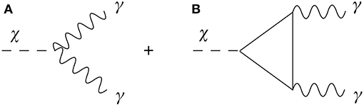
Figure 2. Contributions to the χ → γγ decay. describing the anomaly contribution (A) and the interaction mediated by the Yukava coupling in the fermion loop (B).

The direct coupling related to the anomaly is given by the vertex shown in Figure 2A

$\begin{array}{ll}{{M}}_{WZ}^{\mu \nu }(\chi \to \gamma \gamma )=4g_{\gamma \gamma }^{\chi }\epsilon \left[\mu ,\nu ,k_1,k_2\right]& (59)\end{array}$

coming from the WZ counterterm $\chi F_{\gamma }{\tilde{F}}_{\gamma }$ which gives a decay rate of the form

$\begin{array}{ll}{\text{Γ}}_{WZ}(\chi \to \gamma \gamma )=\frac{m_{\chi }^3}{4\pi }{(g_{\gamma \gamma }^{\chi })}^2.& (60)\end{array}$

We remark that $g_{\gamma \gamma }^{\chi }$ is of O(g³v/M²), as derived from Equation (43), with charges that have been chosen of O(1). It is

Comparative studies of the decay rate into photons for the axi-Higgs with the ordinary PQ axion have been performed for a Stückelberg scale confined in the TeV range and a mass of χ in the same range expected for the PQ axion. The analysis shows that the total decay rate of χ into photons is of the order ${\text{Γ}}_{\chi }~10^{-50}$ GeV, which is larger than the decay rate of the PQ axion in the same channel (10⁻⁶⁰), but small enough to be long- lived, with a lifetime larger than the age of the universe. We show in Figure 3 the result of this study, where we compare predictions for the decay rate of the axi-Higgs into two photons to that of the ordinary PQ axion.

FIGURE 3

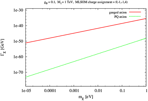
Figure 3. Total decay rate of the axi-Higgs for several mass values. Here, for the PQ axion, we have chosen $f_a=10^{10}$ GeV.

The charge assignment of the anomalous model has been denoted as f(−1, 1, 4), where we have used the convention

$\begin{array}{ll}f(q_{Q_L}^B,q_L^B,\text{Δ}{q}^B)\equiv (q_{Q_L}^B,q_{u_R}^B;q_{d_R}^B,q_L^B,q_{e_R}^B,q_u^B,q_d^B).& (61)\end{array}$

These depend only upon the three free parameters $q_{Q_L}^B$, $q_L^B,\text{Δ}{q}^B$. The parametric solution of the anomaly equations of the model $f(q_{Q_L}^B,q_L^B,\text{Δ}{q}^B)$, for the particular choice $q_{Q_L}^B=-1,q_L^B=-1$, reproduces the entire charge assignment of a special class of intersecting brane models (see [29, 32] and the discussion in Corianò and Guzzi [20])

$\begin{array}{ll}f(-1,-1,4)=(-1,0,0,-1,0,+2,-2).& (62)\end{array}$

We refer to Corianò et al. [12] for further details on these studies.

5. Relic Density for a Low (~ 1 TeV) Stückelberg Scale

The computation of the relic density for the Stückelberg axi-Higgs can be performed as in Corianò et al. [13], adopting a low scale scenario, where the extra V′ (49) potential which causes the vacuum misalignment is generated around the electroweak scale.

One starts from the Lagrangian

$\begin{array}{ll}{S}={\displaystyle \int d^{4}x\sqrt{g}\left(\frac{1}{2}{\dot{\chi }}^2-\frac{1}{2}{m}_{\chi }^2{\text{Γ}}_{\chi }\dot{\chi }\right),}& (63)\end{array}$

where Γ_χ is the decay rate of the axion, where the potential has been expanded around its minimum up to quadratic terms. The same action can be derived from the quadratic approximation to the general expression

$\begin{array}{ll}{S}={\displaystyle \int d^{4}x{R}^3(t)\left(\frac{1}{2}{\sigma }_{\chi }^2{({\partial }_{\alpha }\theta )}^2-{\mu }^4(1-cos\theta )-V_0\right)}& (64)\end{array}$

which, as just mentioned, is constructed from the expression of V′ given in Equation (49). Here μ ~ v, is the electroweak scale. We also set other contributions to the vacuum potential to zero (V₀ = 0). In a Friedmann-Robertson-Walker spacetime metric, with a scaling factor R(t), this action gives the equation of motion

$\begin{array}{ll}\frac{d}{dt}[\left(R^3\left(t\right)\left(\dot{\chi }+{\text{Γ}}_{\chi }\right)\right]+R^3{m}_{\chi }^2\left(T\right)=0.& (65)\end{array}$

We will neglect the decay rate of the axion in this case and set Γ_χ ≈ 0. At this point, we are free to set the scale at which the V′ potential, which is of non-perturbative origin, is generated. Therefore, it will be zero above the electroweak scale (or temperature T_ew), which will give m_χ = 0 for T ≫ T_ew. The general equation of motion derived from Equation (65), introducing a temperature dependent mass, can be written as

$\begin{array}{ll}\ddot{\chi }+3H\dot{\chi }+m_{\chi }^2(T)\chi =0,& (66)\end{array}$

which allows as a solution a constant value of the misalignment angle θ = θ_i. The axion energy density is given by

$\begin{array}{ll}\rho =\frac{1}{2}{\dot{\chi }}^2+\frac{1}{2}{m}_{\chi }^2{\chi }^2,& (67)\end{array}$

which after a harmonic averaging, due to the periodic motion, gives

$\begin{array}{ll}\text{〈}\rho \text{〉}=m_{\chi }^2\text{〈}{\chi }^2\text{〉}.& (68)\end{array}$

By differentiating Equation (67) and using the equation of motion in (66), followed by the averaging Equation (68) one obtains the relation

$\begin{array}{ll}\text{〈}\dot{\rho }\text{〉}=\text{〈}\rho \text{〉}\left(-3H+\frac{\dot{m}}{m}\right),& (69)\end{array}$

with a mass which is time-dependent through its temperature T(t), while H(t) = $\dot{R}$(t)/R(t) is the Hubble parameter. One easily finds that the solution of this equation is of the form

$\begin{array}{ll}\text{〈}\rho \text{〉}=\frac{m_{\chi }(T)}{R^3(t)}& (70)\end{array}$

which shows the decay of the energy density with an increasing space volume, valid even for a T-dependent mass. The condition for the oscillations of χ to take place is that the universe has to at least be as old as the period of oscillation. Then the axion field starts oscillating and appears as dark matter, otherwise θ is misaligned but frozen. This is the physical content of the condition

$\begin{array}{ll}{m}_{\chi }(T_i)=3H(T_i),& (71)\end{array}$

which allows to identify the initial temperature of the coherent oscillation of the axion field χ, T_i, by equating m_χ(T) to the Hubble rate, taken as a function of temperature.

In the radiation era, the thermodynamics of all the components of the primordial state is entirely determined by the temperature T, being the system at equilibrium. This is because the contents of the early universe were in approximate thermal equilibrium, being the interaction rates of the constituents were large compared to the interaction rates H.

Pressure and entropy are then just given as a function of the temperature

$\begin{array}{l}\rho =3p=\frac{{\pi }^2}{30}{g}_{*,T}{T}^4\\ s=\frac{2{\pi }^2}{45}{g}_{*,S,T}{T}^3.& (72)\end{array}$

Combined with the Friedmann equation they allow to relate the Hubble parameter and the energy density

$\begin{array}{ll}H=\sqrt{\frac{8}{3}\pi G_N\rho },& (73)\end{array}$

with $G_N=1/M_P^2$ being the Newton constant and M_P the Planck mass. The number density of axions n_χ decreases as 1/R³ with the expansion, as does the entropy density s ≡ S/R³, where S indicates the comoving entropy density, which remains constant in time, leaving the ratio Y_a ≡ n_χ/s conserved. An important variable is the abundance of χ at the temperature of oscillations T_i, which is defined as

$\begin{array}{ll}{Y}_{\chi }(T_i)={\displaystyle \frac{n_{\chi }}{s}{|}_{T_i}.}& (74)\end{array}$

At the beginning of the oscillations the total energy density is just the potential one

$\begin{array}{ll}{\rho }_{\chi }=n_{\chi }(T_i)m_{\chi }(T_i)=1/2m_{\chi }^2(T_i){\chi }_i^2,& (75)\end{array}$

giving for the initial abundance at T = T_i

$\begin{array}{ll}{Y}_{\chi }(T_i)=\frac{1}{2}\frac{m_{\chi }(T_i){\chi }_i^2}{s}=\frac{45m_{\chi }(T_i){\chi }_i^2}{4{\pi }^2{g}_{*,S,T}{T}_i^3}& (76)\end{array}$

where we have used the expression of the entropy given by Equation (72). At this point, by inserting the expression of ρ given in Equation (72) into the expression of the Hubble rate as a function of density given by Equation (73), the condition for oscillation Equation (71) allows to express the axion mass at T = T_i in terms of the effective massless degrees of freedom evaluated at the same temperature

$\begin{array}{ll}{m}_{\chi }(T_i)=\sqrt{\frac{4}{5}{\pi }^3{g}_{*,T_i}}\frac{T_i^2}{M_P}.& (77)\end{array}$

This gives for Equation (76) the expression

$\begin{array}{ll}{Y}_{\chi }(T_i)=\frac{45{\sigma }_{\chi }^2{\theta }_i^2}{2\sqrt{5\pi g_{*,T_i}}{T}_i{M}_P},& (78)\end{array}$

where we have expressed χ in terms of the angle of misalignment θ_i at the temperature when oscillations start. Notice that we are assuming that θ_i = 〈θ〉 is the zero mode of the initial misalignment angle after an averaging.

g_{*, T} = 110.75 is the number of massless degrees of freedom of the model at the electroweak scale. Using the conservation of the abundance Y_a0 = Y_a(T_i), the expression of the contribution to the relic density is given by

$\begin{array}{ll}{\text{Ω}}_{\chi }^{mis}={\displaystyle \frac{n_{\chi }}{s}{|}_{T_i}{m}_{\chi }\frac{s_0}{{\rho }_c}.}& (79)\end{array}$

To evaluate (79) we need the values of the critical energy density (ρ_c) and the entropy density today, which are estimated as

$\begin{array}{ll}{\rho }_c=5.2·10^{-6}\mathrm{\text{GeV}}/{\mathrm{\text{cm}}}^3{s}_0=2970{\mathrm{\text{ cm}}}^{-3},& (80)\end{array}$

with θ ≃ 1. Given these values, the relic density as a function of tan β = v_u/v_d, the ratio of the two Higgs vevs, is given in Figure 4. In this plot we have varied the oscillation mass and plotted the relic densities as a function of this variable. The variation of v_u has been constrained to give the values of the masses of the electroweak gauge bosons, via an appropriate choice of tan β.

FIGURE 4

Figure 4. Relic density of the axi-Higgs as a function of tan β for several values of the mass of the axi-Higgs.

For instance, if we assume a temperature of oscillation of T_i = 100 GeV, an upper bound for the axi-Higgs mass, which allows the oscillations to take place, is $m_{\chi }(T_i)\approx 10^{-5}\mathrm{\text{eV}}$, with g_{*, T} ≈ 100.

In order to specify σ_χ we have assumed a value of 1 TeV for the Stückelberg mass M_S, with a gauge coupling of the anomalous B_μ, g_B ≈ 1, and we have taken (q_u, q_d) of order unity, obtaining ${\sigma }_{\chi }\simeq 10^2$ GeV. As we lower the oscillation temperature (and hence the mass), the corresponding curves for Ω_χ are down-shifted.

The plot shows that the values of these relic densities at current time are basically vanishing and these small results are to be attributed to the value of σ_χ, which is bound to vary around the electroweak scale. We remind that in the PQ case σ_χ is replaced by the large scale f_a at the QCD phase transition, which determines an enhancement of Ω_χ respect to the current case.

As already mentioned, nonperturbative instanton effects at the electroweak scale are expected to vastly suppress the mass of the axi-Higgs, as derived in (97), in the form

$\begin{array}{ll}{m}_{\chi }^2~{\text{Λ}}_{ew}^4/v^2,\mathrm{\text{with }}{\text{Λ}}_{ew}^4~\mathrm{\text{Exp}}(-2\pi /{\alpha }_w(v))v^4& (81)\end{array}$

α_W(v) being the weak charge at the scale v- which is indeed a rather small value since $\mathrm{\text{Exp}}(-2\pi /{\alpha }_w(v))~e^{-198}$. We will come back to this point in the next section, when discussing the possibility of raising M_S from the TeV range up to the GUT or Planck scales.

For this reason, χ essentially remains a physical but frozen degree of freedom which may undergo a significant (second) misalignment only at the QCD phase transition. The possibility of sequential misalignments has been taken into account both in non-supersymmetric [12] and in supersymmetric models [13]. It is the presence of a coupling of the axion to the gluons, via the color/ U(1)_B mixed anomaly, that χ behaves, in this case, similar to a PQ axion. The misalignment is controlled by the periodic potential generated at the QCD phase transition, being the first misalignment at the electroweak scale irrelevant. In the absence of such mixed anomaly, χ could be classified as a quintessence axion, contributing to the dark energy content of the universe.

We show in Figure 5 results of a numerical study of ${\text{Ω}}_{mis}{h}^2$ as a function of M_S, expressed in units of 10⁹ GeV. We show as a darkened area the bound coming from WMAP data [35], given as the average value plus an error band, while the monotonic curve denotes the values of ${\text{Ω}}_{mis}{h}^2$ as a function of M_S. It is clear that the relic density of χ can contribute significantly to the dark matter content only if the Stückelberg scale is rather large (~ 10⁷ GeV) and negligible otherwise.

FIGURE 5

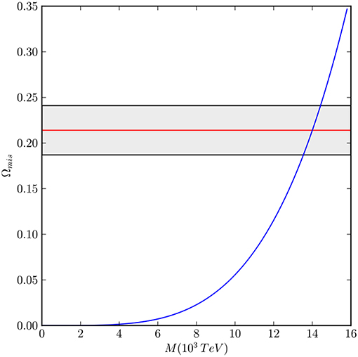
Figure 5. Relic density of the axi-Higgs as a function of M. The gray bar represents the measured value of ${\text{Ω}}_{DM}{h}^2=0.1123\pm 0.0035$.

In the next section we address another scenario, where we will assume that the Stückelberg scale is around the Planck scale and the breaking of the symmetry which allows a periodic potential for the b field to generate, taken at the GUT scale. This particular choice for the location of the two scales, which is well motivated in a string/brane theory context, opens up the possibility of having an ultra-light axion in the spectrum. The De Broglie wavelength of this hypothetical particle would be around 10 kpc, which is what is required to solve the issues in the modeling of the matter distribution at the sub-galactic scale, that we have discussed in the introduction.

6. Stückelberg Models at the Planck/GUT Scale and Fuzzy Dark Matter

By raising the Stückelberg mass near the Planck scale, the Stückelberg construction acquires a fundamental meaning since it can be directly related to the cancellation of a gauge anomaly generated at the same scale [7]. As mentioned above, anomalous U(1) symmetries are quite generally present in theories of intersecting branes. However, the very same structure emerges also in the low energy limit of heterotic string constructions. At the same time, as shown in Corianò et al. [14], even in the presence of multiple anomalous abelian symmetries, only a single axion is necessary to cancel all anomalies, giving a special status to the Stückelberg field. These considerations define a new context in which to harbor such models. In this context, it is natural to try to identify a consistent formulation within an ordinary gauge theory, by assuming that the axion emerges at the Planck scale M_P, but it acquires a mass at a scale below, which in our case is assumed to be the GUT scale. In this section therefore we are going to consider an extension of the setup discussed in previous sections, under the assumption that their dynamics is now controlled by two scales.

We will consider an E₆ based model, derived from E₈, which appeared in the heterotic string construction of Gross et al. [36] with an E(8) × E(8) symmetry. After a compactification of six spatial dimensions on a Calabi-Yau manifold [37] the symmetry is reduced to an E(6) GUT gauge theory. Other string theory compactifications predict different GUT gauge structures, such as SU(5) and SO(10). The E₆, however, allows to realize a scenario where two components of dark matter are present, as we are going to elaborate. Fermions are assigned to the 27 representation of E(6), which is anomaly-free. Notice that in E(6) a PQ symmetry is naturally present, as shown in Frampton and Kephart [11], which allows to have an ordinary PQ axion, while at the same time it is a realistic GUT symmetry which can break to the SM. This is the gauge structure to which one may append an anomalous U(1)_X symmetry.

We consider a gauge symmetry of the form E₆ × U(1)_X, where the gauge boson B^μ is in the Stückelberg phase. B_α is the gauge field of U(1)_X and B_αβ ≡ ∂_αB_β − ∂_βB_α the corresponding field strength, while g_B its gauge coupling. As already mentioned, the U(1)_X carries an anomalous coupling to the fermion spectrum.

The one-particle irreducible (1PI) effective Lagrangian of the theory at 1-loop level takes the form

$\begin{array}{ll}{L}={{L}}_{E_6}+{{L}}_{St}+{{L}}_{anom}+{{L}}_{WZ},& (82)\end{array}$

in terms of the gauge contribution of E₆ (${L}$_E6), the Stückelberg term ${L}$_St, the anomalous 3-point functions ${L}$_anom, generated by the anomalous fermion couplings to the U(1)_X gauge boson, and the Wess-Zumino counterterm (WZ) ${L}$_WZ. The Stückelberg interaction to the E₆ gauge Lagrangian

$\begin{array}{ll}{{L}}_{E_6}=-\frac{1}{4}{F}^{(E_6)\mu \nu }{F}_{\mu \nu }^{(E_6)},& (83)\end{array}$

which enables us to write the Stückelberg part of the Lagrangian as

$\begin{array}{ll}{{L}}_{Stueck}=-\frac{1}{4}{B}_{\alpha \beta }{B}^{\alpha \beta }-\frac{1}{2}{(M{B}_{\alpha }-{\partial }_{\alpha }b(x))}^2.& (84)\end{array}$

In this final form, M is the mass of the Stückelberg gauge boson associated with U(1)_X which we can be taken from the order of the Planck scale, guaranteeing the decoupling of the axion around M_GUT, due to the gravitational suppression of the WZ counterterms. The WZ contribution is the combination of two terms

$\begin{array}{ll}{{L}}_{WZ}=c_1\frac{b}{M}{F}^{(E_6)\mu \nu }{F}^{(E_6)\rho \sigma }{ϵ}_{\mu \nu \rho \sigma }+c_2\frac{b}{M}{B}_{\mu \nu }{B}_{\rho \sigma }{ϵ}^{\mu \nu \rho \sigma }& (85)\end{array}$

needed for the cancellation of the U(1)_XE₆E₆ and $U{(1)}_X^3$ anomalies, for appropriate values of the numerical constants c₁ and c₂, fixed by the charge assignments of the model. The three chiral families will be assigned under E(6) × U(1)_X respectively to

$\begin{array}{ll}{27}_{X_1}{27}_{X_2}{27}_{X_3},& (86)\end{array}$

in which the charges X_i (i = 1, 2, 3) are free at the moment, while the cancellation of the $U{(1)}_X^3$ and $E_6\times U{(1)}_X^2$ anomalies implies that

$\begin{array}{ll}{\displaystyle \sum _{i=1}^3}{X}_i^3=0,{\displaystyle \sum _{i=1}^3}{X}_i=0.& (87)\end{array}$

These need to be violated in order to compensate with a Wess-Zumino term for the restoration of the gauge symmetry of the action.

Concerning the scalar sector, this contains two 351_Xi (i = 1, 2) irreducible representations, where the U(1)_X charges X_i need to be determined. The 351 is the antisymmetric part of the Kronecker product 27 ⊗ 27 where 27 is the defining representation of E(6). The 351_X can be conveniently described by the 2-form A_μν = −A_νμ with μ, ν = 1 to 27. The most general renormalizable potential in ${L}$_E6 is expressed in terms of $A_{\mu \nu }^{(1)}$ and $A_{\mu \nu }^{(2)}$ of U(1)_X of charges x₁ and x₂ respectively. If we denote the 27_Xi of Equation (86) by Ψ_μ with μ = 1 to 27 then the full Lagrangian including the potential V, has an invariance under the global symmetry

$\begin{array}{ll}{A}_{\mu \nu }^{(1)}\to e^{i\theta }{A}_{\mu \nu }^{(1)}{A}_{\mu \nu }^{(2)}\to e^{i\theta }{A}_{\mu \nu }^{(2)}{\text{Ψ}}_{\mu }\to e^{-(\frac{1}{2}i\theta )}{\text{Ψ}}_{\mu }.& (88)\end{array}$

This is identifiable as a Peccei-Quinn symmetry which is broken at the GUT scale when E(6) is broken to SU(5) [11]. This axionic symmetry can be held responsible for solving the strong CP problem. We couple $A_{\mu \nu }^{(1)}$ to the fermion families (27)_Xi i = 1, 2, 3. We choose in Equation (86), e.g., X₁ = X₂ = X₃ = +1, with the X-charge of A⁽¹⁾ fixed to X = −2. The second scalar representation A⁽²⁾ is decoupled from the fermions, with an X−charge for A⁽²⁾ which is arbitrary and taken for simplicity to be X = +2. The potential is expressed in terms of three E₆ × U(1)_X invariant components,

$\begin{array}{ll}V=V_1+V_2+V_p,& (89)\end{array}$

where

$\begin{array}{ll}{V}_1=F(A^{(1)},A^{(1)})V_2=F(A^{(2)},A^{(2)}),& (90)\end{array}$

with V₁ and V₂ denoting the contributions of (351)₋₂ and (351)₊₂, expressed in terms of the function [11]

$\begin{array}{l}F(A^{(i)},A^{(j)})=M_{GUT}^2{A}_{\mu \nu }^{(i)}{\overline{A^{(j)}}}^{\mu \nu }+h_1{(A_{\mu \nu }^{(i)}{\overline{A^{(j)}}}^{\mu \nu })}^2+h_2{A}_{\mu \nu }^{(i)}{\bar{A}}^{\nu \sigma }{A}_{\sigma \tau }^{(i)}{\bar{A}}^{\tau \mu }\\ +h_3{d}^{\mu \nu \text{λ}}{d}_{\xi \eta \text{λ}}{A}_{\mu \sigma }^{(i)}{A}_{\nu \tau }^{(i)}{\overline{A^{(j)}}}^{\xi \sigma }{\overline{A^{(j)}}}^{\eta \tau }\\ +h_4{d}^{\mu \nu \alpha }{d}^{\sigma \tau \beta }{d}_{\xi \eta \alpha }{d}_{\text{λ}\rho \beta }{A}_{\mu \sigma }^{(i)}{A}_{\nu \tau }^{(i)}{\overline{A^{(j)}}}^{\xi \text{λ}}{\overline{A^{(j)}}}^{\eta \rho }\\ +h_5{d}^{\mu \nu \alpha }{d}^{\sigma \beta \gamma }{d}_{\xi \eta \beta }{d}_{\text{λ}\alpha \gamma }{A}_{\mu \sigma }^{(i)}{A}_{\nu \tau }^{(i)}{\overline{A^{(j)}}}^{\xi \text{λ}}{\overline{A^{(j)}}}^{\eta \tau }\\ +h_6{d}^{\mu \nu \alpha }{d}^{\sigma \tau \beta }{d}_{\alpha \beta \gamma }{d}^{\gamma \zeta \xi }{d}_{\xi \eta \zeta }{d}_{\text{λ}\rho \chi }{A}_{\mu \sigma }^{(i)}{\overline{A^{(j)}}}^{\xi \text{λ}}{A}_{\nu \tau }^{(i)}{\overline{A^{(j)}}}^{\eta \rho },& (91)\end{array}$

in which d_αβγ with α, β, γ = 1 to 27 is the E(6) invariant tensor.

As for the two Higgs doublet model discussed in the previous sections, also in this case we are allowed to introduce a periodic potential on the basis of the underlying gauge symmetry, of the form

$\begin{array}{l}{V}_p=M_{GUT}^2{A}_{\mu \nu }^{(1)}{\overline{A^{(2)}}}^{\mu \nu }{e}^{-i4\frac{b}{M_S}}+e^{-i8\frac{b}{M_S}}[(h_1{(A_{\mu \nu }^{(1)}{\overline{A^{(2)}}}^{\mu \nu })}^2+h_2{A}_{\mu \nu }^{(1)}{\overline{A^{(2)}}}^{\nu \sigma }\\ A_{\sigma \tau }^{(1)}{\overline{A^{(2)}}}^{\tau \mu }+h_3{d}^{\mu \nu \text{λ}}{d}_{\xi \eta \text{λ}}{A}_{\mu \sigma }^{(1)}{A}_{\nu \tau }^{(1)}{\overline{A^{(2)}}}^{\xi \sigma }{\overline{A^{(2)}}}^{\eta \tau }\\ +h_4{d}^{\mu \nu \alpha }{d}^{\sigma \tau \beta }{d}_{\xi \eta \alpha }{d}_{\text{λ}\rho \beta }{A}_{\mu \sigma }^{(1)}{A}_{\nu \tau }^{(1)}{\overline{A^{(2)}}}^{\xi \text{λ}}{\overline{A^{(2)}}}^{\eta \rho }\\ +h_5{d}^{\mu \nu \alpha }{d}^{\sigma \beta \gamma }{d}_{\xi \eta \beta }{d}_{\text{λ}\alpha \gamma }{A}_{\mu \sigma }^{(1)}{A}_{\nu \tau }^{(1)}{\overline{A^{(2)}}}^{\xi \text{λ}}{\overline{A^{(2)}}}^{\eta \tau }\\ {\displaystyle +h_6{d}^{\mu \nu \alpha }{d}^{\sigma \tau \beta }{d}_{\alpha \beta \gamma }{d}^{\gamma \zeta \xi }{d}_{\xi \eta \zeta }{d}_{\text{λ}\rho \chi }{A}_{\mu \sigma }^{(1)}{\overline{A^{(2)}}}^{\xi \text{λ}}{A}_{\nu \tau }^{(1)}{\overline{A^{(2)}}}^{\eta \rho }]+h.c.}& (92)\end{array}$

and which become periodic at the GUT scale after symmetry breaking, similar to the case considered in Corianò et al. [12] and Corianò et al. [13]. This potential is expected to be of nonperturbative origin and generated at the scale of the GUT phase transition. Additionally, in this case the size of the contributions in V_p, generated by instanton effects at the GUT scale, are expected to be exponentially suppressed, however, the size of the suppression is related to the value of the gauge coupling at the corresponding scale.

6.1. The Periodic Potential

The breaking of the E₆ × U(1)_X symmetry at M_GUT can follow different routes such as E(6) ⊃ SU(3)_C × SU(3)_L × SU(3)_H where

$\begin{array}{l}(351)=(1,3^{*},3)+(1,3^{*},6^{*})+(1,6,3)+(3,3,1)+(3,6^{*},1)\\ +(3,3,8)+(3^{*},1,3^{*})+(3^{*},1,6)+(3^{*},8,3^{*})+(6^{*},3,1)\\ +(6,1,3^{*})+(8,3^{*},3)& (93)\end{array}$

of which the color singlets are only the 45 states for each of the two (351)_Xi

$\begin{array}{ll}{(1,3^{*},3)}_{X_i}{(1,3^{*},6^{*})}_{X_i}{(1,6,3)}_{X_I}i=1,2.& (94)\end{array}$

One easily realizes that there are exactly nine color-singlet SU(2)_L-doublets in the ${({351}^{{}^{\prime }})}_{-2}$ and 9 in the ${({351}^{{}^{\prime }})}_{+2}$, that we may denote as $H_j^{(1)}$, $H_j^{(2)}$, with j = 1, 2…9, which appear in the periodic potential in the form

$\begin{array}{l}{V}_p~{\displaystyle \sum _{j=1}^{12}}{\text{λ}}_0{M}_{\mathrm{\text{GUT}}}^2(H_j^{(1)†}{H}_j^{(2)}{e}^{-4i{g}_B\frac{b}{M_S}})+{\displaystyle \sum _{j,k=1}^{12}}\\ [{\text{λ}}_1{(H_j^{(1)†}{H}_j^{(2)}{e}^{-i4g_B\frac{b}{M_S}})}^2+{\text{λ}}_2(H_i^{(1)†}{H}_i)(H_i^{(1)†}{H}_j^{(2)}{e}^{-i4g_B\frac{b}{M_S}})\\ +{\text{λ}}_3(H_k^{(2)†}{H}_k^{(2)})(H_j^{(1)†}{H}_k^{(2)}{e}^{-i4g_B\frac{b}{M_S}})]+\mathrm{\text{h.c.}},& (95)\end{array}$

where we neglect all the other terms generated from the decomposition (93) which will not contribute to the breaking. The assumption that such a potential is instanton generated at the GUT scale, with parameters λ_i's induces a specific value of the instanton suppression which is drastically different from the case of a Stückelberg scale located at TeV/multi TeV range.

For simplicity we will consider only a typical term in the expression above, involving two neutral components, generically denoted as H⁽¹⁾⁰ and H⁽²⁾⁰, all remaining contributions being similar. In this simplified case the axi-Higgs χ is generated by the mixing of the CP odd components of two neutral Higgses. The analysis follows the approach discussed before rather closely, in the simplest two-Higgs doublet model, which defines the template for such constructions. Therefore, generalizing this procedure, the structure of V_p after the breaking of the E₆ × U(1)_X symmetry can be summarized in the form

$\begin{array}{ll}{V}_p~v_1{v}_2\left({\text{λ}}_2{v}_2^2+{\text{λ}}_3{v}_1^2+\overline{{\text{λ}}_0}{M}_{GUT}^2\right)cos\left(\frac{\chi }{{\sigma }_{\chi }}\right)+{\text{λ}}_1{v}_1^2{v}_2^{2}cos\left(2\frac{\chi }{{\sigma }_{\chi }}\right),& (96)\end{array}$

with a mass for the physical axion χ given by

$\begin{array}{ll}{m}_{\chi }^2~\frac{2v_1{v}_2}{{\sigma }_{\chi }^2}({\overline{\text{λ}}}_0{v}_1^2+{\text{λ}}_2{v}_2^2+{\text{λ}}_3{v}_1^2+4{\text{λ}}_1{v}_1{v}_2)\approx \text{λ}{v}^2& (97)\end{array}$

with v₁ ~ v₂ ~ v ~ M_GUT. Assuming that M_S, the Stückelberg mass, is of the order of M_Planck and that the breaking of the E₆ × U(1)_X symmetry takes place at the GUT scale $M_{GUT}~10^{15}$ GeV, (e.g., v₁ ~ v₂ ~ M_GUT) then

$\begin{array}{ll}{\sigma }_{\chi }~M_{\mathrm{\text{GUT}}}+{O}(M_{\mathrm{\text{GUT}}}^2/M_{\mathrm{\text{Planck}}}^2),m_{\chi }^2~{\text{λ}}_0{M}_{\mathrm{\text{GUT}}}^2,& (98)\end{array}$

where all the λ_i's in V_p are of the same order. The potential V_p is generated by the instanton sector and the size of the numerical coefficients appearing in its expression, are constrained to specific values. One obtains ${\text{λ}}_0~e^{-2\pi /\alpha (M_{\mathrm{\text{GUT}}})}$, with the value of the coupling $4\pi g_B^2={\alpha }_{\mathrm{\text{GUT}}}$ fixed at the GUT scale. If we assume that 1/33 ≤ α_GUT ≤ 1/32, then $e^{-201}~10^{-91}\le {\text{λ}}_0\le e^{-205}~10^{-88}$, and the mass of the axion χ takes the approximate value

$\begin{array}{ll}10^{-22}\mathrm{\text{eV}}<m_{\chi }<10^{-20}\mathrm{\text{eV}},& (99)\end{array}$

which contains the allowed mass range for an ultralight axion, as discussed in a recent analysis of the astrophysical constraints on this type of dark matter [6].

6.2. Detecting Ultralight Axions

One of the interesting issues on which future research has to concentrate, concerns the possibility of suggesting new ways to detect such a specific class of particles. Several proposals for the detection of generic ultralight bosons [38–40] in the astrophysical context have recently been presented. For instance, it has been observed that light boson fields around spinning black holes can trigger superradiant instabilities, which can be strong enough to imprint gravitational wave detection. This could be used to set constraints on their masses and couplings. Other proposals [41] have suggested to use the precise astronomical ephemeris as a way to detect such a light dark matter, as celestial solar system bodies feel the dark matter wind which acts as a resistant force opposing their motions. The bodies feel the dark matter wind because our solar system moves with respect to the rest frame of the dark matter halo, so that the scattering off the dark matter acts as a resistant force opposing their motions.

At the moment, from our perspective, how to distinguish between the various proposals that have been put forward in the recent literature, remains an open issue. The models that we have presented are, however, very specific, since they are accompanied by a well-defined gauge structure and are, as such, susceptible of in-depth analysis. We should also mention that another specific property of such models is their interplay with the flavor sector, especially the neutrino sector, together with their impact on leptogenesis and SO(10) grand unification. This would allow for the establishment of a possible link between the neutrino mass spectrum and the axion mass and would be an intermediate step to cover, prior to a discussion of the general astrophysical suggestions for their detections, mentioned above. An in-depth analysis of some of these issues is underway.

7. Conclusions

The invisible axion owes its origin to a global U(1)_PQ (Peccei-Quinn, PQ) symmetry which was spontaneously broken in the early universe and explicitly broken to a discrete Z_N symmetry by instanton effects at the QCD phase transition [42]. The breaking occurred at a temperature T_PQ below which the symmetry can nonlinearly realize. Two distinctive features of an axion solution–as derived from the original Peccei-Quinn (PQ) proposal [8] and its extensions [26, 27, 43, 44]- such as (a) the appearance of a single scale f_a ($f_a~10^{10}-10^{12}$ GeV) which controls both their mass and their coupling to the gauge fields, via an $a(x)F\tilde{F}$ operator, where a(x) is the axion field and (b) their non-thermal decoupling at the hadron phase transition, attributed to a mechanism of vacuum misalignment. The latter causes axions to be a component of cold rather than hot dark matter, even for small values of their mass, currently expected to be in the μeV-meV range. The gauging of an abelian anomalous symmetry brings in a generalization of the PQ scenario. As extensively discussed in Corianò and Irges [15], Corianò et al. [16], Corianò et al. [17], Armillis et al. [18], Corianò et al. [19], and Corianò and Guzzi [20] it enlarges the parameter space for the corresponding axion. This construction allows to bypass the mass/coupling relation for ordinary PQ axions, which has often been softened in various analyses of “axion-like particles” [45].

Original analyses of Stückelberg models, motivated within the theory of intersecting branes, where anomalous U(1)'s are present, have resulted in the identification of a special pseudoscalar field, the Stückelberg field b. Its mixing with the CP-odd scalar sector allows the extraction of a one-gauge invariant component, called the axi-Higgs χ, whose mass and couplings to the gauge fields are model dependent. If string theory via its numerous possible geometric (and otherwise) compactifications [6] provides a natural arena where axion type of fields are ubiquitously present, then the possibility that an ultralight axion of this type is a component of dark matter is quite feasible. As we have discussed, its ultralight nature is a natural consequence of the implementation of the construction reflecting the low energy structure of the heterotic string theory by involving two scales, the Planck and the GUT scale. Given the mass of such axion, it is obvious that its search has to be inferred indirectly by astrophysical observations.

In short, we have seen that Stückelberg models with an axion provide a new perspective on an old problem and allow to open up new directions in the search for the constituents of dark matter of our universe.

Author Contributions

All authors listed have made a substantial, direct and intellectual contribution to the work, and approved it for publication.

Funding

This is a contributed paper to the volume Phenomena Beyond the Standard Model: What do we expect for New Physics to look like?

Conflict of Interest Statement

The authors declare that the research was conducted in the absence of any commercial or financial relationships that could be construed as a potential conflict of interest.

References

1. Ade PAR, Aghanim N, Arnaud M, Ashdown M, Aumont J, Baccigalupi C. et al. Planck 2015 results. XIII. Cosmological parameters. Astron Astrophys. (2016) 594:A13. doi: 10.1051/0004-6361/201525830

CrossRef Full Text | Google Scholar

2. Riess AG, Filippenko AV, Challis P, Clocchiattia A, Diercks A, Garnavich PM, et al. Observational evidence from supernovae for an accelerating universe and a cosmological constant. Astron J. (1998) 116:1009–38.

Google Scholar

3. Perlmutter S, Aldering G, Goldhaber G, Knop RA, Nugent P, Castro PG. et al. Measurements of Omega and Lambda from 42 high redshift supernovae. Astrophys J. (1999) 517:565–86.

Google Scholar

4. Navarro JF, Frenk CS, White SDM. A Universal density profile from hierarchical clustering. Astrophys J. (1997) 490:493–508.

Google Scholar

5. Hu W, Barkana R, Gruzinov A. Cold and fuzzy dark matter. Phys Rev Lett. (2000) 85:1158–61. doi: 10.1103/PhysRevLett.85.1158

PubMed Abstract | CrossRef Full Text

6. Hui L, Ostriker JP, Tremaine S, Witten E. Ultralight scalars as cosmological dark matter. Phys Rev. (2017) D95:043541. doi: 10.1103/PhysRevD.95.043541

CrossRef Full Text | Google Scholar

7. Corianò C, Frampton PH. Dark matter as ultralight axion-like particle in E₆ × U(1)_X GUT with QCD axion. Phys Lett. (2018) B782:380–6. doi: 10.1016/j.physletb.2018.05.067

CrossRef Full Text | Google Scholar

8. Peccei RD, Quinn HR. Constraints imposed by CP conservation in the presence of instantons. Phys Rev. (1977) D16:1791–7.

Google Scholar

9. Sikivie P. Axion cosmology. Lect Notes Phys. (2008) 741:19–50. doi: 10.1016/j.physrep.2016.06.005

CrossRef Full Text | Google Scholar

10. Kim JE, Carosi G. Axions and the strong CP problem. Rev Mod Phys. (2010) 82:557–602. doi: 10.1103/RevModPhys.82.557

CrossRef Full Text | Google Scholar

11. Frampton PH, Kephart TW. Exceptionally simple E(6) theory. Phys Rev. (1982) D25:1459.

Google Scholar

12. Corianò C, Guzzi M, Lazarides G, Mariano A. Cosmological properties of a gauged axion. Phys Rev. (2010) D82:065013. doi: 10.1103/PhysRevD.82.065013

CrossRef Full Text | Google Scholar

13. Corianò C, Guzzi M, Mariano A. Relic densities of dark matter in the U(1)-extended NMSSM and the gauged axion supermultiplet. Phys Rev. (2012) D85:095008. doi: 10.1103/PhysRevD.85.095008

CrossRef Full Text | Google Scholar

14. Corianò C, Irges N, Kiritsis E. On the effective theory of low scale orientifold string vacua. Nucl Phys. (2006) B746:77–135. doi: 10.1016/j.nuclphysb.2006.04.009

CrossRef Full Text | Google Scholar

15. Corianò C, Irges N. Windows over a new low energy axion. Phys Lett. (2007) B651:298–305.

Google Scholar

16. Corianò C, Irges N, Morelli S. Stuckelberg axions and the effective action of anomalous Abelian models. 1. A Unitarity analysis of the Higgs-axion mixing. JHEP. (2007) 0707:008. doi: 10.1088/1126-6708/2007/07/008

CrossRef Full Text | Google Scholar

17. Corianò C, Irges N, Morelli S. Stueckelberg axions and the effective action of anomalous Abelian models. II: a SU(3)C × SU(2)W × U(1)Y × U(1)B model and its signature at the LHC. Nucl Phys. (2008) B789:133–74. doi: 10.1016/j.nuclphysb.2007.07.027

CrossRef Full Text | Google Scholar

18. Armillis R, Corianò C, Guzzi M, Morelli S. An anomalous extra Z prime from intersecting branes with drell-yan and direct photons at the LHC. Nucl Phys. (2009) B814:156. doi: 10.1016/j.nuclphysb.2009.01.016

CrossRef Full Text | Google Scholar

19. Corianò C, Guzzi M, Morelli S. Unitarity bounds for gauged axionic interactions and the green-schwarz mechanism. Eur Phys J. (2008) C55:629–52. doi: 10.1140/epjc/s10052-008-0616-4

CrossRef Full Text | Google Scholar

20. Corianò C, Guzzi M. Axions from intersecting branes and decoupled chiral fermions at the large hadron collider. Nucl Phys. (2010) B826:87–147. doi: 10.1016/j.nuclphysb.2009.09.031

CrossRef Full Text | Google Scholar

21. Corianò C, Guzzi M, Irges N, Mariano A. Axion and neutralinos from supersymmetric extensions of the standard model with anomalous U(1)'s. Phys Lett. (2009) B671:87–90. doi: 10.1016/j.physletb.2008.12.003

CrossRef Full Text | Google Scholar

22. Corianò C, Guzzi M, Mariano A, Morelli S. A light supersymmetric axion in an anomalous abelian extension of the standard model. Phys Rev. (2009) D80:035006. doi: 10.1103/PhysRevD.80.035006

CrossRef Full Text | Google Scholar

23. Armillis R, Corianò C, Guzzi M. Trilinear anomalous gauge interactions from intersecting branes and the neutral currents sector. JHEP. (2008) 05:015. doi: 10.1088/1126-6708/2008/05/015

CrossRef Full Text | Google Scholar

24. Coriano C, Faraggi AE, Guzzi M. Searching for extra Z-prime from strings and other models at the LHC with leptoproduction. Phys Rev. (2008) D78:015012. doi: 10.1103/PHYSREVD.78.015012

CrossRef Full Text | Google Scholar

25. Anastasopoulos P, Fucito F, Lionetto A, Pradisi G, Racioppi A, Stanev YS. Minimal anomalous U(1)-prime extension of the MSSM. Phys Rev. (2008) D78:085014. doi: 10.1103/PhysRevD.78.085014

CrossRef Full Text | Google Scholar

26. Dine M, Fischler W, Srednicki M. A simple solution to the strong CP problem with a harmless axion. Phys Lett. (1981) B104:199.

Google Scholar

27. Zhitnitsky AR. On possible suppression of the axion hadron interactions. (In Russian). Sov J Nucl Phys. (1980) 31:260.

28. Kiritsis E. D-branes in standard model building, gravity and cosmology. Phys. Rept. (2005) 421:105–90. doi: 10.1016/j.physrep.2005.09.001

CrossRef Full Text | Google Scholar

29. Ibanez LE, Marchesano F, Rabadan R. Getting just the standard model at intersecting branes. JHEP. (2001) 11:002. doi: 10.1088/1126-6708/2001/11/002

CrossRef Full Text | Google Scholar

30. Antoniadis I, Kiritsis E, Rizos J, Tomaras TN. D-branes and the standard model. Nucl Phys. (2003) B660:81–115. doi: 10.1016/S0550-3213(03)00256-6

CrossRef Full Text | Google Scholar

31. Blumenhagen R, Kors B, Lust D, Stieberger S. Four-dimensional string compactifications with D-Branes, orientifolds and fluxes. Phys Rept. (2007) 445:1–193. doi: 10.1016/j.physrep.2007.04.003

CrossRef Full Text | Google Scholar

32. Ghilencea DM, Ibanez LE, Irges N, Quevedo F, TeV-scale Z' bosons from D-branes. JHEP. (2002) 08:016. doi: 10.1088/1126-6708/2002/08/016

CrossRef Full Text

33. Armillis R, Corianò C, Guzzi M, Morelli S. Axions and anomaly-mediated interactions: the green- schwarz and wess-zumino vertices at higher orders and g-2 of the muon. JHEP. (2008) 10:034. doi: 10.1088/1126-6708/2008/10/034

CrossRef Full Text | Google Scholar

34. Frampton PH, Kong OCW. Horizontal symmetry for quark and squark masses in supersymmetric SU(5). Phys Rev Lett. (1996) 77:1699–702.

PubMed Abstract | Google Scholar

35. Jarosik N, Bennett CL, Dunkley J, Gold B, Greason MR, Halpern M. et al. Seven-year wilkinson microwave anisotropy probe (WMAP) observations: sky maps, systematic errors, and basic results. Astrophys J Suppl. (2011) 192:14. doi: 10.1088/0067-0049/192/2/14

CrossRef Full Text | Google Scholar

36. Gross DJ, Harvey JA, Martinec EJ, Rohm R. The heterotic string. Phys Rev Lett. (1985) 54:502–5.

PubMed Abstract | Google Scholar

37. Candelas P, Horowitz GT, Strominger A, Witten E. Vacuum configurations for superstrings. Nucl Phys. (1985) B258:46–74.

Google Scholar

38. Dev PSB, Lindner M, Ohmer S. Gravitational waves as a new probe of bose—Einstein condensate dark matter. Phys Lett. (2017) B773:219–24. doi: 10.1016/j.physletb.2017.08.043

CrossRef Full Text | Google Scholar

39. Brito R, Ghosh S, Barausse E, Berti E, Cardoso V, Dvorkin I, et al. Gravitational wave searches for ultralight bosons with LIGO and LISA. Phys Rev. (2017) D96:064050. doi: 10.1103/PhysRevD.96.064050

CrossRef Full Text | Google Scholar

40. Baumann D, Chia HS, Porto RA. Probing ultralight bosons with binary black holes. Phys Rev. (2019) D99:044001. doi: 10.1103/PhysRevD.99.044001

CrossRef Full Text | Google Scholar

41. Fukuda H, Matsumoto S, Yanagida TT. Direct detection of ultralight dark matter via astronomical ephemeris. Phys Lett. (2019) B789:220–27. doi: 10.1016/j.physletb.2018.12.038

CrossRef Full Text | Google Scholar

42. Sikivie P. Of axions, domain walls and the early universe. Phys Rev Lett. (1982) 48:1156–9.

Google Scholar

43. Kim JE. Weak interaction singlet and strong CP invariance. Phys Rev Lett. (1979) 43:103.

Google Scholar

44. Shifman MA, Vainshtein AI, Zakharov VI. Can confinement ensure natural CP invariance of strong interactions? Nucl Phys. (1980) B166:493.

Google Scholar

45. Roncadelli M, Galanti G, De Angelis A. “Axion-like particles and e-ASTROGAM,” in Proceedings of the 1st e-ASTROGAM Scientific Workshop, De Angelis A, Tatischeff V, Giusti M, editors. 2017, Feb 28-Mar 2, Padova (2017). p. 532.

Google Scholar