Intermittent Dynamics of Slow Drainage Experiments in Porous Media: Characterization Under Different Boundary Conditions

1. Introduction

The topic of multiphase flow in porous media has received widespread attention by the scientific community in the past decades [1–11]. In addition to its inherent physical interest (pattern formation [12–18], intermittent dynamics [3, 19–24], collective phenomena [25–29], etc.), the topic naturally receives focus due to its immediate industrial and environmental applications. The description of flows inside natural porous media, such as soils and rocks, is a theme of direct environmental impact, some applications being the study of groundwater flows [30, 31] and the treatment of soil contaminants [32–34]. The economical aspects of porous media flows cannot be understated. Its knowledge lies in the heart of many new technologies developed for example in the prospection and exploration of oil and gas [35–42], fuel cell [43], and solar cell technology [44].

Scientists have studied the morphology and dynamics of porous media flows and proposed a set of numerical schemes able to reproduce the observed macroscopic patterns [2, 3, 5, 7, 10, 45–52] and relevant pore-scale mechanisms [6, 9, 26, 27, 47, 53–55]. These studies have led to a deeper understanding of the pore-scale forces that are ultimately responsible for the macroscopic flow properties and finally to the possible upscaling of the results [6, 8, 48].

Another interesting aspect of this problem is the fact that the dynamics of fluids in porous media very frequently presents intermittent behavior [3, 19, 23, 24, 53], with long intervals of stagnation followed by short intervals of strong activity in an irregular aperiodic fashion [56–58]. Intermittent behavior has been observed in various physical, biological, and economical systems [20, 59–71]. The occurrence of intermittent phenomena in vastly different fields points to the fact that its origin is typically not connected to specific details of the systems. Instead, intermittent behavior is generally associated to a competition between an adaptive external force driving the dynamics and an internal random resistance against that force. In the case of flow in porous media, the external force could come for example from an applied pressure difference across the medium, while the internal resistance is caused by the narrower or broader pore-throats, whose capillary pressure thresholds need to be overcome to give continuation to the invasion [3, 19, 53].

In the present work we will show experimental results on the morphology and dynamics of invasion bursts during two-phase flow in porous media. The flows studied are slow enough to be in the so-called capillary regime, in which capillary forces are typically much stronger than viscous ones [3, 5]. We will employ artificially developed systems driven by two kinds of boundary conditions: controlled withdrawal rate (CWR) and controlled imposed pressure (CIP). Our experimental setup allows us to characterize the dynamics both by direct imaging of the flow and by local pressure measurements. For the CIP boundary condition, we present results related to the statistics of bursts, their morphology and orientation within the medium, as measured directly from the images of the flow. For the CWR boundary condition, we focus on the statistics of bursts defined over the pressure signal, following established literature conventions [72]. We will show that in spite of having similar overall morphology, the invasion dynamics is sensitive to the kind of boundary condition driving the flow. The pressure signature is clearly different and this difference is translated into the power spectral density (PSD) associated with the fluctuations in the measured pressure that follow the invasion events. It has been shown that for the systems driven by the CIP boundary condition, the pressure signal PSD presents an interesting 1/f scaling regime (pink noise) [23]. The observed PSD scaling is further described by employing an analytically integrable general mathematical framework, which, when reduced to a specific set of conditions, predicts both the 1/f scaling for lower frequencies, and a transition to 1/f² scaling for intermediate frequencies (brown noise), also observed experimentally. The general formulation of the analytical framework for the PSD has the potential to find applications in a much broader class of problems than the specific systems discussed here.

2. Methodology

2.1. Description of the Experiment

The experimental setup employed is shown schematically in Figure 1A. We used a modified Hele-Shaw cell [73], filled with a monolayer of glass beads which forms the porous network. The beads have diameters a in the range 1.0 < a < 1.2 mm. The cell is made of one rigid rectangular Plexiglas plate (top plate) against which a layer of contact paper is attached with the sticky side facing away from the plate. The beads are randomly thrown onto the contact paper and get attached upon contact with the glue. After thoroughly filling the contact paper surface with beads, the system is shaken to ensure that the beads form a monolayer. A filter made of a spongeous material with small pores is placed close to the outlet of the model (the purpose of this filter will be soon explained). Silicon glue is used to define the in-plane boundaries of the model and another contact paper sheet is placed on top of it (with the sticky side facing the beads). The porous matrix is therefore bounded on top and bottom by the contact paper layers and on the sides by the silicon glue. The whole system is placed on the top of a pressure cushion, formed by a membrane filled with water connected to a reservoir placed at a fixed height of ca. 3 m. This cushion presses the beads (sandwiched in-between the contact paper sheets) against the upper Plexiglas plate and ensures that the beads won't move during the experiment, thus keeping the quasi-2D geometry of the medium despite the variations in bead diameter. In order to make the whole system more robust and avoid bending of the Plexiglas plate, an additional heavy glass plate is placed on top. Channels for the inlets and outlets had been previously milled in the Plexiglas plate and cuts were made in the upper contact paper sheet such that the liquid can be injected into and withdrawn from the porous network. Since the cell is placed horizontally, gravitational effects to the flow can be disregarded. From top to bottom the layers of the system are: glass plate—Plexiglas plate—contact paper sheet—porous matrix (glass beads)—contact paper sheet—pressure cushion—Plexiglas plate (see Figure 1A). Images of the flow are taken from the top by a digital camera (NIKON D7100) and pressure measurements are made at the outlet of the model with electronic pressure sensors (Honeywell 26PCAFG6G). The porous matrix was initially filled with a wetting viscous liquid composed of a mixture of glycerol (80% in weight) and water (20% in weight) whose kinematic viscosity, density and surface tension were measured to be, respectively, ν = 4.25 10⁻⁵m²/s, ρ = 1.205 g/cm³ and γ = 0.064 N/m. Since the medium is initially completely wet by the liquid, the contact angle is always found to present low values (measured within the liquid phase), although its exact value varies during a pore invasion event due to dynamical effects.

FIGURE 1

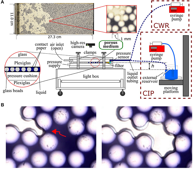
Figure 1. (A) Diagram of the experimental setup, see text. The liquid outlet on the right is connected to one of the modules shown in the dashed squares, depending on the choice of the boundary condition (controlled imposed pressure—CIP, or controlled withdrawal rate—CWR). In the CWR case, the outlet is just connected to the syringe in the pump, and in the CIP case, it is connected to the external reservoir placed above the moving platform. On the top we show a typical image of the experiment and a detailed zoomed in section showing the structure of the porous network, the invading air phase (white) and the defending liquid phase (blue). (B) A typical pore invasion event, imaged with a macro lens. Air invades the defending liquid through the widest pore-throat available to the liquid-air interface at that time (marked by the red arrow on the left image). After the invasion, a new set of pore-throats becomes available to the interface. Adapted from Moura et al. [23] under the Creative Commons CCBY license.

In each experiment, air (non-wetting phase) invades the porous medium from the inlet channel, thus displacing the liquid (wetting phase) previously filling the pore spaces. Since in our experiments the non-wetting phase is the invading phase, we call them drainage experiments (in opposition to imbibition experiments in which the wetting phase invades the medium). Figure 1B shows a typical pore invasion event (imaged with a macro lens to enhance details). The invasion of a given pore happens when the capillary pressure p_c, i.e., the pressure difference between the non-wetting and wetting phases, p_c = p_nw − p_w, is high enough to overcome the capillary pressure threshold $p_c^t$ associated with the geometry of the pore-throat giving access to that specific pore. Narrower pore-throats present higher values of capillary pressure threshold in accordance to the Young-Laplace equation [31], and are, therefore, harder to invade. During the dynamics, the capillary pressure builds up until the invasion of the widest pore-throat available to the air-liquid interface happens (the one having the lowest capillary pressure threshold). Once the pore connected to that pore-throat has been invaded, a new set of pore-throats becomes available for invasion and if one (or more) of these throats happens to have sufficiently low values of capillary pressure threshold $p_c^t$, they can also be invaded without further increasing the capillary pressure, giving rise to the characteristic burst dynamics we study [3, 46, 74]. These invasion events are followed by characteristic pulses in the measured pressure signal, having a typical relaxation signature which is nearly linear in time, for the CWR boundary condition, or exponential, for the CIP boundary condition, as we shall see in details in section 3.3.

The placement of the filter at the outlet boundary allows for the invasion to continue within the model even after breakthrough is achieved, i.e., even after the air phase first percolates through the model, forming a sample spanning cluster. The invasion continues until the moment in which all pores connected to the filter are invaded and the non-wetting fluid saturation reaches its final residual value. We recall that the saturation S of a given phase is understood as the ratio between the volume occupied by that phase in the porous medium and the total pore volume. The placement of the filter allows for a better statistics of the bursts in the vicinity of the outlet region, since the burst count in that area would be much reduced in the case without the filter in which the invasion stops once breakthrough is achieved. Next we move on to the description of the different boundary conditions driving the flow.

2.2. Description of the Boundary Conditions

Two distinct kinds of boundary conditions were used to drive the dynamics of the flow. We will call them controlled withdrawal rate (CWR) and controlled imposed pressure (CIP) boundary conditions. In this section we will describe them, starting from the latter.

2.2.1. Controlled Imposed Pressure (CIP)

The controlled imposed pressure (CIP) boundary condition was designed in order to drive the fluid invasion in a quasi-static manner such that the system would evolve from one equilibrium configuration to another in a slow, controlled fashion. In order to achieve that, the pressure difference across the model had to be dynamically controlled in such a way that it would be just enough to drive the invasion, but not exceedingly high. Had the imposed pressure difference been too high, the invasion would happen fast, and unwanted viscous and inertial effects would be present [75], removing the system from the capillary regime that we propose to study.

We have designed a mechanism composed of an external liquid reservoir (whose detailed description we postpone to Appendix 1 in Supplementary Material) and a logical feedback loop in order to control the pressure difference across the model. The outlet of the system is connected to the liquid reservoir by means of a continuous column of liquid. This reservoir is placed on the top of a moving platform whose height can be electronically set using a step-motor connected to a computer. By controlling the height of the reservoir, one can effectively control the pressure in the liquid phase (the pressure in the air phase is constant and equal to atmospheric pressure since the inlets are kept open in all experiments). The moving platform, liquid reservoir, and an extra syringe pump (whose detailed functionality is described in Appendix 1 in Supplementary Material) form what we call the CIP module, shown in the bottom dashed square on the right of Figure 1A. Once the hydrostatic pressure caused by the height difference h (see Figure 1A) is enough to overcome the minimum value of capillary pressure threshold associated with the line of pores-throats at the inlet, i.e., once $\rho gh>min(p_c^t)$ where g is the gravitational acceleration, the dynamics is triggered and the pore associated with the throat having the lowest capillary pressure threshold $p_c^t$ is invaded. The liquid-air interface has now access to a set of new pore-throats, and if their values of $p_c^t$ are low enough (i.e., if they are wide enough) the invasion progresses until the moment in which all pore-throats available to the interface have capillary pressure thresholds higher than the imposed capillary pressure, i.e., until the condition $p_c^t>\rho gh$ holds true for all available pore-throats. At this moment we say that the system has reached an equilibrium configuration and one has to increase the imposed capillary pressure by lowering again the position of the liquid reservoir (thus increasing the height difference h and the imposed capillary pressure p_c = ρgh) up to the moment in which the invasion starts again. We define a burst in the CIP driven system as any connected set of pores and pore-throats invaded between two time instants in which the imposed capillary pressure had to be increased.

The invasion dynamics is characterized by intervals of inactivity punctuated by localized burst events. This stick-slip process repeats itself throughout the experiment and it would be unpractical (and also very prone to errors) to keep a manual control of the imposed capillary pressure (the external reservoir height). In order to tackle this issue, we have devised an image-based logical feedback loop to handle the control. Figure 2 shows a schematic of this feedback loop. The images recorded from the flow are thresholded to isolate the area A of the air phase. If this area is growing, as in the interval I–II in the figure, in which the area goes from A = A₀ to A = A₀ + dA, more pores are being invaded and we keep the imposed capillary pressure at the current level, say p_c = p₀. If, on the other hand, we perceive that the area growth didn't happen for a long enough interval (a bit longer than 1 min in our case), we say the front has reached a stationary configuration and in order to keep driving the dynamics, we increase the capillary pressure to a value p_c = p₀ + dp. This is done by lowering the liquid reservoir by a given value dh related to dp by dp = ρgdh.

FIGURE 2

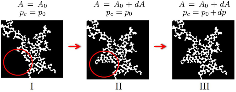
Figure 2. Feedback loop used to drive the CIP experiments. This figure shows a detail from the black and white thresholded image, where the air phase is white and the liquid phase together with the porous medium are black. From I to II, the area of the air phase has grown from A₀ to A₀ + dA, so the capillary pressure is kept constant at p₀ (no change in the liquid reservoir position). From II to III, the area of the air phase does not change, which means the capillary pressure must be increased from p₀ to p₀ + dp (by lowering the liquid reservoir and thus decreasing the pressure in the liquid phase). This analysis is done “on the fly” as the experiment is performed. Adapted from Moura et al. [74] under the Creative Commons CCBY license.

We record images every 15 s during the whole fluid invasion, and the image analysis for the feedback loop is done every 5th image. That means we compare the area of the air phase in, say, the 10th image with that of the 5th in order to decide between the states moving/not moving the liquid reservoir. The amount dh by which the reservoir is lowered is one of our control parameters. During the initial phase of the experiment, the liquid level in the reservoir is at the same height as the porous medium and the system needs to build up a considerable pressure until the invasion starts, therefore, we have chosen a larger dh = dh_max for this initial process and a smaller dh = dh_min to be used after the invasion has started (after the invading phase area reaches a certain small threshold). The values used were dh_max = 100 μm and dh_min = 10 μm corresponding to respective increments in the imposed capillary pressure of approximately dp_max = 1.2 Pa and dp_min = 0.12 Pa. The value of dh was chosen to satisfy the accuracy condition that the height would typically have to be increased several times before new pores are invaded. As long as this condition is satisfied, the results obtained should be independent of the specific value of dh.

One particular point of interest for driving the system under the CIP boundary condition is the fact that in this case the invasion falls into the general class of problems in which an interface moves under the influence of an external (adaptive) force through a medium with quenched disorder. These problems have received a great dose of interest from the scientific community and have been extensively studied theoretically and numerically. Special attention has been paid to the transitions that occur as the external force is increased up to a critical threshold and several scaling relations between the exponents characterizing these critical transitions have been proposed [76, 77]. Our experimental setup thus allows us to directly test the applicability of some of those relations in porous media flows [23].

2.2.2. Controlled Withdrawal Rate

The controlled withdrawal rate (CWR) condition is relatively simpler to implement. Its experimental realization is done by replacing the CIP module in Figure 1A by a syringe pump attached to the model's outlet. There is no need for a feedback loop to control the experiments. In the experiments reported here, we used a constant slow withdrawal rate of q = 0.005 ml/min, thus assuring that the system remains in the capillary regime [5]. The associated capillary number is given by Ca = ρνq/Σγ = 6.1 · 10⁻⁷, where Σ = 1.1 · 10⁻⁴m² is the cross-section of the model. The CWR boundary condition is applied in the majority of two-phase flows studies present in the literature [3, 19, 49, 52]. For the CIP we cannot compute the Capillary number using the same formula, since the flow rate q is not constant. Nevertheless, since the duration of both experiments is similar, we can assume their capillary numbers to be comparable.

When applying a syringe pump to drive the system, one important detail to be considered is the choice between withdrawal of the wetting phase or injection of the non-wetting phase (in the case of drainage studied here). If the compressibility of both phases is negligible, as, for example, in the case of slow displacement of one liquid by another, these two options lead to similar results. Nevertheless, in the case in which one of the phases is compressible, it is preferable to have the syringe pump connected to the other phase, in order to avoid additional effects to the dynamics arising from compressibility (unless those effects are precisely the object of the study, see Jankov et al. [78]). Since air is compressible, we made the choice of having the syringe pump withdrawing the liquid instead.

Another important aspect of this boundary condition is the fact that the liquid displaced from one pore when it is invaded by air cannot immediately leave the system. This happens because the fixed withdrawal rate and typical flux rates during the bursts have very different time scales. In the time scale of a single pore invasion, the volume available for the fluid in the syringe is essentially unaltered. Since the displaced fluid has to go somewhere, it is redistributed to the liquid-air interface in the pore-throats in the vicinity of the invaded pore. This important interface back-contraction effect is responsible for the Haines jumps [53] in the capillary pressure following each pore invasion and has been successfully incorporated into some invasion percolation models to simulate two-phase flow in porous media [3, 19].

3. Results and Discussions

3.1. Dynamics of the Air Saturation

To give an idea of the evolution of an experiment, we show in Figure 3A a sequence of snapshots of the flow (here driven by controlling the imposed pressure—CIP boundary condition). The current time (in hours) and imposed capillary pressure (in Pascals) are shown under each image. The time difference between the first and last images is about 82 h. The air inlet is on the left and the filter is the black stripe on the right. In Figure 3B, we show a spatiotemporal map of the full invasion. The color map gives the invasion time of each pore in the system. Notice that if the outlet filter were not present, the invasion would have stopped at the moment of breakthrough, when the air phase first percolates through the model. This corresponds to t ≈ 60h in Figure 3B. Without the filter, the whole red region in the figure would not have been invaded.

FIGURE 3

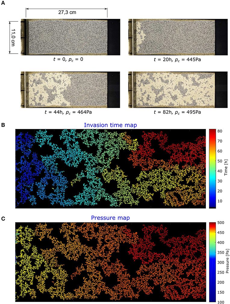
Figure 3. (A) Images from the drainage process driven by the CIP boundary condition. The time t of each image is shown in hours and the instantaneous capillary pressure p_c in Pascal. The porous medium is initially saturated with the liquid phase (blue) which is then gradually displaced by the invading air phase (white). On (B) we show a spatiotemporal map of the invasion, the color code indicating the invasion time of a given pore. On (C) we show the imposed pressure map, in which the color code denotes the imposed pressure (given by the height of the external reservoir), at which the invasion of a given pore occurred.

The spatiotemporal map shown in Figure 3B is a very useful matrix: once this map is computed, one does not need to rely on a large collection of pictures/video any longer. In practice this brings the benefit of dramatically reducing the computational time for any further analysis.

Since we are controlling the imposed pressure (by controlling the level of the external reservoir, see Figure 1A), we can also define a pressure map for the flow, here shown in Figure 3C. The color code (shifted with respect to Figure 3B to aid visualization) indicates the imposed capillary pressure during the invasion of a given pore. Notice that for the system studied here, the majority of the invasion happens in a relatively narrow band of imposed pressures between 420 Pa and 480 Pa.

The box counting fractal dimension [79] of the invading structure was measured to be D = 1.76 ± 0.05 for CIP and D = 1.75 ± 0.05 for CWR, therefore, with respect to the morphology, one can say that both boundary conditions yield similar structures (for similar capillary numbers). Nevertheless, despite these similarities in morphology, there are some very clear differences in the dynamics of the different systems. In particular, the evolution in time of the air phase saturation happens very differently. For the CWR, since the withdrawal rate of the liquid is constant, externally set by the syringe pump, we expect the area growth of the air phase to happen linearly, in a steady controlled manner, following the same rate of the imposed withdrawing. This behavior is observed in Figure 4, where the phase saturation is determined directly from the images of the flow. The red curve (bottom) shows the data for the CWR case. We see that once the invasion starts, it progresses at the constant rate imposed by the syringe pump. Conversely, for the CIP boundary condition, the air saturation evolution happens in a much more intermittent fashion, in which intervals of stagnation are followed by periods of sudden growth, as shown in the blue curve (top) in Figure 4 and more clearly in the zoomed-in inset. These differences in the dynamics of invasion will be reflected later in the power spectral density of the pressure signal, to be analyzed in section 3.5.

FIGURE 4

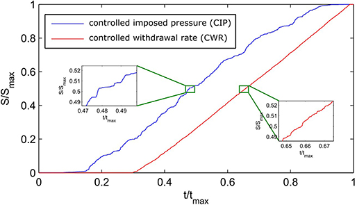
Figure 4. Temporal growth of the air saturation measured from the area of the invading air phase (same model shown in Figure 3). Time and saturation are normalized by their final values, t_max and S_max, respectively. The blue curve (top) shows the data for the controlled imposed pressure (CIP) boundary condition, whereas the red one (bottom) is for the controlled withdrawal rate (CWR). As expected, the later shows a rather constant growth rate, set from the external syringe pump. For the CIP case, we see a much different scenario, with intervals of relative stagnation being followed by periods of sudden area growth in an intermittent manner. The zoomed-in insets emphasize this difference.

3.2. Geometrical Characterization of the CIP Bursts

Our setup allows us to directly visualize the invasion bursts from the images of the flow. Let us consider the experiment shown in Figure 3 in which the system is driven under the CIP boundary condition. In an ideal scenario, with infinite precision, once the system reaches an equilibrium state, i.e., one at which the imposed pressure difference is not enough to invade any of the pore-throats available to the liquid-air interface, we would like to be able to increase the pressure difference ever so slightly to trigger the invasion through one and only one of the pore-throats (the widest among the ones available to the liquid-air interface). A burst could then be naturally defined as the region that is invaded following the invasion of this particular pore-throat until the interface reaches a configuration in which again all pore-throats available are too narrow to be invaded and the imposed capillary pressure has to be increased once again. This burst's size would be given by the number of invaded pores and the burst's duration Θ could be identified as the time interval between the two instants at which the imposed pressure was increased (immediately before and after the burst). With our current setup, with pressure increments of the order of dp_min = 0.12 Pa, we still don't get to that idealized level of accuracy and very frequently, after increasing the pressure, the invasion is triggered from a small number of pore-throats (between 3 and 4 on average). We therefore consider the connected invasion starting from each of these pore-throats as separate bursts, all of which are associated to the same time interval Θ. Our definition of bursts for the CIP experiments is then the connected set of pores that have been invaded from a given pore-throat until the imposed pressure needs to be again increased. Notice that this definition makes explicit use of the fact that the bursts happen at constant imposed pressure, therefore, it is only suitable for the CIP case.

Figure 5 shows the resulting bursts. In the top part of the figure, they are colored by their area, normalized by a characteristic pore area (100 pixels ≈ 0.3 mm² in these images). In the bottom part of the figure, the same bursts are shown with random coloring, in order to emphasize their individual shapes. Notice that the vast blue areas in the top image are indeed formed by a large number of small bursts (see the detail in the images). Only bursts having their centroids lying in the central 90% of the model's length are considered, in order to avoid possible boundary effects which have been observed to happen in the vicinity of the inlet and outlet of the flow [74].

FIGURE 5

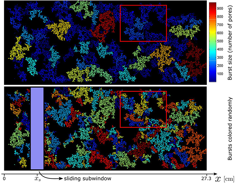
Figure 5. Invasion until final saturation for the CIP boundary condition, using the same model shown in Figure 3. (Top) Individual bursts color coded by their size, computed dividing the burst area by the characteristic pore area of 100 pixels ≈ 3 mm. (Bottom) Individual bursts color coded randomly, to allow the visualization of separate bursts of similar size. Notice in particular that the vast blue areas in the top image are indeed formed by a set of smaller bursts, as can be seen in the detail (red rectangle). The sliding subwindow centered at x_s is used in connection with the spatial distribution of bursts. In both images, only bursts with centroids lying in the central 90% of the model's length are shown. Adapted from Moura et al. [23] under the Creative Commons CCBY license.

The experimental assessment of individual bursts provided in Figure 5 yields a valuable amount of information about the dynamics. It has been shown [23] that the distribution N(n) of bursts of size n (where n is the estimated number of pores, computed by normalizing the burst area by a typical pore area) follows the scaling N(n) ∝ n^−τ, where τ = 1.37 ± 0.05. The burst dynamics is therefore self-similar, having no characteristic intrinsic length scale [80]. The exponent τ measured is consistent with the theoretical value τ = 1.30 ± 0.05 predicted by numerical simulations (invasion percolation) and analytical results [23, 45, 76, 81].

From Figure 5 one cannot directly notice any tendency of concentration of larger bursts toward one of the ends of the model. Indeed, the amount of bursts and their average sizes seem to be approximately homogeneously distributed along the system's length. In order to validate this statement quantitatively, we have analyzed the average burst size ${\bar{n}}_s$ (burst area divided by typical pore area ≈ 3 mm.) and the total number of bursts ξ_s within sliding subwindows having a fixed length of 2 cm and width spanning the whole width of the model, see Figure 5. For each subwindow, we have computed the number of bursts ξ_s whose centroid lie inside it and their corresponding average bursts size ${\bar{n}}_s$. The results are shown in Figure 6A. The correlation observed between consecutive measurements arises from the fact that neighboring subwindows overlap: the centers of consecutive subwindows are separated by 0.2 cm, whereas the subwindow length is 2 cm, thus yielding 90% overlap between neighboring subwindows. From the analysis of this figure, we cannot observe any systematic trend for the average size or number of bursts: when seen separately, neither of the average burst size nor the number of bursts seem to be systematically increasing or decreasing with the subwindow position. Nevertheless, when comparing one against the other, we can observe a clear anti-correlation of the data. This anti-correlation is confirmed by measuring the Pearson's correlation coefficient, given by

FIGURE 6

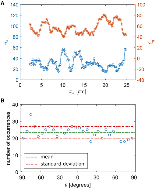
Figure 6. (A) Average burst size ${\bar{n}}_s$ (bottom curve, left scale) and number of bursts ξ_s (top curve, right scale) inside sliding subwindows centered at x_s (see Figure 5). The sliding subwindow spans the whole width of the system and has a fixed length of 2 cm. The spatial distribution of bursts follows no systematic trend along the model. The average burst size ${\bar{n}}_s$ is computed by dividing the burst area by typical pore area ≈ 3 mm. (B) Histogram showing the random orientation of the bursts shown in Figure 5. The thicker green line shows the mean of the distribution and the thinner red lines show its standard deviation.

$\begin{array}{ll}\rho =\frac{\frac{1}{N}{\displaystyle {\sum }_{i=1}^N}\left({\bar{n}}_{s_i}-\langle {\bar{n}}_s\rangle \right)\left({\xi }_{s_i}-\langle {\xi }_s\rangle \right)}{{\sigma }_{{\bar{n}}_s}{\sigma }_{{\xi }_s}}=-0.68,& (1)\end{array}$

where ${\bar{n}}_{s_i}$ and ξ_si correspond respectively to the values of the average burst size and number of bursts inside the ith subwindow (i = 1, 2…N), 〈.〉 denotes averaging and ${\sigma }_{{\bar{n}}_s}$ and σ_ξs are the standard deviations of the respective quantities. Since the Pearson's coefficient is negative, the average burst size ${\bar{n}}_s$ and number of bursts ξ_s measured in a sliding subwindow are anti-correlated. The origin of this anti-correlation is easily understood: if the system is in a steady regime, the total invaded area in a subwindow is approximately constant (apart from statistical fluctuations arising from the randomness of the porous medium and the underlying dynamics [74]). The products of the two quantities, average burst size ${\bar{n}}_s$ and the number of bursts ξ_s inside a subwindow, gives the total area of bursts having centroid inside that subwindow. This is not exactly equal to the total invaded area A_s inside the subwindow, since the boundaries of the bursts (particularly the larger ones) could cross the imaginary subwindow boundary, but it gives an approximation to it. Therefore, one can expect the product between the average burst size and the number of bursts inside a subwindow to be approximately constant over the length of the model (apart from statistical fluctuations), thus yielding the observed anti-correlation:

$\begin{array}{ll}{\bar{n}}_s{\xi }_s\approx A_s\approx cte.& (2)\end{array}$

As mentioned previously, the dynamics of our drainage experiments happen in the capillary regime [3, 5], i.e., it is governed primarily by capillary forces. Since the pore-size distribution is nearly isotropic, due to the construction routine employed to make the models in which the glass beads are randomly placed, the capillary forces involved should also be isotropically distributed. We expect this property to be translated into the dynamics, generating bursts with no privileged direction within the model. One can have a qualitative picture of this statement directly from Figure 5 and a more quantitative result can be obtained by producing a histogram of the bursts orientation angle θ. This angle is defined as the one between the x-axis (inlet–outlet direction, see Figure 5) and the major axis of an ellipse having the same second-moments as that particular burst. Figure 6B shows the resulting histogram. We can see that, apart from fluctuations caused by the small size of the dataset, there isn't any particularly privileged orientation for the bursts. Indeed, such a distribution also indicates that viscous effects are much reduced in the experiment: if the dynamics were driven by viscous forces, one would observe bursts much more elongated in the inlet–outlet direction, following the average gradient of pressure in that direction. A distribution of burst angles would not be isotropic, but show a peak toward smaller angles and a corresponding reduction for larger angles.

Up to this moment, we have concentrated our analysis mostly on quantities that could be obtained from the images of the flow. In the coming sections, we will shift our focus to the analysis of the pressure measurements, for both boundary conditions. We begin by briefly analyzing the typical signature of the measured pressure signal during the invasion.

3.3. Typical Signature of the Pressure Measurements

As anticipated, in spite of having nearly indistinguishable large-scale morphology, the dynamical features of the invasion differ considerably between the CIP and CWR boundary conditions. This difference is clearly observable in the evolution of the measured pressure signal, as shown in Figure 7. Let us focus initially on the CWR signal in Figure 7A. Clear pulses in the capillary pressure corresponding to the pore-invasion events are observed (also termed Haines jumps [53]). Each pulse is composed of one drop phase and one relaxation phase (see arrows in the figure). Morrow [82] has used the terms rheon and ison to describe drop and relaxation phases respectively. The pressure drops correspond to the moments in which one or more pores are invaded and the liquid volume that previously filled them is redistributed to the menisci in the surrounding pore-throats (see Figure 1B). The slower relaxation part corresponds to the moments in which the menisci of the air-liquid interface slowly advance inside the pore-throat, as a response to the constant withdrawal rate imposed by the external syringe pump. The capillary pressure slowly increases, as the menisci reach narrower parts of the pore-throat up to the moment when the pressure threshold associated to the widest pore-throat is reached, the interface then becomes unstable and a new pore-invasion occurs, giving rise to another pressure drop [3].

FIGURE 7

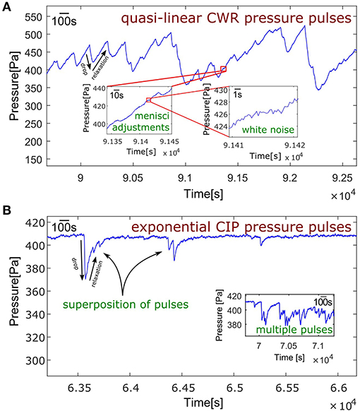
Figure 7. Typical pressure signal signatures for experiments performed under different boundary conditions. The signals are formed by a sequence of pulses, each formed by one drop and one relaxation phase. During the drop phase one or several pores are invaded. During the relaxation phase the capillary pressure increases again as the menisci readjust themselves inside the pore-throats, see arrows. (A) For the CWR boundary conditions, the signal presents a quasi-linear relaxation behavior. The pressure pulses themselves are seen in the larger scale, while menisci readjustments and the white noise from the sensor are shown in the respective insets. (B) For the CIP boundary condition, the pulses happen in an intermittent fashion. Long intervals of inactivity are punctuated by sudden events and the relaxation behavior has an exponential signature in which the capillary pressure relaxes back to the level imposed by the external liquid reservoir. A pressure pulse can trigger others and even give rise to a large avalanche composed of multiple pulses.

The connection between the capillary pressure and the volume of liquid redistributed to (drop phase) or withdrawn from the interface (relaxation phase) was explored in Måløy et al. [3] by introducing the concept of a capacitive volume κ such that dV_p = κdp_c, where dV_p is the liquid volume displaced from an interface pore throat in response to a change dp_c in capillary pressure. The volume dV_p can be connected to the total volume dV redistributed to or withdrawn from the whole interface as dV_p = dV/n_f, where n_f is the number of pore-throats belonging to the liquid-air interface. By putting these pieces together we get

$\begin{array}{ll}d{p}_c=\frac{dV}{\kappa n_f}.& (3)\end{array}$

Considering that the process occurs in a time dt, we have that the variation dp_c/dt is connected to the total flux q_i = dV/dt by

$\begin{array}{ll}\frac{d{p}_c}{dt}=\frac{q_i}{\kappa n_f},& (4)\end{array}$

where q_i = q_R for the relaxation phase and q_i = q_D for the drop phase. During the relaxation phase the flux q_R withdrawn from the interface, matches the externally imposed withdrawal flux (q_R = q = 0.005ml/min in our case). For the drop phase the flux q_D redistributed to the interface can be estimated as $q_D=n_f{a}^2{v}_b$, where v_b is a characteristic back-contraction velocity of the interface. Like the Darcy velocity [1], v_b is expected to vary inversely with the viscosity of the fluid. So for experiments conducted with a less viscous fluid, one would expect a higher v_b which leads to a higher redistribution flux q_D during the drop phase and consequentially a steeper pressure drop in accordance with Equation (4). Indeed this can be seen when comparing the drop phase of our experiment in Figure 7A (where a high-viscosity liquid was used) against the pressure signal of an experiment in which water is used, like in Figure 1D in Måløy et al. [3] for example. Notice that in the figure in Måløy et al. [3], the vertical axis denotes the pressure in the liquid phase, while in our case we show the capillary pressure instead, i.e., the difference between the pressure in the air and liquid phase. So the downwards drops in Figure 7A are to be compared against the steeper upward sections of the signal in Måløy et al. [3]. While q_R is an externally imposed parameter, q_D is to be understood as an intrinsic parameter, dependent on the viscosity of the wetting phase.

Notice that the inverse dependence of the capillary pressure drop with the number of pore-throats in the system shown in Equation (3) implies that the existence of the pressure drops (Haines jumps) is a direct consequence of the finite size of the system. For a large enough system(n_f → ∞), the pressure jumps cease to exist [3].

If one zooms further in one of the relaxation phases, one can observe (left inset in Figure 7A) some low amplitude fluctuations in the signal, corresponding to small adjustments of the menisci inside the pore-throats that happen before the invasion of another pore. Such adjustments are not easily observable from our images, since they happen at very short time and length scales. Nevertheless, they are bound to occur in any case of slow flow in a porous medium (both in drainage and imbibition). Zooming even further in on the signal allows one to see the high frequency random fluctuations (right inset in Figure 7A) which are expected from any electronic measuring device, in our case the pressure sensor employed. These fluctuations set the error in the pressure measurements to be on the order of δp = 0.5 Pa.

For the CIP boundary condition, shown in Figure 7B, we see that the pressure signal presents an entirely different signature. Most of the time the system is in a stagnation state, in which the capillary pressure, set by the external reservoir position, is (very slowly) increased. This corresponds to the nearly horizontal level approximately at 405 Pa in Figure 7B. Those large intervals of stagnation are punctuated by sudden activity events, seen as the nearly vertical drops followed by the exponential relaxation phases in the figure. Energy is slowly fed into the system during stagnation periods between pore invasion events and is rapidly released (and further dissipated by viscosity) during the fast invasion events. Differently from the CWR, in the CIP case the pressure pulses present a nearly exponential relaxation behavior. One pulse can eventually trigger others or even give rise to a large avalanche of multiple pressure pulses, as seen in the inset of Figure 7B.

In the CWR system, the total available liquid volume in the experiment is composed by the volumes of (a) the liquid phase in the porous medium, (b) the volume inside the tubing connected to the outlet and (c) the (slowly changing) volume of the syringe pump. Once a pore is invaded by air, the liquid volume previously filling that pore has to be redistributed to the liquid-air interface in the pore-throats in the vicinity of that pore because the time scale needed for the pump to buildup that extra volume in the syringe outside the medium is much larger than the typical time scale of a burst. On the other hand, when the system is driven under the CIP boundary condition, after a pore invasion, the interface back-contraction is much reduced, since the liquid previously filling the pore can freely flow outside of the system and into the pressure reservoir (see Figure 1A). This difference in boundary condition is ultimately responsible for the nearly exponential relaxation behavior shown in the CIP case. A full derivation of this behavior was done in Moura et al. [23] and we include it here in Appendix 2 in Supplementary Material.

The differences in the pressure signatures is further reflected on the signal's power spectral density, as we shall see in section 3.5. In the following section we will perform an analysis of time-directed avalanches in the CWR pressure signal.

3.4. Avalanches in the CWR Pressure Signal

In this section we will give a statistical characterization of the pressure signal for the CWR experiments by considering the concept of time-directed avalanches. This concept was previously used in numerical simulations by Roux and Guyon [72] and Maslov [83] and in both simulations and experiments by Aker et al. [84] and Biswas et al. [85]. Figure 8A shows the full pressure signal and a zoomed in section is seen in Figure 8B. The forward time-directed avalanches are presented as the green horizontal lines, black dots denote the set of local maxima of the signal (starting points for the avalanches) and the red crosses correspond to the local minima of the signal. Each forward avalanche corresponds to the time interval T_f between the moment at which a pressure drop starts and the first moment at which the pressure reaches a level equal to that from the starting point (in the future with respect to the starting time). Conversely, a backward avalanche can be defined as the time interval T_b between a local maximum (again one of the black dots) and the last moment at which the pressure reached a level equal to that from the starting point (in the past with respect to the starting time). Backward avalanches can be computed simply as forward avalanches in the time-reversed pressure signal. We have included in Figure 8B one arrowed green line to denote a forward avalanche of size T_f and one arrowed purple line to denote a backward avalanche of size T_b.

FIGURE 8

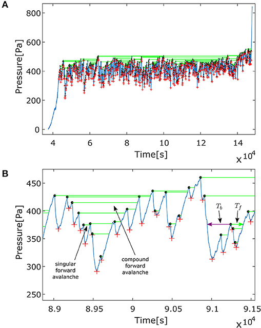
Figure 8. (A) Full Pressure signal from the CWR experiment, black dots and red crosses denote the local maxima and minima of the signal. The forward avalanches are denoted by the green horizontal lines. (B) A zoomed segment of the signal. The sizes T_f and T_b of forward (green arrow) and backward avalanches (purple arrow) are shown for a particular starting point. Examples of singular and compound forward avalanches are also shown.

Notice that the definition of time-directed avalanches employed here has a hierarchical structure: a particular avalanche can encompass a number n of others. Each avalanche defines a “pressure valley,” the region of the pressure signal between the beginning and end of the avalanche. Each valley is composed of either one (in the case of a singular avalanche) or a series of pressure drops (compound avalanche) each drop corresponding to a pressure difference $\Delta p_i^D$ (difference between the pressure level of a black point and the following red point in Figure 8B). The forward valley size χ_f is defined as the sum of all the pressure drops within the valley, i.e.,

$\begin{array}{ll}{\chi }_f={\displaystyle \sum _{i=1}^n}\Delta p_i^D.& (5)\end{array}$

Backward valley sizes can be defined in an analogous manner.

For each avalanche of size T_f, we can then measure the respective valley size χ_f. In Figure 9 we show a scatter plot between the two quantities for all forward avalanches (singular and compound) in the experiment. We observe that there is a clear correlation between the quantities, i.e., χ_f ∝ T_f. The Pearson's correlation coefficient was measured to be ρ = 0.995.

FIGURE 9

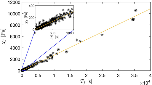
Figure 9. Correlation between the avalanche size T_f (in seconds), and the respective valley size χ_f (in Pascals). The Pearson's correlation coefficient was measured to be ρ = 0.995.

This correlation is not accidental and can be easily understood. Let us assume that the derivatives of the pressure signal in the drop and relaxation phases are approximately constant, given by Equation (4). Notice that during a given avalanche, the pressure goes down a number n of times and the total time spent in these drop phases is given simply by $T_f^D=\sum \Delta p_i^D/|d{p}_c/dt|$. A similar expression can be derived for the total time spent on the relaxation phases for a given avalanche, i.e., $T_f^R=\sum \Delta p_i^R/|d{p}_c/dt|$, where $\Delta p_i^R$ denote the increments in pressure. Notice that the time derivative of the pressure signal is different for each phase, in accordance to Equation (4). Notice also that although the consecutive pressure differences associated with the drop and relaxation phases are not necessarily equal, the sum of all the pressure drops during an avalanche equals the sum of all pressure increments, i.e., $\sum \Delta p_i^R=\sum \Delta p_i^D={\chi }_f$. The reason for that is the fact that subtracting all the increments from all the drops in pressure equals zero for any avalanche, since the end point of an avalanche has, by definition, the same pressure as the starting point (same height in Figure 8B). To put it differently, the cumulative lowering in capillary pressure equals the cumulative increments for any given avalanche, since the pressure at the end equals that of the beginning of the avalanche.

Using again Equation (4), we have that the total time spent in the drop phases for a given avalanche equals $T_f^D=\kappa n_f{\chi }_f/q_D$. Similarly, for the relaxation phases, we have $T_f^R=\kappa n_f{\chi }_f/q_R$. The total avalanche time $T_f=T_f^D+T_f^R$, i.e.,

$\begin{array}{ll}{T}_f=\kappa n_f\left(\frac{1}{q_D}+\frac{1}{q_R}\right){\chi }_f,& (6)\end{array}$

where q_D and q_R are respectively the volumetric fluid flux given to the interface during the drop phase and withdrawn from it during the relaxation phase. Notice that when using Equation (4) to obtain Equation (6), we have assumed the linearity relation between the pressure drop and the fluid volume given to (drop phase) or withdrawn from the interface (relaxation phase), as expressed in Equation (3).

Equation (6) shows a neat connection between statistical quantities defined over the pressure signal (the avalanche size T_f and valley size χ_f), the current state of the invasion (via the size of the invasion front n_f), an externally imposed control parameter (the flow rate q_R which here matches the external syringe flow rate q) and intrinsic properties of the system (the capacitive volume κ and the flow rate q_D, the later depending inversely on the viscosity of the wetting phase).

Next we analyze the size distribution of forward avalanches N_all(T_f). For convenience, we will use the same notation N_all(X) to denote the distribution of any quantity X. The subscript indicates that one counts all avalanches (singular and compound). The distribution N_all(T_f) is shown in Figure 10A. We have measured the scaling $N_{all}(T_f)\propto T_f^{-{\tau }_{all}}$, with τ_all = 1.67 ± 0.05 over times ranging from 100s (the typical duration of a short singular avalanche in our experiment, see Figure 8B), to around 20000s corresponding to a large compound avalanche. In the inset of the figure we present a scatter plot showing the correlation between the avalanche size and the number of sub-avalanches within it. As anticipated, larger avalanches are typically composed of a larger number of sub-avalanches, as we see in the plot. The measured Pearson's correlation coefficient was ρ = 0.998.

FIGURE 10

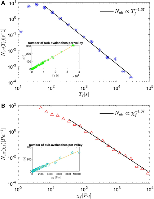
Figure 10. (A) Distribution of forward time-directed avalanches. The black line denotes the scaling $N_{all}(T_f)\propto T_f^{-1.67}$. In the inset we present a scatter plot illustrating the correlation between the avalanche size T_f (in seconds) and the number n of sub-avalanches within it. The measured Pearson coefficient was 0.998. (B) Distribution of forward valley sizes. The black line denotes the scaling $N_{all}({\chi }_f)\propto {\chi }_f^{-1.67}$. In the inset we present a scatter plot illustrating the correlation between the valley size χ_f (in Pa) and the number n of sub-avalanches within it. The measured Pearson coefficient was 0.994.

The scaling exponent for the distribution N_all(T_f) measured here differs from value τ_all = 1.9 ± 0.1 reported in Aker et al. [84]. It also differs from the superuniversal theoretical prediction τ_all = 2 for invasion percolation and a number of other growth models presented in Maslov [83]. There are a number of factors behind this difference. First, the standard invasion percolation algorithm does not include effects from viscous dissipation and the back-contraction of the liquid-air interface after each pore invasion, present in the experimental case. Additionally, the pore structure of our models is not entirely uncorrelated. Some degree of correlation must exist due to the technique employed in the model construction. As previously explained, the setup is constructed by letting the glass beads fall onto the sticky side of a contact paper sheet. If the glass beads were mathematical points without dimension, randomly placing them in the contact paper should ideally generate an uncorrelated structure, but this is not the case when the beads have a finite size (1mm diameter in our case) and cannot physically overlap. In a recent study, Biswas et al. [85] have shown that indeed very little correlation in the pore structure can lead to changes in the critical exponents associated with the invasion process. The authors have shown in particular that the forward avalanches exponent does not need to assume the superuniversal value τ_all = 2. Indeed, using numerical simulations Biswas et al. have shown that the forward avalanche exponent assumes the value τ_all = 1.66 ± 0.04 for correlated porous samples, which is in direct agreement with our measurements presented in Figure 10A. When the simulations were performed in an uncorrelated porous medium, the authors have measured the exponent τ_all = 1.99 ± 0.05, in agreement with the theoretical predictions in Maslov [83].

As an additional check of our results, we have measured the valley sizes distribution N_all(χ_f). Since the quantities T_f and χ_f are clearly correlated (as seen in Figure 9), the distribution N_all(χ_f) should present the same scaling behavior as N_all(T_f). Indeed this is what we observe, see Figure 10B where the black line denotes the scaling ${\chi }_f^{-{\tau }_{all}}$, with τ_all = 1.67 ± 0.05. In the inset we show the scatter plot between the valley size χ_f and the number n of sub-avalanches inside it. Not surprisingly, we find that χ_f ∝ n since it had previously been shown that T_f ∝ n and χ_f ∝ T_f (Figures 9, 10A).

There's an important technical point about the computation of the avalanches employed here. As previously seen, it requires finding the local maxima and minima in the pressure signal as an initial step. In a smooth signal, this can be done easily by simply finding the points where the first derivative of the time series changes from positive to negative for the local maxima and vice-versa for the minima. But in a natural noisy signal, this approach is problematic due to high frequency fluctuations. One possible way to handle the issue is by employing a low-pass filter to remove the high frequency noise. This was our initial approach but it led to biases in the statistics, particularly in the region of small valley sizes. We decided to avoid the filter completely and perform the analysis in the raw signal employing a different technique to find the local extrema. We have employed Matlab's findpeaks routine to find all maxima in the noisy data and sort them out with respect to the peak prominence (a measure of the distance between the top of a particular peak and the surrounding signal). This can be used to remove most of the peaks mistakenly assigned to the fluctuations because they are very small. Next, we have excluded from the data all peaks that were followed by a pressure drop smaller than a certain small threshold, which we have arbitrarily chosen to be Δp^D = 4 Pa. This threshold is chosen arbitrarily, but we have checked that all exponents of the distributions reported here did not vary significantly for any value in the interval 2 Pa < Δp^D < 6 Pa.

For completeness we also include the distribution of backward avalanches T_b and valley sizes χ_b. These are found in Figures 11A,B, respectively. The insets show the correlations between T_b and n in (a) and χ_b and n in (b), where n denotes again the number of sub-avalanches. Interestingly the distributions of T_b and χ_b seem to present a crossover behavior, where the small avalanches scaling show an exponent that is smaller than the one for the large avalanches. We have measured the scaling exponent τ_allb = 1.55 ± 0.05 for avalanches larger than a given crossover scale and τ_allb = 0.90 ± 0.08 for avalanches smaller than this scale. The existence of a very similar crossover behavior had been reported in simulations performed in Biswas et al. [85], where the authors explained that small avalanches are influenced by effects coming from the local correlations in the pore structure. Larger avalanches on the other hand, being averaged over many pores, do not feel such local correlations. Our experiments are in direct agreement with the exponents reported in Biswas et al. [85], where it was measured τ_allb = 1.59 ± 0.06 for the larger avalanches and τ_allb = 0.93 ± 0.03 for the smaller ones.

FIGURE 11

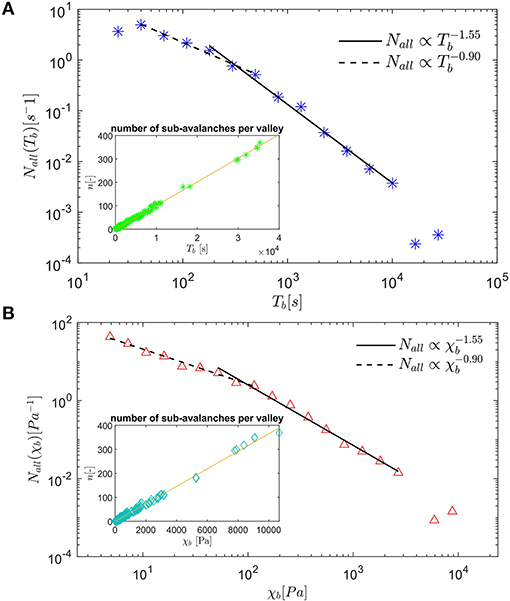
Figure 11. (A) Distribution of backward time-directed avalanches. The black line denotes the scaling $N_{all}(T_b)\propto T_b^{-1.55}$ and the dashed line corresponds to $N_{all}(T_b)\propto T_b^{-0.90}$. In the inset we present a scatter plot between the backward avalanche size T_b (in seconds) and the number n of sub-avalanches within it. The measured Pearson coefficient was 0.998. (B) Similar distributions for the backward valley sizes, the black line corresponds to $N_{all}({\chi }_b)\propto {\chi }_b^{-1.55}$ and the dashed line to $N_{all}({\chi }_b)\propto {\chi }_b^{-0.90}$. In the inset we present a scatter plot between the backward valley size χ_b (in Pa) and the number n of sub-avalanches within it. The measured Pearson coefficient was 0.997.

The distribution of starting pressures (black dots in Figure 8) for the avalanches can also be directly obtained from our data. It is shown in Figure 12. Notice that, the majority of the avalanches have starting points in the interval between 420 Pa and 480 Pa. This is in line with what we had previously observed in the CIP case (Figure 3C). The measurement in Figure 12 is also similar to what was found for an experiment performed in a similar model with different fluids in Furuberg et al. [19].

FIGURE 12

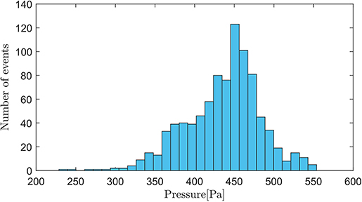
Figure 12. Distribution of avalanches starting pressures (black dots in Figure 8).

Next we move on to the analysis of the power spectral density of the pressure signals. The analysis presented here includes and extends the work initiated in Moura et al. [24].

3.5. Power Spectral Density of the Pressure Signal

The different temporal signatures for the CWR and CIP pressure bursts are translated into the power spectral density (PSD) of the signal. Figure 13 shows the PSD S = S(f) for the CWR (red dots) and CIP (green crosses) boundary conditions, the later being shifted upwards 4 orders of magnitude to aid visualization. Both PSDs present a scaling behavior S ∝ f^−α, with two apparent crossover regions. We show in Figure 13 a set of guide-to-eye lines with the respective slopes for each scaling regime. Let us focus initially on the CWR case. In order to analyze each of these scaling regions separately, let us look again at the typical signature of the pressure signal for the CWR experiment, shown in Figure 7A. On the larger scale, we see the characteristic pulses in pressure, each of which is caused by the geometrical invasion of one or more pores by the air phase. Those pulses happen at intervals that match the period range of the first scaling regime in the PSD (α = 1.5 for frequency f in the approximate interval [0.001, 0.005 Hz], with corresponding periods T in the range [200, 1,000 s]), which indicate that their presence is responsible for this scaling regime. If we zoom into that scale, we see (inset on the left in Figure 7A) that there are some oscillations of the pressure signal happening in the phase of pressure build up that precedes the bursts. These happen with typical periods in the range corresponding to the second scaling regime (α = 3.5 for f in [0.007, 0.018 Hz] and corresponding T in [50, 140 s]). We believe those pressure oscillations are related to tiny adjustments of the air-liquid front, happening in between burst events while the front is in a stable position, as previously stated. Such adjustments are not easily observable from our images, since they happen at very short time and length scales. Finally, if we zoom in even further on the signal, we see (inset on the right in Figure 7A) the typical high frequency random fluctuations expected from any electronic measuring device. In the case of our pressure sensor, they are on the order of 0.5 Pa and, as expected, lead to the high frequency white noise region of the PSD, the plateau on the right of Figure 13 (α = 0 for f in [0.5, 1.76 Hz] and corresponding T in [0.5, 2 s]). The highest frequency in the graph is the Nyquist frequency, f_N = 1.76 Hz, which corresponds to half of the acquisition frequency employed in that particular CWR experiment. Notice also that there is a single isolated point in the very low frequency part of the PSD (extreme left in Figure 13) that falls far from the scaling region. This point is present in all experiments and is not an outlier in the data: its existence signals the very slow positive drift in the pressure signal, which occurs since the capillary pressure has to increase (albeit very slowly after the front reaches a propagating regime [74]) in order to give access to the invasion of narrower pores as the front progresses inside the medium.

FIGURE 13

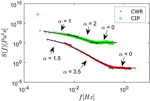
Figure 13. Power spectral density of the pressure signal for CWR (red dots) and CIP (green crosses) boundary conditions, the later being shifted upwards 4 orders of magnitude. Both systems present scaling behavior for the PSD of the form S ∝ f^−α, with different exponents α shown by the guide-to-eye lines. In both cases, the spectra for high frequencies present the typical flat profile characteristic of white noise from the experimental measuring device. Notice that for the CIP case, a region consistent with 1/f scaling (pink noise) for the low-frequency events is observed, followed by a 1/f² (brown noise) region for intermediate frequencies.

Next, let us move to the analysis of the pressure signal associated to the CIP boundary condition. As previously mentioned, the CIP pressure pulses look very different from the ones associated to the CWR case. They are composed of a sudden drop followed by a nearly exponential relaxation behavior, which is rather different from the signature shown for the CWR case (see Figure 7). This difference is reflected in the power spectral density for the CIP case, shown in green (crosses) in Figure 13. We notice that once again the PSD presents the scaling S ∝ f^−α with three characteristic scaling regimes, but this time with exponents α = 1 (pink noise) for the lower frequencies, α = 2 (brown noise) for intermediate frequencies and again α = 0 (white noise) for the higher frequencies. As earlier, the lines shown in the plot are to be understood only as guide-to-eye lines and not as accurate measurements of the exponents (which would require data extending for a longer range of time/frequency scales). The scaling region related to the bursts now has exponent α = 1 (1/f noise, also known as pink noise). The appearance of 1/f noise and the following crossing over to 1/f² scaling is an interesting observation, which has been noticed in a number of other systems, including in the very first reported observation of 1/f noise [86] (flicker noise in vacuum tubes).

In the following section we present a fully integrable mathematical framework that can be used to explain the unusual scaling behavior observed for the CIP boundary condition. This framework is an generalization of the one presented in Moura et al. [23]. A similar framework for the CWR case is still lacking.

3.6. Analytical Model for the 1/f to 1/f² Transition in the CIP Power Spectral Density

As noted in Figures 7, 13, the pressure signal in the CIP case presents bursts with an exponential relaxation behavior and yields an interesting non-trivial PSD presenting a 1/f to 1/f² transition (pink noise to brown noise transition). In this section we propose an analytical framework to explain this unusual PSD scaling. This framework is an adaptation of an argument proposed in Ziel [87]. A similar argument was also presented by Bernamont [88] and a review can be found in Milotti [89].

Motivated by Figure 7, let us consider that, apart from a nearly constant offset, the pressure signal can be modeled as a train of exponentially decaying pulses located at a set of randomly distributed discrete times t_j

$\begin{array}{ll}{p}_{\lambda }(t)={\displaystyle \sum _j}AH(t-t_j)e^{-\lambda (t-t_j)},& (7)\end{array}$

where λ > 0 and A < 0 are initially assumed to be constants (the characteristic decay rate and amplitude of the pulses) and H(t − t_j) is the Heaviside step function [90], i.e., H(t − t_j) = 0 if t < t_j and H(t − t_j) = 1 if t ≥ t_j. The characteristic decaying time of the pulses is given by t_c = 1/λ. Let P_λ(f) be the Fourier transform of p_λ(t),

$\begin{array}{ll}{P}_{\lambda }(f)={\displaystyle {\int }_{-\infty }^{\infty }}{p}_{\lambda }(t)e^{-i2\pi ft}dt& (8)\end{array}$

$\begin{array}{rr}=A{\displaystyle \sum _j}{e}^{\lambda t_j}{\displaystyle {\int }_{t_j}^{\infty }}{e}^{-(\lambda +i2\pi f)t}dt& (9)\end{array}$

$\begin{array}{ll}=\frac{A}{\lambda +i2\pi f}{\displaystyle \sum _j}{e}^{-i2\pi f{t}_j}.& (10)\end{array}$

The λ-dependent Power Spectral Density S_λ(f) can be computed as

$\begin{array}{ll}{S}_{\lambda }(f)={\displaystyle \underset{T\to \infty }{lim}}\frac{1}{T}\langle |P_{\lambda }(f){|}^2\rangle & (11)\end{array}$

$\begin{array}{ll}=\frac{A^2}{{\lambda }^2+4{\pi }^2{f}^2}{\displaystyle \underset{T\to \infty }{lim}}\frac{1}{T}\langle |{\displaystyle \sum _j}{e}^{-i2\pi f{t}_j}{|}^2\rangle & (12)\end{array}$

$\begin{array}{ll}=\frac{A^{2}r}{{\lambda }^2+4{\pi }^2{f}^2},& (13)\end{array}$

where r is the average rate of occurrence of pulses (average number of pulses per unit time) and the brackets correspond to the expected value operator. In the practical calculations that will follow, since we do not have access to an ensemble of realizations of the signal, we will use the Welch's method [91] to estimate the PSD, which is based on the concept of a periodogram [92]. The PSD shown in Equation (13) of a train of exponential pulses of equal amplitudes A and decaying rates λ is therefore a Lorentzian curve, given by Equation (13). This function is approximately constant for lower frequencies (2πf ≪ λ) and decays as 1/f² for higher frequencies (2πf ≫ λ). Therefore, the model of a train of equally decaying exponential pulses could explain the observed 1/f² region in Figure 13, but this model alone is insufficient to incorporate the 1/f region.

Let us now lift the requirement of equally decaying rates for bursts, and consider instead a system with a uniform distribution of decaying rates between two positive endpoints λ₁ and λ₂, with λ₂ > λ₁. The probability density function for a given λ in the interval is simply

$\begin{array}{ll}\upsilon (\lambda )=\frac{1}{{\lambda }_2-{\lambda }_1}.& (14)\end{array}$

The PSD can still be calculated analytically by using this equation in combination with Equation (13),

$\begin{array}{ll}S(f)={\displaystyle {\int }_{{\lambda }_1}^{{\lambda }_2}}{S}_{\lambda }(f)\upsilon (\lambda )d\lambda & (15)\end{array}$

$\begin{array}{ll}=\frac{1}{{\lambda }_2-{\lambda }_1}{\displaystyle {\int }_{{\lambda }_1}^{{\lambda }_2}}\frac{A^{2}r}{{\lambda }^2+4{\pi }^2{f}^2}d\lambda & (16)\end{array}$

$\begin{array}{ll}=\frac{A^{2}r}{({\lambda }_2-{\lambda }_1)2\pi f}\left(arctan\left(\frac{{\lambda }_2}{2\pi f}\right)-arctan\left(\frac{{\lambda }_1}{2\pi f}\right)\right).& (17)\end{array}$

Equation (17) can be further simplified by considering the behavior of the arctan term between parenthesis in the domains 2πf ≪ λ₁, λ₁ ≪ 2πf ≪ λ₂ and 2πf ≫ λ₂. The simplification in the first and last domains, respectively for very small and very large frequencies, can be done by linearizing the equation for small f and small 1/f. As for the domain with intermediate frequencies, the term between parenthesis is nearly constant and equal to π/2. The resulting behavior of S(f) is

$\begin{array}{ll}S(f)=\{\begin{array}{c}\frac{A^{2}r}{{\lambda }_1{\lambda }_2}\text{ if }2\pi f\ll {\lambda }_1\hfill \\ \frac{A^{2}r}{4({\lambda }_2-{\lambda }_1)}\frac{1}{f}\text{ if }{\lambda }_1\ll 2\pi f\ll {\lambda }_2\hfill \\ \frac{A^{2}r}{4{\pi }^2}\frac{1}{f^2}\text{ if }2\pi f\gg {\lambda }_2.\hfill \end{array}\hfill & (18)\end{array}$

We therefore conclude that the introduction of an uniform distribution of decaying rates for the pressure pulses is successful in predicting the 1/f to 1/f² transition in the power spectral density. This model also predicts the existence of a white noise region for very small frequencies (2πf ≪ λ₁) which is not present in our experiments. This is possibly because the value of λ₁ (that sets the upper limit in the frequency of this white noise domain) is too small to be noticeable in our setup. In the experiments, the smallest frequencies for which the 1/f domain holds are on the order of f = 7.0 10⁻⁴ Hz, see Figure 13, which then means ${\lambda }_1<2\pi 7.010^{-4}$ and for the sake of simplicity we can consider λ₁ = 0. Additionally, since λ₂ denotes the transition point between the 1/f to 1/f² regimes in Equation (18), we can write it as λ₂ = 2 π f_t, where f_t is the transition frequency. By plugging these assumptions into Equation (17), we are left with the simplified form

$\begin{array}{ll}S(f)=\frac{A^{2}r}{4{\pi }^2{f}_{t}f}arctan\left(\frac{f_t}{f}\right),& (19)\end{array}$

which presents the asymptotic behavior

$\begin{array}{ll}S(f)=\{\begin{array}{c}\frac{A^{2}r}{8\pi f_t}\frac{1}{f}\text{ if }f\ll f_t\hfill \\ \frac{A^{2}r}{4{\pi }^2}\frac{1}{f^2}\text{ if }f\gg f_t.\hfill \end{array}\hfill & (20)\end{array}$

From Figure 13 we can estimate the value of the transition frequency to be around $f_t=1.5·10^{-2}$ Hz for our experiment. By using this value, we can plot the analytical PSD Equation (19), to test the validity of the simplifications leading to it and, more importantly, to check how this analytical solution compares with our measurements. Figure 14 shows the resulting plot, together with our experimental measurements for the PSD and guide-to-eye lines corresponding to the 1/f (pink noise) and 1/f² (brown noise) scaling regimes. The dashed red vertical line denotes the transition frequency f_t. In producing this figure, we have used the product A²r as a tuning parameter for Equation (19), choosing the value A²r = 1.35 Pa²/s. We can see that the analytical result reproduces the experimental findings very well, scaling as 1/f for f ≪ f_t and as 1/f² for f ≫ f_t. Indeed, this theory not only captures the 1/f and 1/f² domains successfully, it also fits the data well for the crossover region between those domains. We therefore conclude that the modeling of the pressure bursts as a succession of decaying exponential pulses, with a uniform distribution of decaying rates successfully describes the scaling properties of the power spectral density for the CIP boundary condition. We remind that this modeling was motivated not only by the measured 1/f to 1/f² transition in the PSD, but also by the visual signature of bursts as decaying exponential pulses and their intermittent occurrence times, see Figure 7B. An additional explanation for the exponential behavior of the pressure bursts is given in Appendix 2 in Supplementary Material and a comment on the link between the pressure measured by the sensor and the actual capillary pressure across the liquid-air interface is found in Appendix 3 in Supplementary Material.

FIGURE 14

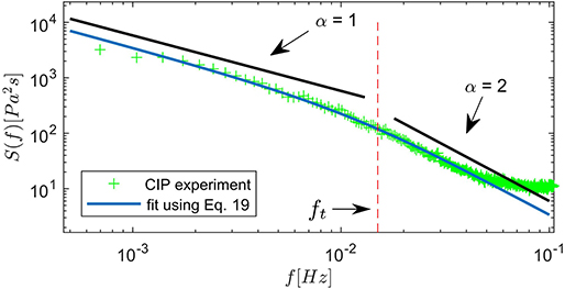
Figure 14. Comparison between theory (thin blue line) and experiments (green crosses) for the CIP PSD. The theoretical prediction is given by Equation (19), in which we have used $f_t=1.5·10^{-2}$ Hz (marked as a dashed red line) and A²r = 1.35 Pa²/s. Guide-to-eye lines with exponents corresponding to the 1/f (pink noise) and 1/f² (brown noise) regions are also shown (thick black lines). The fit indicates the correctness of the asymptotic forms presented in Equation (20) and, more importantly, that this theory correctly captures the scaling features of the experimental PSD. Adapted from Moura et al. [23] under the Creative Commons CCBY license.

Additional refinements of the model are still possible, even without losing the benefit of analytical tractability. One could, for instance, think of a model in which not only the pulses decaying rates λ, but also their amplitudes A follow a certain distribution. The calculations can be handled out in a similar manner, under the assumption that the distributions of λ and A are uncorrelated, the only difference being the fact that the constant value A² in Equation (17) would be exchanged by the expected value of this quantity. The resulting equation for a model with A being distributed according to a given probability density function ϑ(A) between two positive endpoint values A₁ and A₂, with A₂ > A₁ and having λ again following a uniform distribution is

$\begin{array}{l}{S}^{Ag}=\frac{r}{({\lambda }_2-{\lambda }_1)2\pi f}{\displaystyle {\int }_{A_1}^{A_2}}{A}^2\vartheta \left(A\right)dA\\ \left(arctan\left(\frac{{\lambda }_2}{2\pi f}\right)-arctan\left(\frac{{\lambda }_1}{2\pi f}\right)\right),& (21)\end{array}$

in which the superscripts in S^Ag denotes a general distribution in the amplitudes A, the distribution of the decaying rates λ remaining uniform. Notice that, this change will not interfere with the frequency dependency of S. Therefore, the power spectrum of a model with any distribution of amplitudes A and a uniform distribution of decaying rates λ still presents the same scaling behaviors as the one shown in Equation (18), in particular, it could also be used to explain the 1/f to 1/f² transition (pink to brown noise transition) observed in our experiments. Indeed, from Figure 7B, one would expect that the pulse amplitudes should follow some sort of distribution instead of assuming a single constant value. Nevertheless, considering that we are currently not measuring the product A²r (or its expected value in Equation 21) but merely using it as a fitting parameter in the theory, we have chosen to use the simplified version as in Equation (20) since this is sufficient to capture the relevant scaling features.

Finally, as a last step of generalization in the model, one could consider the scenario in which the condition of a uniform distribution for the decaying rates λ is also lifted. By considering a power-law distribution of the form

$\begin{array}{ll}{\upsilon }_p(\lambda )=k{\lambda }^{-\delta },& (22)\end{array}$

between the positive endpoints λ₁ and λ₂, with λ₂ > λ₁. The subscript in υ_p denotes a power-law distribution and k is a normalization constant. The case δ = 0 corresponds to the one in Equation (14). Using this distribution, together with Equations (15) and (21) we obtain the general form for the power spectrum of a model with an arbitrary distribution ϑ(A) of amplitudes and a power-law distribution υ_p(λ) of decaying times. This model is, surprisingly, still integrable (similar calculations can be found in Butz [93]). The integration of Equation (15) results in

$\begin{array}{ll}{S}_{\lambda p}^{Ag}(f)=kr{\displaystyle {\int }_{A_1}^{A_2}}{A}^2\vartheta (A)dA\stackrel{I(f)}{\overbrace{{\displaystyle {\int }_{{\lambda }_1}^{{\lambda }_2}}\frac{{\lambda }^{-\delta }}{{\lambda }^2+4{\pi }^2{f}^2}d\lambda }},& (23)\end{array}$

where,

$\begin{array}{ll}I(f)=\{\begin{array}{ll}{\frac{1}{4{\pi }^2{f}^2}\ln \frac{\lambda }{\sqrt{{\lambda }^2+4{\pi }^2{f}^2}}|}_{{\lambda }_1}^{\lambda 2}\hfill & \text{if }\delta \text{=1}\hfill \\ \frac{{\lambda }^{1-\delta }}{\left(1-\delta \right)4{\pi }^2{f}^2}\hfill & \hfill \\ {{}_2{F}_1\left(\frac{1-\delta }{2},1;1+\frac{1-\delta }{2};-\frac{{\lambda }^2}{4{\pi }^2{f}^2}\right)|}_{{\lambda }_1}^{\lambda 2}\hfill & \text{if }\delta \ne 1,\hfill \end{array}\hfill & (24)\end{array}$

and ₂F₁(a, b; c; z) is the Gauss hypergeometric function [90]. The subscript and superscript in $S_{\lambda p}^{Ag}$ denote a general distribution in the amplitudes A and a power-law distribution for the decaying rates λ. The fact that this model admits an analytical solution even for these conditions is surely worth noticing, nevertheless, the complicated form of Equations (23) and (24) does not yield much insight into the actual frequency dependency of $S_{Ag}^{\lambda p}$. Since this dependency is entirely encoded in the I(f) term in Equation (23), one can perform a linearization procedure to analyze the behavior for very small and very large frequencies, in a similar manner to what was done earlier to produce Equation (18). The resulting behavior for very small and very large frequencies is similar to what was obtained in the case of a uniform distribution of decaying rates, i.e., I(f) ∝ 1/f⁰ if 2πf ≪ λ₁ and I(f) ∝ 1/f² if 2πf ≫ λ₂. Therefore, the limiting cases exhibit the same white and brown noise profile. In the intermediate frequency range, i.e., λ₁ ≪ 2πf ≪ λ₂, one can perform the change in variables u = λ/(2πf) to rewrite I(f) as

$\begin{array}{l}I(f)=\frac{1}{{(2\pi f)}^{1+\delta }}{\displaystyle {\int }_{\frac{{\lambda }_1}{2\pi f}}^{\frac{{\lambda }_2}{2\pi f}}}\frac{u^{-\delta }}{1+u^2}du\\ \approx \frac{1}{{(2\pi f)}^{1+\delta }}{\displaystyle {\int }_0^{\infty }}\frac{u^{-\delta }}{1+u^2}du.& (25)\end{array}$

The resulting integral converges and we conclude that in the intermediate frequency range λ₁ ≪ 2πf ≪ λ₂, I(f) scales as I(f) ∝ 1/f^1+δ. By plugging this result into Equation (23), we see that $S_{\lambda p}^{Ag}(f)$ follows the same scaling, i.e.,

$\begin{array}{ll}{S}_{\lambda p}^{Ag}(f)\approx \frac{kr}{{(2\pi f)}^{1+\delta }}{\displaystyle {\int }_{A_1}^{A_2}}{A}^2\vartheta (A)dA{\displaystyle {\int }_0^{\infty }}\frac{u^{-\delta }}{1+u^2}du.& (26)\end{array}$

By changing the exponent δ characterizing the distribution of decaying rates υ_p(λ) this model can generate a whole family of 1/f^1+δ scaling regimes.

Notice that the essential assumption in the model that is necessary to account for the 1/f region is the uniform distribution of decaying rates λ. Measuring this distribution directly from the pressure signal is not viable, given that recovering the underlying exponential bursts becomes very troublesome, particularly in the region in which several bursts appear in superposition (see inset of Figure 7). In Moura et al. [23] we show evidence for the claim that λ follows a nearly uniform distribution by considering the distribution of burst's durations Θ (as defined in section 3.2).

4. Conclusions

We have performed an experimental investigation of two-phase flow phenomena in porous media, with particular focus on the question of how different boundary conditions influence the morphology of the flow and the underlying burst dynamics. We have observed that the invasion patterns are very similar for both boundary conditions, as long as the experiments are performed slowly (such as to guarantee that viscous forces are not relevant to the dynamics, which is dominated by capillary forces). Nevertheless, when it comes to dynamical features, some clear differences are observed. For example, the measured pressure signal presents pulses with a relaxation phase almost linear for the CWR boundary condition, whereas in the CIP case an exponential relaxation behavior is observed. We have analyzed the CWR pressure signal in terms of time-directed avalanches and showed how its scaling properties are in line with other works [85] in which those avalanches were investigated for systems with and without a correlated pore structure. Further on, we have shown that the differences between the CWR and CIP pressure signals are translated into their power spectral density, which, in the particular case of the CIP boundary condition, presents a 1/f scaling regime for low frequencies (pink noise), which then changes to 1/f² for intermediate frequencies (brown noise). This interesting scaling behavior is further described by a fully integrable mathematical framework in which the signal is modeled as a superposition of random exponential pulses. We have derived an expression for the PSD that was successful in describing our experiment (Equation 19) and showed how the model could be extended to a much more general class of systems, with less restricting assumptions on the distribution of pulse amplitudes and decay rates (Equations 23–26). By providing a rather general set of analytical expressions for the PSD, we hope this work will find applicability in a class of problems much wider than the specific case treated here.

Although all experiments performed employed quasi-2D samples, we believe some of our results could extend to 3D systems. In particular, the scaling features of the pressure signal power spectrum, should depend only on the intermittent dynamics of the pressure pulses, their exponential relaxation behavior and the distribution of decaying rates λ. We don't expect those properties to be a function of the dimensionality of the system, therefore, as long as the dynamics is driven in such a way that the system is in a quasi-equilibrium state, a CIP system in 3D should also present a similar 1/f to 1/f² transition in the PSD. Nevertheless, devising an experiment to perform this test in 3D is a challenging task, since the feedback mechanism used to guarantee the quasi-equilibrium state is based on the imaging of the flow and such imaging is harder to perform in 3D. One possible way to overcome this issue is to adapt the feedback mechanism to use the weight of the displaced fluid as a ruling parameter, thus lifting the need for full visualization of the flow.

Data Availability Statement

The datasets related to this study can be obtained from the corresponding author upon request.

Author Contributions

The experiments were performed and analyzed by MM, who was also responsible for writing the article. The experimental work was developed in the labs of KM, who also contributed to the definition of the research questions and the development of the experimental techniques employed. MM, KM, EF, and RT were involved in discussions that led to the theoretical analysis presented. All authors contributed actively in all stages of the work.

Funding

This work was funded by the Research Council of Norway through its Centre of Excellence funding scheme with project number 262644.

Conflict of Interest

The authors declare that the research was conducted in the absence of any commercial or financial relationships that could be construed as a potential conflict of interest.

Acknowledgments

We gratefully acknowledge the support from the University of Oslo, University of Strasbourg, the Research Council of Norway through its Centre of Excellence funding scheme with project number 262644, the CNRS-INSU ALEAS program, the LIA France-Norway D-FFRACT, and the EU Marie Curie ITN FLOWTRANS network. We would also like to thank Mihailo Jankov, James Campbell, and Kristian Olsen for many fruitful discussions. Finally, we would like to express our gratitude for the very constructive feedback obtained from the reviewers in the production of this work.

Supplementary Material

The Supplementary Material for this article can be found online at: https://www.frontiersin.org/articles/10.3389/fphy.2019.00217/full#supplementary-material

References

1. Bear J. Dynamics of Fluids in Porous Media. New York, NY: Elsevier (1972).

Google Scholar

2. Måløy KJ, Feder J, Jøssang T. Viscous fingering fractals in porous media. Phys Rev Lett. (1985) 55:2688–91.

Google Scholar

3. Måløy KJ, Furuberg L, Feder J, Jøssang T. Dynamics of slow drainage in porous media. Phys Rev Lett. (1992) 68:2161–4. doi: 10.1103/PhysRevLett.68.2161

CrossRef Full Text | Google Scholar

4. Lenormand R. Flow through porous media: limits of fractal pattern. Proc R Soc Lond A. (1989) 423:159–16.

Google Scholar

5. Lenormand R, Zarcone C. Capillary fingering: percolation and fractal dimension. Transp Porous Media. (1989) 4:599–612. doi: 10.1007/BF00223630

CrossRef Full Text | Google Scholar

6. Løvoll G, Méheust Y, Måløy KJ, Aker E, Schmittbuhl J. Competition of gravity, capillary and viscous forces during drainage in a two-dimensional porous medium, a pore scale study. Energy. (2005) 30:861–72. doi: 10.1016/j.energy.2004.03.100

CrossRef Full Text | Google Scholar

7. Or D. Scaling of capillary, gravity and viscous forces affecting flow morphology in unsaturated porous media. Adv Water Resour. (2008) 31:1129–36. doi: 10.1016/j.advwatres.2007.10.004

CrossRef Full Text | Google Scholar

8. Toussaint R, Måløy KJ, Méheust Y, Løvoll G, Jankov M, Schäfer G, et al. Two-Phase flow: structure, upscaling, and consequences for macroscopic transport properties. Vadose Zone J. (2012) 11:vzj2011.0123. doi: 10.2136/vzj2011.0123

CrossRef Full Text | Google Scholar

9. Berg S, Ott H, Klapp SA, Schwing A, Neiteler R, Brussee N, et al. Real-time 3D imaging of Haines jumps in porous media flow. Proc Natl Acad Sci USA. (2013) 110:3755–9. doi: 10.1073/pnas.1221373110

PubMed Abstract | CrossRef Full Text | Google Scholar

10. Moebius F, Or D. Pore scale dynamics underlying the motion of drainage fronts in porous media. Water Resour Res. (2014) 50:8441–57. doi: 10.1002/2014WR015916

CrossRef Full Text | Google Scholar

11. Schlüter S, Berg S, Li T, Vogel HJ, Wildenschild D. Time scales of relaxation dynamics during transient conditions in two-phase flow. Water Resour Res. (2017) 53:4709–24. doi: 10.1002/2016WR019815

CrossRef Full Text | Google Scholar

12. Stokes JP, Weitz DA, Gollub JP, Dougherty A, Robbins MO, Chaikin PM, et al. Interfacial stability of immiscible displacement in a porous medium. Phys Rev Lett. (1986) 57:1718–21. doi: 10.1103/PhysRevLett.57.1718

PubMed Abstract | CrossRef Full Text | Google Scholar

13. Sandnes B, Knudsen HA, Måløy KJ, Flekkøy EG. Labyrinth patterns in confined granular-fluid systems. Phys Rev Lett. (2007) 99:038001. doi: 10.1103/PhysRevLett.99.038001

PubMed Abstract | CrossRef Full Text | Google Scholar

14. Knudsen HA, Sandnes B, Flekkøy EG, Måløy KJ. Granular labyrinth structures in confined geometries. Phys Rev E. (2008) 77:021301 doi: 10.1103/PhysRevE.77.021301

PubMed Abstract | CrossRef Full Text | Google Scholar

15. Sandnes B, Flekkøy EG, Knudsen HA, Måløy KJ, See H. Patterns and flow in frictional fluid dynamics. Nat Commun. (2011) 2:288. doi: 10.1038/ncomms1289

PubMed Abstract | CrossRef Full Text | Google Scholar

16. Eriksen FK, Toussaint R, Måløy KJ, Flekkøy EG. Invasion patterns during two-phase flow in deformable porous media. Front Phys. (2015) 3:81. doi: 10.3389/fphy.2015.00081

CrossRef Full Text | Google Scholar

17. Dumazer G, Sandnes B, Ayaz M, Måløy KJ, Flekkøy EG. Frictional fluid dynamics and plug formation in multiphase millifluidic flow. Phys Rev Lett. (2016) 117:028002. doi: 10.1103/PhysRevLett.117.028002

PubMed Abstract | CrossRef Full Text | Google Scholar

18. Eriksen JA, Toussaint R, Måløy KJ, Flekkøy E, Galland O, Sandnes B. Pattern formation of frictional fingers in a gravitational potential. Phys Rev Fluids. (2018) 3:013801. doi: 10.1103/PhysRevFluids.3.013801

CrossRef Full Text | Google Scholar

19. Furuberg L, Måløy KJ, Feder J. Intermittent behavior in slow drainage. Phys Rev E. (1996) 53:966–77. doi: 10.1103/PhysRevE.53.966

PubMed Abstract | CrossRef Full Text | Google Scholar

20. Santucci S, Planet R, Måløy KJ, Ortín J. Avalanches of imbibition fronts: towards critical pinning. Europhys Lett. (2011) 94:46005. doi: 10.1209/0295-5075/94/46005

CrossRef Full Text | Google Scholar

21. Clotet X, Ortín J, Santucci S. Experimental study of stable imbibition displacements in a model open fracture. I. Local avalanche dynamics. Phys Rev E. (2016) 93:012149. doi: 10.1103/PhysRevE.93.012149

PubMed Abstract | CrossRef Full Text | Google Scholar

22. Eriksen FK, Toussaint R, Turquet AL, Måløy KJ, Flekkøy EG. Pneumatic fractures in confined granular media. Phys Rev E. (2017) 95:062901. doi: 10.1103/PhysRevE.95.062901

PubMed Abstract | CrossRef Full Text | Google Scholar

23. Moura M, Måløy KJ, Toussaint R. Critical behavior in porous media flow. Europhys Lett. (2017) 118:14004. doi: 10.1209/0295-5075/118/14004

CrossRef Full Text | Google Scholar

24. Moura M, Måløy KJ, Flekkøy EG, Toussaint R. Verification of a dynamic scaling for the pair correlation function during the slow drainage of a porous medium. Phys Rev Lett. (2017) 119:154503. doi: 10.1103/PhysRevLett.119.154503

PubMed Abstract | CrossRef Full Text | Google Scholar

25. Cieplak M, Robbins MO. Dynamical transition in quasistatic fluid invasion in porous media. Phys Rev Lett. (1988) 60:2042–5. doi: 10.1103/PhysRevLett.60.2042

PubMed Abstract | CrossRef Full Text | Google Scholar

26. Cieplak M, Robbins MO. Influence of contact angle on quasistatic fluid invasion of porous media. Phys Rev B. (1990) 41:11508–21.

PubMed Abstract | Google Scholar

27. Holtzman R, Segre E. Wettability stabilizes fluid invasion into porous media via nonlocal, cooperative pore filling. Phys Rev Lett. (2015) 115:164501. doi: 10.1103/PhysRevLett.115.164501

PubMed Abstract | CrossRef Full Text | Google Scholar

28. Trojer M, Szulczewski ML, Juanes R. Stabilizing fluid-fluid displacements in porous media through wettability alteration. Phys Rev Appl. (2015) 3:054008. doi: 10.1103/PhysRevApplied.3.054008

CrossRef Full Text | Google Scholar

29. Helland JO, Friis HA, Jettestuen E, Skjæveland SM. Footprints of spontaneous fluid redistribution on capillary pressure in porous rock. Geophys Res Lett. (2017) 44:4933–43. doi: 10.1002/2017GL073442

CrossRef Full Text | Google Scholar

30. Guymon G. Unsaturated Zone Hydrology. Upper Saddle River, NJ: Prentice Hall (1994). Available online at: https://books.google.no/books?id=rwpo5ReiOHUC&pg=PT3&lpg=PT3&dq=guymon+unsaturated+zone&source=bl&ots=krREK2egO4&sig=ACfU3U2rM0mLw0E1sqQPy19H5i5tuGuuqw&hl=en&sa=X&ved=2ahUKEwiNvruN9bfmAhVS_CoKHTUuAIIQ6AEwCHoECAoQAQ#v=onepage&q=guymon%20unsaturated%20zone&f=false

Google Scholar

31. Bear J. Dynamics of Fluids in Porous Media. Dover Publications (2013).

Google Scholar

32. Bear J, Verruijt A. Modeling Groundwater Flow and Pollution. Dordrecht; Boston, MA; Norwell, MA: D. Reidel Pub. Co. Sold; distributed in the U.S.A; Canada by Kluwer Academic Publishers (1987).

Google Scholar

33. Jellali S, Muntzer P, Razakarisoa O, Schäfer G. Large scale experiment on transport of trichloroethylene in a controlled aquifer. Transp Porous Media. (2001) 44:145–63. doi: 10.1023/A%3A1010652230922

CrossRef Full Text | Google Scholar

34. Nsir K, Schäfer G, di Chiara Roupert R, Razakarisoa O, Toussaint R. Laboratory experiments on DNAPL gravity fingering in water-saturated porous media. Int J Multiphase Flow. (2012) 40:83–92. doi: 10.1016/j.ijmultiphaseflow.2011.12.003

CrossRef Full Text | Google Scholar

35. Lake L. Enhanced Oil Recovery. Englewood Cliffs, NJ: Prentice Hall (1989).

Google Scholar

36. Marle C. Multiphase Flow in Porous Media. Paris; Houston, TX: Editions technip Gulf Pub. Co (1981).

Google Scholar

37. England WA, Mackenzie AS, Mann DM, Quigley TM. The movement and entrapment of petroleum fluids in the subsurface. J Geol Soc. (1987) 144:327–47.

Google Scholar

38. Tweheyo MT, Holt T, Torsæter O. An experimental study of the relationship between wettability and oil production characteristics. J Petrol Sci Eng. (1999) 24:179–88.

Google Scholar

39. Luo X, Yu J, Zhang L, Yang Y, Chen R, Chen Z, et al. Numerical modeling of secondary migration and its applications to Chang-6 Member of Yanchang Formation (Upper Triassic), Longdong area, Ordos Basin, China. Sci China Ser D Earth Sci. (2007) 50:91–102. doi: 10.1007/s11430-007-6019-9

CrossRef Full Text | Google Scholar

40. Shabani Afrapoli M, Alipour S, Torsæter O. Fundamental study of pore scale mechanisms in microbial improved oil recovery processes. Transp Porous Media. (2011) 90:949–64. doi: 10.1007/s11242-011-9825-7

CrossRef Full Text | Google Scholar

41. Yan J, Luo X, Wang W, Toussaint R, Schmittbuhl J, Vasseur G, et al. An experimental study of secondary oil migration in a three-dimensional tilted porous medium. AAPG Bull. (2012) 96:773–88. doi: 10.1306/09091110140

CrossRef Full Text | Google Scholar

42. Vasseur G, Luo X, Yan J, Loggia D, Toussaint R, Schmittbuhl J. Flow regime associated with vertical secondary migration. Mar Petrol Geol. (2013) 45:150–8. doi: 10.1016/j.marpetgeo.2013.04.020

CrossRef Full Text | Google Scholar

43. Anderson R, Zhang L, Ding Y, Blanco M, Bi X, Wilkinson DP. A critical review of two-phase flow in gas flow channels of proton exchange membrane fuel cells. J Power Sources. (2010) 195:4531–53. doi: 10.1016/j.jpowsour.2009.12.123

CrossRef Full Text | Google Scholar

44. Hwang SH, Kim C, Song H, Son S, Jang J. Designed architecture of multiscale porous TiO2 nanofibers for dye-sensitized solar cells photoanode. ACS Appl Mater Interfaces. (2012) 4:5287–92. doi: 10.1021/am301245s

PubMed Abstract | CrossRef Full Text | Google Scholar

45. Wilkinson D, Willemsen JF. Invasion percolation: a new form of percolation theory. J Phys A Math Gen. (1983) 16:3365–76.

Google Scholar

46. Furuberg L, Feder J, Aharony A, Jøssang T. Dynamics of invasion percolation. Phys Rev Lett. (1988) 61:2117–20. doi: 10.1103/PhysRevLett.61.2117

PubMed Abstract | CrossRef Full Text | Google Scholar

47. Tuller M, Or D, Dudley LM. Adsorption and capillary condensation in porous media: Liquid retention and interfacial configurations in angular pores. Water Resour Res. (1999) 35:1949–64. doi: 10.1029/1999WR900098

CrossRef Full Text | Google Scholar

48. Or D, Tuller M. Liquid retention and interfacial area in variably saturated porous media: Upscaling from single-pore to sample-scale model. Water Resour Res. (1999) 35:3591–605. doi: 10.1029/1999WR900262

CrossRef Full Text | Google Scholar

49. Méheust Y, Løvoll G, Måløy KJ, Schmittbuhl J. Interface scaling in a two-dimensional porous medium under combined viscous, gravity, and capillary effects. Phys Rev E. (2002) 66:051603. doi: 10.1103/PhysRevE.66.051603

PubMed Abstract | CrossRef Full Text | Google Scholar

50. Toussaint R, Løvoll G, Méheust Y, Måløy KJ, Schmittbuhl J. Influence of pore-scale disorder on viscous fingering during drainage. Europhys Lett. (2005) 71:583–9. doi: 10.1209/epl/i2005-10136-9

CrossRef Full Text | Google Scholar

51. Polak S, Cinar Y, Holt T, Torsæter O. An experimental investigation of the balance between capillary, viscous, and gravitational forces during CO2 injection into saline aquifers. Energy Procedia. (2011) 4:4395–02. doi: 10.1016/j.egypro.2011.02.392

CrossRef Full Text | Google Scholar

52. Moebius F, Or D. Interfacial jumps and pressure bursts during fluid displacement in interacting irregular capillaries. J Colloid Interface Sci. (2012) 377:406–15. doi: 10.1016/j.jcis.2012.03.070

PubMed Abstract | CrossRef Full Text | Google Scholar

53. Haines WB. Studies in the physical properties of soil. V. The hysteresis effect in capillary properties, and the modes of moisture distribution associated therewith. J Agric Sci. (1930) 20:97–116.

Google Scholar

54. Lenormand R, Zarcone C, Sarr A. Mechanisms of the displacement of one fluid by another in a network of capillary ducts. J Fluid Mech. (1983) 135:337–53.

Google Scholar

55. Misztal M, Hernandez Garcia A, Matin R, Müter D, Jha D, Søensen H, et al. Simulating anomalous dispersion in porous media using the unstructured lattice Boltzmann method. Front Phys. (2015) 3:50. doi: 10.3389/fphy.2015.00050

CrossRef Full Text | Google Scholar

56. Pomeau Y, Manneville P. Intermittent transition to turbulence in dissipative dynamical systems. Commun Math Phys. (1980) 74:189–97. doi: 10.1007/BF01197757

CrossRef Full Text | Google Scholar

57. Manneville P. Intermittency, self-similarity and 1/f spectrum in dissipative dynamical systems. J Phys. (1980) 41:1235–43. doi: 10.1051/jphys:0198000410110123500

CrossRef Full Text | Google Scholar

58. Hirsch JE, Huberman BA, Scalapino DJ. Theory of intermittency. Phys Rev A. (1982) 25:519–32. doi: 10.1103/PhysRevA.25.519

CrossRef Full Text | Google Scholar

59. Burlaga LF. Intermittent turbulence in the solar wind. J Geophys Res. (1991) 96:5847–51. doi: 10.1029/91JA00087

CrossRef Full Text | Google Scholar

60. Ruzmaikin AA, Feynman J, Goldstein BE, Smith EJ, Balogh A. Intermittent turbulence in solar wind from the south polar hole. J Geophys Res. (1995) 100:3395–403. doi: 10.1029/94JA02808

CrossRef Full Text | Google Scholar

61. Sneppen K, Bak P, Flyvbjerg H, Jensen MH. Evolution as a self-organized critical phenomenon. Proc Natl Acad Sci USA. (1995) 92:5209–13.

PubMed Abstract | Google Scholar

62. Gomes MAF, Souza FAO, Brito VP. Persistence and intermittency in sliding of blocks. J Phys D Appl Phys. (1998) 31:3223.

Google Scholar

63. Liu Y, Gopikrishnan P, Cizeau P, Meyer M, Peng CK, Stanley HE. Statistical properties of the volatility of price fluctuations. Phys Rev E. (1999) 60:1390–400. doi: 10.1103/PhysRevE.60.1390

PubMed Abstract | CrossRef Full Text | Google Scholar

64. Sethna JP, Dahmen KA, Myers CR. Crackling noise. Nature. (2001) 410:242–50. doi: 10.1038/35065675

PubMed Abstract | CrossRef Full Text | Google Scholar

65. Måløy KJ, Santucci S, Schmittbuhl J, Toussaint R. Local waiting time fluctuations along a randomly pinned crack front. Phys Rev Lett. (2006) 96:045501 doi: 10.1103/PhysRevLett.96.045501

PubMed Abstract | CrossRef Full Text | Google Scholar

66. Grob M, Schmittbuhl J, Toussaint R, Rivera L, Santucci S, Måløy KJ. Quake catalogs from an optical monitoring of an interfacial crack propagation. Pure Appl Geophys. (2009) 166:777–99. doi: 10.1007/s00024-004-0496-z

CrossRef Full Text | Google Scholar

67. Planet R, Santucci S, Ortín J. Avalanches and Non-gaussian fluctuations of the global velocity of imbibition fronts. Phys Rev Lett. (2009) 102:094502. doi: 10.1103/PhysRevLett.102.094502

PubMed Abstract | CrossRef Full Text | Google Scholar

68. Salazar DSP, Vasconcelos GL. Stochastic dynamical model of intermittency in fully developed turbulence. Phys Rev E. (2010) 82:047301. doi: 10.1103/PhysRevE.82.047301

PubMed Abstract | CrossRef Full Text | Google Scholar

69. Tallakstad KT, Toussaint R, Santucci S, Schmittbuhl J, Måløy KJ. Local dynamics of a randomly pinned crack front during creep and forced propagation: an experimental study. Phys Rev E. (2011) 83:046108. doi: 10.1103/PhysRevE.83.046108

PubMed Abstract | CrossRef Full Text | Google Scholar

70. Tallakstad KT, Toussaint R, Santucci S, Måløy KJ. Non-gaussian nature of fracture and the survival of fat-tail exponents. Phys Rev Lett. (2013) 110:145501. doi: 10.1103/PhysRevLett.110.145501

PubMed Abstract | CrossRef Full Text | Google Scholar

71. Stojanova M, Santucci S, Vanel L, Ramos O. High frequency monitoring reveals aftershocks in subcritical crack growth. Phys Rev Lett. (2014) 112:115502. doi: 10.1103/PhysRevLett.112.115502

PubMed Abstract | CrossRef Full Text | Google Scholar

72. Roux S, Guyon E. Temporal development of invasion percolation. J Phys A. (1989) 22:3693.

Google Scholar

73. Hele-Shaw HS. The flow of water. Nature. (1898) 58:34–6.

Google Scholar

74. Moura M, Fiorentino EA, Måløy KJ, Schäfer G, Toussaint R. Impact of sample geometry on the measurement of pressure-saturation curves: Experiments and simulations. Water Resour Res. (2015) 51:8900–26. doi: 10.1002/2015WR017196

CrossRef Full Text | Google Scholar

75. Løvoll G, Jankov M, Måløy KJ, Toussaint R, Schmittbuhl J, Schäfer G, et al. Influence of viscous fingering on dynamic saturation-pressure curves in porous media. Transp Porous Media. (2011) 86:305–24. doi: 10.1007/s11242-010-9622-8

CrossRef Full Text | Google Scholar

76. Martys N, Robbins MO, Cieplak M. Scaling relations for interface motion through disordered media: Application to two-dimensional fluid invasion. Phys Rev B. (1991) 44:12294–306. doi: 10.1103/PhysRevB.44.12294

PubMed Abstract | CrossRef Full Text | Google Scholar

77. Paczuski M, Maslov S, Bak P. Avalanche dynamics in evolution, growth, and depinning models. Phys Rev E. (1996) 53:414–43. doi: 10.1103/PhysRevE.53.414

PubMed Abstract | CrossRef Full Text | Google Scholar

78. Jankov M, Løvoll G, Knudsen HA, Måløy KJ, Planet R, Toussaint R, et al. Effects of pressure oscillations on drainage in an elastic porous medium. Transp Porous Media. (2010) 84:569–85. doi: 10.1007/s11242-009-9521-z

CrossRef Full Text | Google Scholar

79. Feder J. Fractals. New York, NY: Plenum Press (1988).

Google Scholar

80. Schroeder MR. Fractals, Chaos, Power Laws : Minutes From an Infinite Paradise. New York, NY: W.H. Freeman (1991).

Google Scholar

81. Stauffer D. Introduction to Percolation Theory. London; Bristol, PA: Taylor & Francis (1994).

Google Scholar

82. Morrow NR. Physics and thermodynamics of capillary action in porous media. Indus Eng Chem. (1970) 62:32–56. doi: 10.1021/ie50726a006

CrossRef Full Text | Google Scholar

83. Maslov S. Time directed avalanches in invasion models. Phys Rev Lett. (1995) 74:562–5. doi: 10.1103/PhysRevLett.74.562

PubMed Abstract | CrossRef Full Text | Google Scholar

84. Aker E, Måløy KJ, Hansen A, Basak S. Burst dynamics during drainage displacements in porous media: simulations and experiments. Europhys Lett. 2000 51:55–61. doi: 10.1209/epl/i2000-00331-2

CrossRef Full Text | Google Scholar

85. Biswas S, Fantinel P, Borgman O, Holtzman R, Goehring L. Drying and percolation in correlated porous media. Phys Rev Fluids. (2018) 3:124307. doi: 10.1103/PhysRevFluids.3.124307

CrossRef Full Text | Google Scholar

86. Johnson JB. The schottky effect in low frequency circuits. Phys Rev. (1925) 26:71–85.

Google Scholar

87. Ziel AVD. On the noise spectra of semi-conductor noise and of flicker effect. Physica. (1950) 16:359–72.

Google Scholar

88. Bernamont J. Fluctuations de potential aux bornes d'un conducteur metallique de faible volume parcouru par un courant. Ann Phys. (1937) 7:71–140.

Google Scholar

89. Milotti E. 1/f noise: a pedagogical review. ArXiv Physics e-prints. (2002).

Google Scholar

90. Hassani S. Mathematical Physics: A Modern Introduction to Its Foundations. New York, NY: Springer (1999).

Google Scholar

91. Welch P. The use of fast Fourier transform for the estimation of power spectra: A method based on time averaging over short, modified periodograms. IEEE Trans Audio Electroacoust. (1967) 15:70–3.

Google Scholar

92. Press W. Numerical Recipes in FORTRAN: The Art of Scientific Computing. Cambridge; New York, NY: Cambridge University Press (1992).

Google Scholar

93. Butz A. A theory of 1/f noise. J Stat Phys. (1972) 4:199–216.

Google Scholar