Risk Connectedness Heterogeneity in the Cryptocurrency Markets

1. Introduction

The cryptocurrency markets have recently seen a remarkable increase in prices, leading to some suggestion that cryptocurrencies could be considered as a new kind of financial asset. The market capitalization created by Bitcoin, the classical and most well-known cryptocurrency, grew from 10.1 to 79.7 billion during the period from Oct 2016 to Oct 2017. The price jumped from 616 to 4,800 US dollars. The high returns from the cryptocurrency markets may respond rationally to their high volatilities [2, 3]. They are characterized by a distributed payment system built on cryptographical protocols. This takes advantage of the anonymity, low cost, and fast speed of P2P transactions [4]. Cryptocurrencies are easy to generate speculative bubbles [5], which may spread contagion in return, weakening financial stability [6]. Hence, there has been a great number of papers analyzing cryptocurrencies as financial assets and aiming to identify the information transmission patterns among the cryptocurrency markets and other asset categories like equities, bonds, commodities, currencies, and so on [7–12].

A great deal of literature pays attention to relationships among cryptocurrencies and financial variables due to their roles as new asset classes [9] and important elements in the global financial market [13]. Most of them focus on Bitcoin. However, with the development of cryptocurrency markets, some newly produced cryptocurrencies like Ethereum, Ripple, Litecoin, Stellar, Monero, and Dash have gradually been cutting into the dominant share of market value taken by Bitcoin. This suggests that cryptocurrency investors are taking a breather from Bitcoin and meanwhile looking at other alternative cryptocurrencies. These new cryptocurrencies, which have taken some of the conceptual and technological advantages of Bitcoin (e.g., blockchain technology), are attracting more and more attention as well as creating a mass of opportunities for cryptocurrency investors. Actually, we have to explain that this is not a surprising event, given the fact that each alternative cryptocurrency outperformed Bitcoin in 2017, delivering astonishing returns, which ranged from 5,000% (Litecoin) to 36,000% (Ripple) compared with the 1,300% price appreciation of Bitcoin [14].

The growing interest in the new alternative cryptocurrency markets for investment purposes is accompanied by a lack of knowledge about the interaction between one leading cryptocurrency and another. In fact, the rapid development of cryptocurrency markets results in some relative heterogeneity among mainstream cryptocurrencies. It is helpful to extend the limited literature on connectedness among cryptocurrency markets for use by cryptocurrency investors in devising investment and trading strategies that may involve introducing cryptocurrencies into the portfolio. On the other hand, it is also helpful to construct connectedness networks for use by policy-makers in formulating policies aimed at preserving financial stability. Investors and risk managers can benefit from establishing a connectedness network across many asset classes to generate their investment and hedging decisions. Generally, building connectedness networks is hardly new in conventional assets. Prior works have uncovered connected network structures among or within different assets/markets, including equities [15, 16], bonds [17, 18], currencies [19, 20], commodities [21, 22], and interest rates [18]. However, few works have constructed networks of connectedness in the cryptocurrency market, which is becoming an appealing investment ground for investors. Wei [23] examined the liquidity for 456 kinds of cryptocurrencies. He showed that return predictability weakens in cryptocurrencies with high market liquidity and claimed that liquidity has a significant impact on market efficiency and return predictability for new cryptocurrencies. Yi et al. [24] focused on both static and dynamic volatility connectedness among eight leading cryptocurrencies, revealing their cyclic volatility connectedness, with an evident rising trend at the end of 2016. They linked 52 cryptocurrencies by constructing a volatility connectedness network making use of a variance decomposition framework and found that the 52 cryptocurrencies are interconnected tightly. The so-called “mega-cap” cryptocurrencies are more likely to spread volatility shocks to others. Connectedness among leading cryptocurrencies can also be investigated via return and volatility spillovers, as in Ji et al. [14], where the results achieved implied that the return of each cryptocurrency and its volatility connectedness with others did not necessarily depend heavily on its market size. Some authors have taken the perspective of evolutionary dynamics; for example, ElBahrawy et al. [25] took this approach to analyze the behavior of 1,469 cryptocurrencies and revealed some statistical properties for cryptocurrency markets.

Motivated by the current works on connectedness among the cryptocurrency markets, in this paper, we focus on risk connectedness for the sake of portfolio diversification and risk management. Risk connectedness and spillover have been widely treated, for example, connectedness among stock markets [26, 27], credit markets [28], financial institutions [29], and sovereigns [30, 31] and connectedness between stock and oil markets [32, 33], stock prices and exchange rates [34], energy and carbon markets [35], and so forth. Understanding the risk connectedness among cryptocurrency markets provides valuable information regarding investment and hedging decisions. Moreover, it also provides potential information for systematic risk in the whole cryptocurrency system, according to which the regulators can generate strategies to control risk contagion. The current paper differs from the existing literature in several ways. We use the daily data of seven leading cryptocurrencies, Bitcoin, Ethereum, Ripple, Litecoin, Stellar, Monero, and Dash, to compute their risk levels and investigate the risk connectedness among cryptocurrency markets by providing risk spillovers among these leading cryptocurrencies, accounting for more than 75% of the cryptocurrency market value. The most notable contribution of our work is heterogeneity analysis of the risk connectedness of cryptocurrencies. Two heterogeneities are considered in this paper. The first heterogeneity is the asymmetric risk spillovers at times of upward risk tendency and downward risk tendency in the cryptocurrency markets. The connectedness asymmetry under different risk tendencies is mainly determined by investor expectation. The second heterogeneity is captured by the differences in risk spillovers among the cryptocurrencies at different timescales, namely, in the short term (0–4 days), medium term (4–30 days), and long term (30–300 days). The heterogeneity of risk spillovers at different timescales mainly originates from the persistence of investor attention. Our findings are highly informative for market participants, who can adjust their hedging strategies according to different market tendencies or time horizons.

The paper is organized as follows. Section 2 details the risk measurements for the selected cryptocurrencies. Section 3 shows the static risk connectedness among the cryptocurrency markets. The heterogeneity of risk spillovers under upward risk tendency and downward risk tendency is analyzed. Section 4 explores the risk connectedness at different timescales, which shows the heterogeneity of risk spillovers among the cryptocurrencies in the short term, medium term, and long term. Section 5 concludes with some policy implications.

2. Risk Measurement for the Cryptocurrencies

It is well-known that the cryptocurrency returns are extremely volatile, with clustering phenomena. Bollerslev [36] used GARCH models to capture these characteristics well. GARCH models have been widely popular as tools for measuring market risk by the VaR method due to their relative simplicity and various extensions. Unfortunately, their limitations, especially the unrealistic parametric assumptions, such as normality or i.i.d returns, which does not fit the case of cryptocurrencies, are also evident. To overcome these problems, in this paper, we apply the semi-parametric Conditional Autoregressive Value at Risk (CAViaR) method developed by Engle and Manganelli [37] to estimate VaR models for cryptocurrencies, avoiding any extreme assumption invoked by the existing methodologies. Unlike GARCH and GAS, which model the whole distribution, CAViaR directly models the quantile of the return distribution, extending the standard quantile regression approach introduced by Koenker and Basset [38]. The CAViaR model uses an autoregressive formulation straight to the quantile.

2.1. CAViaR Model

In short, the CAViaR method is particular in estimating VaRs directly through an autoregressive specification for quantiles rather than the usual approach of inverting a conditional distribution of returns in a purely parametric framework [39]. This autoregressive dynamics for the quantile over time, as well as some unknown parameters, is then determined by the regression quantile framework [38]. Besides, the autoregressive nature of CAViaR directly captures some stylized facts in the distribution tails, like autocorrelation in daily returns arising from market microstructure biases and partial price adjustment [40], volatility clustering [36], and time-varying skewness and kurtosis [41].

In this paper, following Engle and Manganelli [37], we consider a cryptocurrency return vector ${\left\{y_t\right\}}_{t=1}^T$. Let θ be the probability associative to VaR, x_t a observable variable vector, and β_θ a unknown parameter vector. Let f_t(β) ≡ f(x_t−1, β_θ) be the θ-quantile of the cryptocurrency return distribution at time t, formed at time t − 1. Then a general CAViaR model is specified as follows:

$\begin{array}{ll}{f}_t(\beta )={\gamma }_0+{\displaystyle \sum _{i=1}^q}{\gamma }_i{f}_{t-i}(\beta )+{\displaystyle \sum _{i=1}^p}{\alpha }_{i}l(x_{t-i},\phi ),& (1)\end{array}$

where β′ = (α′, γ′, φ′) and l is the function of a finite value depending on lagged values of observable variables. Engle and Manganelli [37] introduced an autoregressive term γ_if_t−i(β), i = 1, 2, ⋯ , q, allowing a smooth transition quantile. In addition, they introduced the term l(x_t−i, φ) in order to permit a relationship between the θ-quantile f_t(β) and the observable variables. On the basis of general CAViaR formulation, Engle and Manganelli [37] developed four alternative specifications for the function l:

$\begin{array}{l}Adaptative:f_t(\beta )=f_{t-1}(\beta )+\beta ((1\\ +\text{exp}(G(y_{t-1}-f_{t-1}(\beta )))){}^{-1}-\theta ),& (2)\end{array}$

$\begin{array}{ll}SymmetricAbsoluteValue:f_t(\beta )={\beta }_1+{\beta }_2{f}_{t-1}(\beta )+{\beta }_3\left|y_{t-1}\right|,& (3)\end{array}$

$\begin{array}{l}AsymmetricSlope:f_t(\beta )={\beta }_1+{\beta }_2{f}_{t-1}(\beta )+{\beta }_3{(y_{t-1})}^{+}\\ +{\beta }_4{(y_{t-1})}^{-},& (4)\end{array}$

$\begin{array}{ll}IndirectGARCH(1,1):f_t(\beta )={({\beta }_1+{\beta }_2{f}_{t-1}^2(\beta )+{\beta }_3{y}_{t-1}^3)}^{1/2}.& (5)\end{array}$

In the first specification, G is a positively finite value satisfying that the last term converges to β₁(I(y_t−1 ≤ f_t−1(β₁) − θ)) as G → ∞, where I(·) is an indicator function. As explained by Engle and Manganelli [37], the Adaptative specification allows that whenever one exceeds one's VaR, one should directly increase it. Otherwise, one should decrease it very slightly. The second and fourth specifications both respond symmetrically to past returns with mean reverting, as the coefficient of the lagged VaR is unconstrained to equal to one. The third model is also mean reverting but with less restrictions in the sense that it permits asymmetric response to both positive and negative past returns. The asymmetric CAViaR specification has become the most popular one for practitioners due to its consideration of the skewness and kurtosis properties of financial series [29, 39, 42]. In this paper, asymmetric CAViaR is also employed for measurement of the risk of cryptocurrency returns, which is verified through test statistics (see also [43] for a cryptocurrency risk measurement study).

2.2. Data and Sample Analysis

We collected daily price data on seven cryptocurrencies, Bitcoin, Ethereum, Ripple, Litecoin, Stellar, Monero, and Dash, so as to obtain sufficient price data for the 10 largest cryptocurrencies by market capitalization listed on the website https://coinmarketcap.com. Indeed, they cover almost a two-and-a-half-year period, allowing us to make the most of our empirical results and analysis. The sample interval ranges from August 7, 2015, to February 15, 2020 (1,654 daily observations) for this paper. Each selected cryptocurrency possesses a market value exceeding 5 billion USD. The total market value of these seven cryptocurrencies represents 79.5% of the entire cryptocurrency market. The empirical study is built on daily return, calculated by the difference in the log of price.

Figure 1 shows the risk level tendencies of the seven cryptocurrencies. On the whole, the cryptocurrencies show similar risk tendencies. In particular, volatility clusterings happen during the period from the beginning of 2017 to the end of 2018, since the cryptocurrencies received substantial price appreciations during this period. We can also identify some mild peculiarities of Dash and Monero. With regard to Dash, volatility clustering was common in the whole sample period, whereas for Monero, it reached its peak earlier, in the middle of August 2016, than others, whose peaks arose during the period from the beginning of 2017 to the end of 2018. Besides, they both have wider volatility ranges.

FIGURE 1

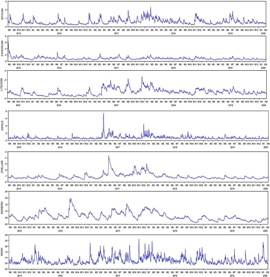
Figure 1. Risk level tendencies of the selected cryptocurrencies.

The summary statistics for the risks of cryptocurrencies, including risks under upward and downward tendencies, are given in Table 1. In Panel A, the highest mean of risk is for Stellar, followed by Ethereum and Monero together. Ripple and Stellar have the highest standard deviation, followed by Ethereum. Interestingly, as the most popular cryptocurrency in the market, Bitcoin shows the lowest mean risk and a relatively low standard deviation, only higher than Monero. In fact, these are not surprising observations. In 2017, each of the other six cryptocurrencies under study increased in value by at least 5,000%, while Bitcoin increased by 1,300%. Excess levels of kurtosis arise in all cryptocurrencies, especially Ripple. All cryptocurrencies show positive skewness. When risks increased (Panel B), Dash has the highest mean risk level and the second-highest standard deviation. Meanwhile, Ripple has the highest standard deviation and the second-highest mean risk. High levels of kurtosis and positive skewness arise in all cryptocurrencies. Litecoin occupies the highest levels in terms of both kurtosis and skewness. Moving to the statistics of decreased risks (Panel C), Stellar has the highest mean risk and standard deviation. Excess levels of kurtosis and positive skewness arise in all cryptocurrencies, where Ethereum and Ripple are dominant in both these two statistics.

TABLE 1

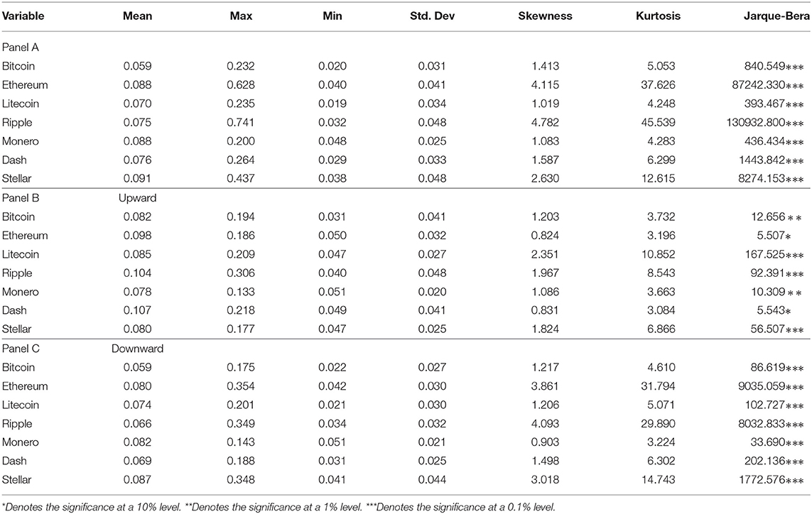
Table 1. Summary statistics for cryptocurrency risks.

The risk correlation matrices for the selected seven cryptocurrencies are shown in Table 2. Overall, weak to moderately positive correlations happen among the risk levels of the selected cryptocurrencies. In particular, the highest correlation coefficient is for the pair Bitcoin and Litecoin, given as 0.68, whereas the pair Ethereum and Stellar permits the lowest correlation coefficient given as 0.07. Focusing on the risk correlations at times of upward and downward tendencies, the correlations under an upward tendency are generally stronger than those under a downward tendency. Under an upward risk tendency, the pair Bitcoin and Ethereum has the highest correlation coefficient, 0.87, followed by the pair Ethereum and Dash, 0.79, whereas the lowest correlations are for the pairs Bitcoin and Stellar and Ethereum and Stellar, with coefficients 0.25 and 0.26, respectively. The pairs Bitcoin and Monero and Ethereum and Monero are uncorrelated under an upward risk tendency. Under a downward risk tendency, Bitcoin and Litecoin are the most positively correlated, with a coefficient of 0.70, followed by the pair Bitcoin and Dash, for which it is 0.67, while Ethereum and Stellar are uncorrelated. Overall, the correlation between Bitcoin and Litecoin is unsurprisingly much stronger than for the other pairs in the results of all three tests.

TABLE 2

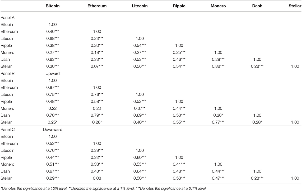
Table 2. Correlations among the cryptocurrencies.

3. Static Risk Connectedness in the Cryptocurrency Markets

We follow [1] for the methodological framework for constructing connectedness measures. In this paper, static risk connectedness networks under upward and downward tendencies, as well as static and dynamic risk connectedness at different timescales, are built.

3.1. Static Risk Connectedness Measurement

Suppose a stationary covariance seven-variable VAR(p) given as

$\begin{array}{ll}{R}_t={\displaystyle \sum _{i=1}^p}{\Phi }_i{R}_{t-i}+{\epsilon }_t,& (6)\end{array}$

where R_t is the 7 × 1 cryptocurrency risk vector, Φ_t are 7 × 7 autoregressive coefficient matrices, and ε_t is the error term vector assumed to be serially uncorrelated. If the VAR model above is a stationary covariance, then one can write a moving-average representation as

$\begin{array}{ll}{R}_t={\displaystyle \sum _{j=0}^{\infty }}{A}_j{\epsilon }_{t-j},& (7)\end{array}$

where the 7 × 7 coefficient matrix A_j obeys a recursion of the form

$\begin{array}{ll}{A}_j={\Phi }_1{A}_{j-1}+{\Phi }_2{A}_{j-2}+\cdots +{\Phi }_p{A}_{j-p},& (8)\end{array}$

where A₀ is the n × n identity matrix and A_j = 0 for j < 0. One can measure pairwise connectedness, directional connectedness, and total connectedness on the basis of a generalized forecast-error variance decomposition (FEVD) approach by using the moving-average framework. The advantage of FEVD is that it eliminates any disturbance induced in the results by the variable ordering.

Denote the H-step-ahead generalized forecast-error variance decomposition [14] by

$\begin{array}{ll}{\theta }_{ij}(H)=\frac{{\sigma }_{jj}^{-1}{\displaystyle {\sum }_{h=0}^{H-1}}{(e_i^{\prime }{A}_h\Sigma e_j)}^2}{{\displaystyle {\sum }_{h=0}^{H-1}}(e_i^{\prime }{A}_h\Sigma A_h^{\prime }{e}_i)},& (9)\end{array}$

where θ_ij(H) is the variance contribution of variable j to variable i, σ_jj is the standard deviation of the error term in the j'th equation, and Σ is the variance matrix of the error vector ε. e_i is a selection vector with a value of 1 for the i'th element. Otherwise, take it as 0. The spillover index yields an n × n matrix θ(H) = [θ_ij(H)], where each entry gives the contribution of variable j to the forecast-error variance of variable i. Own-variable and cross-variable contributions are involved in the main diagonal and off-diagonal elements, respectively, of the θ(H) matrix. Each entry in the θ(H) matrix is normalized by the row sum

$\begin{array}{ll}{\tilde{\theta }}_{ij}(H)=\frac{{\theta }_{ij}(H)}{{\displaystyle {\sum }_{j=1}^N}{\theta }_{ij}(H)},& (10)\end{array}$

to ensure that the row sum is equal to 1. There are several spillovers, such as total spillovers, directional spillovers, net spillovers, and net pairwise spillovers [14, 24, 44, 45]. In this paper, we construct the net pairwise spillovers to investigate the information spillovers among the whole cryptocurrency market system.

With respect to the net pairwise connectedness, according to the definition of FEVD, in general, ${\tilde{\theta }}_{ij}\ne {\tilde{\theta }}_{ji}$. Consequently, the difference between ${\tilde{\theta }}_{ij}$ and ${\tilde{\theta }}_{ji}$, ${\tilde{\theta }}_{ij}-{\tilde{\theta }}_{ji}$, can be used to measure the net pairwise connectedness as well as the net spillover effect from variable j to variable i. A directional connectedness network can then be built on the basis of net pairwise connectedness. Each market is regarded as a node in the network. The condition in which a directional edge from i to j exists in the network is ${\tilde{\theta }}_{ij}-{\tilde{\theta }}_{ji}>0$.

3.2. Static Risk Connectedness Over the Full Sample

Table 3 presents the matrix depicting net pairwise risk spillovers among the cryptocurrency markets, that is, net spillovers between two cryptocurrencies, where positive (negative) values mean that the cryptocurrencies in question are net receivers (transmitters) of spillover effects. Accordingly, we claim that the risk spillover is highly correlative with the capitalization of the cryptocurrency market. Mostly, risk spills over from cryptocurrencies with small capitalizations to those with large capitalizations. In particular, Bitcoin transmits little risk to Ethereum and Ripple, where the spillover indexes are given as 0.047 and 0.035%, respectively, whereas it receives more risk from Stellar, Monero, and Dash, where the spillover indexes are 1.316, 2.520, and 0.870%, respectively. Similar results are seen with regard to Ethereum, which mainly receives risks from other cryptocurrencies with small capitalizations (spillover indexes from three cryptocurrencies, Stellar, Monero, and Dash, to Ethereum are 0.462, 4.665, and 1.746%, respectively, but those from Ethereum to Ripple and Litecoin are only 0.001 and 0.034%, respectively). A similar analysis holds for Ripple and Litecoin.

TABLE 3

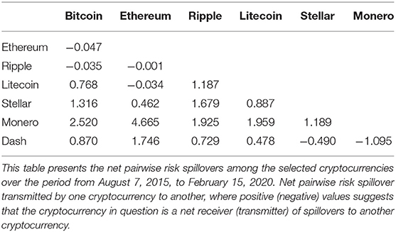
Table 3. Net pairwise risk spillover among the cryptocurrencies.

Although the empirical results we get do not agree with the return spillover directions in the existing literature, we believe that there is some relation between the risk spillover and return spillover in the cryptocurrency markets. Cryptocurrencies with large capitalization dominate the market efficiency and price fluctuation, leading the market development tendency. The rapid growth of cryptocurrencies into new classes of financial assets creates a major challenge for traditional financial markets and even impacts the whole financial market. In general, cryptocurrency investors focus on those cryptocurrencies with large capitalizations. They may take these cryptocurrencies as references when making investment strategies in the cryptocurrency markets. This results in return spillovers from cryptocurrencies with large capitalization to those with small capitalization. The return spillovers will cause violent fluctuations in cryptocurrency prices with small capitalization and then vary their return risks. The investors who intend to invest in cryptocurrencies with small capitalization still rely on the price tendencies of cryptocurrencies with large capitalization. Thus, investor attention influences the return risks of cryptocurrency markets with large capitalization, and the return risks spill over from markets with small capitalization to those with large capitalization. Indeed, this also reflects the dominant roles of cryptocurrencies with large capitalization in the whole cryptocurrency market.

3.3. Static Risk Connectedness in Upward and Downward Tendencies

Risk spillovers among the cryptocurrency markets under downward risk tendency are more remarkable than spillovers under upward risk tendency. Spillover indexes under downward risk tendency are mostly higher than those under upward risk tendency. In particular, the spillover index between Bitcoin and Ripple is shown to be −0.920% under downward risk tendency, whereas it is −0.513% under upward risk tendency. Besides, Bitcoin transmits the risks to Stellar and Dash, where the spillover indexes under downward tendency are 2.607 and 2.231%, respectively, whereas they are given correspondingly as 1.824 and 0.689% under upward tendency. Similar results are seen in Ripple and Litecoin. In fact, the asymmetrical spillover under different risk tendencies is due to the difference in the regulatory mechanism in cryptocurrency markets. Under an upward risk tendency, the cryptocurrencies not only reduce their own risks but also withstand spillovers from others more effectively. The investors generate investment strategies more prudently when the market risks are increasing. More concentrated attention on their target cryptocurrency markets results in weak spillovers among the cryptocurrencies in periods of upward risk tendency. On the contrary, markets with decreasing risks attract a large number of investors, whose confidences enhance significantly. This is again due to the regulatory mechanism of the markets themselves. The investors still pay attention to cryptocurrencies with large capitalization like Bitcoin and Ethereum, considering their dominant roles when they are generating their investment strategies. The investor attention expedites communications among the markets and impacts the risk connectedness. In summary, the cryptocurrencies spill more risks to others at times of downward risk tendency than when there is upward risk tendency. In addition, this asymmetric effect is prominent in cryptocurrencies with large capitalization.

Attention should be paid to the different spillover directions between Monero and other cryptocurrencies under upward and downward risk tendencies. One can see from Table 4 that among the twenty-one pairwise spillovers, six pairwise spillovers change their spillover directions in different risk tendencies, and four of them involve Monero. According to the signs of net pairwise spillovers, Monero mainly accepts spillovers from cryptocurrencies with large capitalization under upward risk tendency, whereas it transmits risk to these cryptocurrencies under downward risk tendency. This result agrees well with what is shown in Figure 1. In Figure 1, one can see that the risk tendency of Monero differs from those of other cryptocurrencies before the steep rise in prices of cryptocurrency markets at the beginning of 2017. Monero reached its risk peak while the other cryptocurrencies stayed in their risk troughs. However, this phenomenon disappeared after 2017. This interesting result is due to the trading volumes of cryptocurrencies. The trading volume of Monero was different from those of the others before 2017. For instance, from August 2016 to October 2016, the trading volume of Monero fluctuated strongly, whereas the others were weakly fluctuating. After 2017, the trading volume of Monero comoved with other cryptocurrencies but with a higher amplitude of fluctuation. We can capture that the differences in trading volumes between Monero and other cryptocurrencies mostly happened under downward risk tendency. The increase in cryptocurrency trading volumes drove Monero to transmit its risk to other cryptocurrencies. Thus, Monero spilled over risk, as a transmitter in the market, under a downward risk tendency. So we have to acknowledge the specific role played by Monero in the whole cryptocurrency market.

TABLE 4

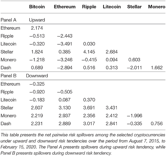
Table 4. Net pairwise risk spillover under upward and downward risk tendencies.

4. Time-Frequency Connectedness of Cryptocurrency Risks

In fact, the analysis in section 3 implies that risk connectedness among the cryptocurrency markets might show heterogeneities at different timescales, which will be verified in this section. In this section, we explore the net pairwise spillovers among the selected cryptocurrencies at different timescales, namely in the short term (<4 days), medium term (more than 4 days but <30 days), and long term (more than 30 days but <300 days). The methodology for time-frequency connectedness measurement refers to [46].

4.1. Time-Frequency Connectedness Measurements

In this paper, the spectral representation framework of generalized forecast error variance decomposition (GFEVD) is applied to the frequency decomposition. Define the generalized causation spectrum over frequency ω ∈ (−π, π) by

$\begin{array}{ll}(f(\omega )){}_{k,j}=\frac{{\Sigma }_{j,j}^{-1}|{(R(e^{-i\omega })\Sigma )}_{k,j}{|}^2}{(R(e^{-i\omega })\Sigma R^{\prime }(e^{i\omega })){}_{k,k}},& (11)\end{array}$

where $R(e^{-i\omega })=\sum _h{e}^{-i\omega h}{R}_h$, h = 1, 2, ⋯ , H, is the Fourier transform of R, with $i=\sqrt{-1}$. As noted by [46], the forecast horizon H makes no difference, since the GFEVD here is unconditional. To obtain the generalized variance decompositions on frequency band d, d ∈ (a, b), a, b ∈ (−π, π), we weight (f(ω))_{k, j} by the frequency shares of the jth volatility variance. Thus, the weighting function can be defined as

$\begin{array}{ll}{\Gamma }_k(\omega )=\frac{2(R(e^{-i\omega })\Sigma R^{\prime }(e^{i\omega })){}_{k,k}}{{\displaystyle {\int }_{-\pi }^{\pi }}(R(e^{-i\lambda })\Sigma R^{\prime }(e^{i\lambda })){}_{k,k}d\lambda }.& (12)\end{array}$

The generalized variance decompositions on frequency band d are denoted by

$\begin{array}{ll}{({\Theta }_d)}_{k,j}=\frac{1}{2}{\displaystyle {\int }_d^{\infty }}{\Gamma }_k(\omega )(f(\omega )){}_{k,j}d\omega .& (13)\end{array}$

With the spectral representation of the generalized variance decompositions, we can easily calculate the scaled generalized variance decompositions as

$\begin{array}{ll}{({\tilde{\Theta }}_d)}_{k,j}=\frac{{({\Theta }_d)}_{k,j}}{{\displaystyle {\sum }_j}{({\Theta }_{\infty })}_{k,j}},{({\Theta }_{\infty })}_{k,j}=\frac{1}{2}{\displaystyle {\int }_{-\pi }^{\pi }}{\Gamma }_k(\omega )(f(\omega )){}_{k,j}d\omega .& (14)\end{array}$

Then, the net pairwise spillovers in different frequencies are given as

$\begin{array}{ll}{S}_{k,j}=({({\tilde{\Theta }}_d)}_{k,j}-{({\tilde{\Theta }}_d)}_{j,k})·100.& (15)\end{array}$

4.2. Static Risk Connectedness at Different Timescales

Table 5 shows the static net pairwise risk spillovers among the cryptocurrency markets at short-, medium-, and long-term frequencies. It is evident that spillovers happen at medium- and long-term frequencies. Spillovers between any two cryptocurrencies are almost zero in the short term. They show signs of recovery until 4 days later. This is due to the investor attitude on the cryptocurrency markets and information exchange among them. The risk spillovers among the cryptocurrency markets result from the return spillovers and information exchange among them. As analyzed in section 3, cryptocurrencies with large capitalization play key roles in the overall market. Investment strategies are generated according to the price fluctuations of cryptocurrencies with large capitalization. Thus, investments in cryptocurrencies with small capitalization rely on the price fluctuations of cryptocurrencies with large capitalization, and so the information exchange among the cryptocurrency markets leads to risk spillovers among them. Moreover, the spillovers are not immediate but are delayed, which results from the investor attitudes and asymmetry of information. Although the investment decisions rely on the prices of cryptocurrencies with large capitalization, as emerging financial assets, cryptocurrencies are easily influenced by major events such that they show strong uncertainty. Thus, the investors first off look at the markets. On the other hand, information in the cryptocurrency markets shows asymmetry between investors and speculators, which also results in a delay in risk spillovers among the cryptocurrency markets.

TABLE 5

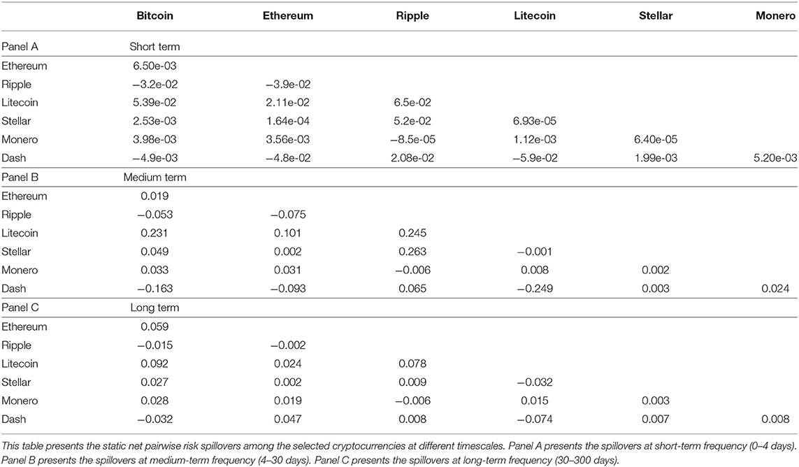
Table 5. Static net pairwise risk spillovers at different timescales.

Furthermore, comparing the net pairwise spillovers among the selected cryptocurrencies in the medium and long term in Table 5, one can catch that risk spillovers at medium-term frequency are mostly stronger than those at long-term frequency, while the spillover directions remain almost the same. In particular, only five pairwise spillover indexes at long-term frequency are larger than their corresponding indexes at medium-term frequency. Meanwhile, there is only one pairwise spillover index that changes its sign (Ethereum and Dash). The results imply that risk spillovers among the cryptocurrencies followed an upturned “U” with respect to time frequency. One may question the origin for such a phenomenon, and our reply is that it is due to dynamic investor attention on the markets. When news involving a cryptocurrency market issue or a major event enters circulation, most investors just monitor the markets without making investments, which results in slight risk spillovers among the cryptocurrencies. With sensationalization from speculators or market properties, such as trading volumes and prices varying distinctly, the investors pay their maximum attention to the markets. Considering the dominant roles of cryptocurrencies with large capitalization in the whole market, risk spillovers among the cryptocurrency markets also attain their peaks. As the market gradually acclimatizes itself to the changing information or shocks on prices caused by major events, the market efficiency of an individual cryptocurrency may increase, which reduces the risk spillovers to others. However, the increasing market efficiency of an individual cryptocurrency cannot result in a change of status in the whole market for the individual cryptocurrency. Thus, at different timescales, the risk spillover directions remain the same. Summing up, risk spillovers among the cryptocurrencies are the most remarkable in the medium term, rather than in the short term or long term. Moreover, these spillovers show persistence.

4.3. Dynamic Risk Connectedness at Different Timescales

Table 6 presents the statistics for dynamic risk connectedness among the cryptocurrency markets at medium- and long-term frequencies. The risk spillover means and ranges among the cryptocurrencies are remarkably discrepant at different timescales. In addition, several spillover directions change. The mean spillover at long-term frequency is larger than that at medium-term frequency, whereas the spillover range at medium-term frequency is wider than that at long-term frequency. In Table 6, there are sixteen pairwise spillovers whose spillover indexes at long-term frequency are larger than at medium-term frequency. Since the mean depends heavily on the length of the sample interval, we catch the dynamic characteristics of risk spillovers among the cryptocurrencies through spillover range and standard deviation. The spillover range at long-term frequency is remarkably lower than that at medium-term frequency. Similar to the analysis in subsection 4.2, this results from the collection of risk spillovers among the cryptocurrencies at medium-term frequency. The delays of price transmissions among the cryptocurrencies result in the collection of risk spillovers at medium-term frequency. Meanwhile, attentional heterogeneity in different market participants leads to wide-ranging fluctuation in risk spillover levels among the cryptocurrencies. In particular, speculators and arbitragers may get more returns due to the convenience and timeliness with which they get market information. Thus, these market participants may magnify the risk spillovers among the markets. On the other hand, speculators and arbitragers pursue medium-term profits in general, while investors prefer long-term programs. This also suggests the amplification of risk spillovers at medium-term frequency.

TABLE 6

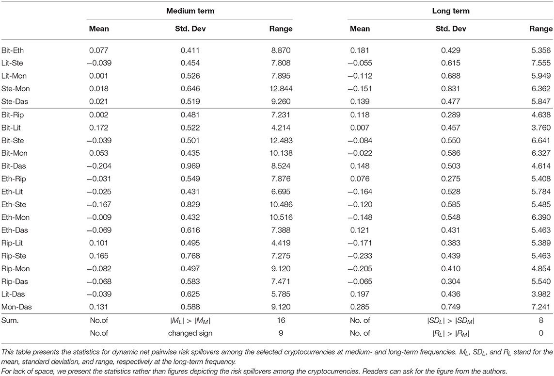
Table 6. Statistics for dynamic risk connectedness at medium- and long-term frequencies.

Referring to subsection 4.2, we divide the net pairwise spillovers into two groups. In group one, the risk spillovers at long-term frequency are stronger than those at medium-term frequency, while group two holds the inverse case. One can see from Table 6 that the risk spillover between two cryptocurrencies whose spillover at long-term frequency is stronger than that at medium-term frequency shows a strong fluctuation at long-term frequency. However, the risk spillover fluctuation at long-term frequency between two cryptocurrencies whose spillover at long-term frequency is weaker than that at medium-term frequency is remarkably weaker than that at medium-term frequency. This is due to the persistence of risk spillovers among the cryptocurrencies. In terms of Bitcoin and Ethereum, the investors will pay continuous attention to these two cryptocurrencies when they are generating investment decisions, on account of their high similarity. This leads to a longer persistence of risk spillover between Bitcoin and Ethereum, which results in the risk spillover fluctuation at long-term frequency being stronger than that at medium-term frequency. In terms of those cryptocurrencies with weak similarity, the dominant roles of cryptocurrencies with large capitalization result in stronger risk spillover fluctuations in the medium term. Summing up, we declare the heterogeneity in dynamic characteristics of risk spillovers among the cryptocurrencies at different timescales.

5. Conclusions and Policy Implications

In this paper, we study risk connectedness among the cryptocurrency markets through net pairwise risk spillover measurement. We select seven leading cryptocurrencies, Bitcoin, Ethereum, Ripple, Litecoin, Stellar, Monero, and Dash, whose capitalizations are among the top 20 in the cryptocurrency market. The data sample interval ranges from August 7, 2015, to February 15, 2020. The methodology measuring the risk spillover used in this paper is the DY index. We first explore the net pairwise risk spillovers among the selected cryptocurrencies over the whole sample. We then discuss the asymmetric spillovers at times of upward and downward risk tendency. Finally, we identify risk spillover heterogeneity at different timescales through the decomposed DY index on the basis of time frequency. The conclusion of this paper is summarized as follows.

First, the risk spillover directions are highly correlative with the capitalizations of cryptocurrencies. The risks spill over from the cryptocurrencies with small capitalization to those with large capitalization. For instance, the spillover indexes from Bitcoin to Ethereum and Ripple are 0.047 and 0.035%, respectively, while Bitcoin accepts risks from Stellar, Monero, and Dash, with spillover indexes of 1.316, 2.520, and 0.870%, respectively. Similar results also hold for Ethereum, which accepts risks from Stellar, Monero, and Dash, measured by the spillover indexes as 0.462, 4.665, and 1.746%, respectively.

Second, the risk spillovers among the cryptocurrencies under a downward risk tendency are stronger than those under an upward risk tendency. A difference in spillover direction under upward and downward risk tendencies exists in the Monero market. In particular, the risk spillover index between Bitcoin and Ripple is −0.513% under upward risk tendency while it is −0.920% under downward risk tendency. Similarly, the risk spillover indexes from Bitcoin to Stellar and Dash are 1.824 and 0.689%, respectively, under upward risk tendency, while they are 2.607 and 2.231% under downward risk tendency. Monero accepts risk transmissions from the other cryptocurrencies with large capitalization under risk upward tendency, while it transmits the risks to those cryptocurrencies in downward risk tendency. The risk spillovers in other pairs of cryptocurrencies mostly maintain the same directions under upward and downward risk tendencies.

Third, the mean and range of risk spillover at different timescales show heterogeneity. The static risk spillovers mainly happen at medium- and long-term frequencies. The risk spillovers at medium-term frequency are mostly stronger than those at long-term frequency, while the spillover directions mostly remain the same. Focusing on the dynamic characteristics of risk spillovers among the cryptocurrencies, the means of risk spillover at long-term frequency are relatively larger than those at medium-term frequency, while the ranges of risk spillovers at medium-term frequency are distinctly larger than those at long-term frequency. In addition, the risk spillover fluctuations at long-term frequency are stronger than those at medium-term frequency if the corresponding risk spillover levels maintain the same comparison at long-term and short-term frequencies. However, for cryptocurrencies whose risk spillover levels at long-term frequency are lower than at medium-term frequency, the risk spillover fluctuations at long-term frequency are distinctly weaker than those at medium-term frequency.

The empirical results have some policy implications for regulators. Regulators should establish a monitoring and warning system for risk. The risk spillovers among the cryptocurrencies show heterogeneity under different risk tendencies, whereas the spillover directions almost remain the same. Thus, a risk monitoring and warning system would be able to identify market behavior well and transmit valuable market information. In addition, some regulatory policies should aim at risk spillovers within 4–30 days. The large risk spillover fluctuations and ranges among the cryptocurrencies in the medium term pose new challenges for market supervision. Thus, the regulators should generate policies, such as determining a trading threshold, to control the risk spillovers among the cryptocurrencies, improving the market efficiency in the medium term. For the investors, the delayed effect of risk spillovers among the cryptocurrencies should be paid attention to when generating investment strategies. Major events may shock the cryptocurrency markets strongly. Study of the delayed effects of the shocks helps investors generate investment strategies unifying their own situations. The analysis of the heterogeneity in risk spillovers among the cryptocurrencies at different timescales can provide information with which investors to identify the effects of event shocks. Furthermore, our empirical results also provide some suggestions for government supervision of the design of a new cryptocurrency. On the one hand, we should monitor the risks of cryptocurrencies with large capitalization and construct a warning system. On the other hand, two restrictions on trading volumes of cryptocurrencies should be considered. Firstly, we should use different restrictions on trading volumes under different conditions. Under downward risk tendency, we can set lower thresholds for trading volume to prevent the large-dollar investors from entering the markets, leading to a risk increase for new cryptocurrencies, whereas under an upward risk tendency, investors should be attracted into the markets by setting higher thresholds for trading volume and stimulated to trade more frequently, driving the market mechanism to reduce the risks. Secondly, we should restrict trading volumes of medium-term investors. In this way, the uncertainty of spillover among the cryptocurrency markets can be reduced, and market stability can be well-protected.

Data Availability Statement

The raw data supporting the conclusions of this article will be made available by the authors, without undue reservation.

Author Contributions

All authors listed have made a substantial, direct and intellectual contribution to the work, and approved it for publication.

Funding

This work was supported by the National Natural Science Foundation of China (No. 11701115) and Guangdong Natural Science Foundation (No. 2018A030313115).

Conflict of Interest

The authors declare that the research was conducted in the absence of any commercial or financial relationships that could be construed as a potential conflict of interest.

References

1. Diebold F, Yilmaz K. Better to give than to receive: predictive directional measurement of volatility spillovers. Int J Forecast. (2012) 28:57–66. doi: 10.1016/j.ijforecast.2011.02.006

CrossRef Full Text | Google Scholar

2. Vandezande N. Virtual currencies under EU anti-money laundering law. Comput Law Sec Rev. (2017) 33:341–53. doi: 10.1016/j.clsr.2017.03.011

CrossRef Full Text | Google Scholar

3. Gyamerah SA. Modelling the volatility of Bitcoin returns using GARCH models. Quant Finance Econ. (2019) 3:739–53. doi: 10.3934/QFE.2019.4.739

CrossRef Full Text | Google Scholar

4. Bariviera A, Basgall M, Hasperué W, Naiouf M. Some stylized facts of the Bitcoin market. Phys A Stat Mech Appl. (2017) 484:82–90. doi: 10.1016/j.physa.2017.04.159

CrossRef Full Text | Google Scholar

5. Fry J, Cheah E. Negative bubbles and shocks in cryptocurrency markets. Int Rev Financ Anal. (2016) 47:343–52. doi: 10.1016/j.irfa.2016.02.008

CrossRef Full Text | Google Scholar

6. Yarovaya L, Brzeszczyński A, Lau C. Intra-and inter-regional return and volatility spillovers across emerging and developed markets: evidence from stock indices and stock index futures. Int Rev Financ Anal. (2016) 43:96–114. doi: 10.1016/j.irfa.2015.09.004

CrossRef Full Text | Google Scholar

7. Bouri E, Jalkh N, Molnár P, Roubaud D. Bitcoin for energy commodities before and after the December 2013 crash: diversifier, hedge or safe haven? Appl Econ. (2017) 49:5063–73. doi: 10.1080/00036846.2017.1299102

CrossRef Full Text | Google Scholar

8. Bouri E, Das M, Gupta R, Roubaud D. Spillovers between Bitcoin and other assets during bear and bull markets. Front Neurosci. (2018) 50:5935–49. doi: 10.1080/00036846.2018.1488075

CrossRef Full Text | Google Scholar

9. Corbet S, Meegan A, Larkin C, Yarovaya L. Exploring the dynamic relationships between cryptocurrencies and other financial assets. Econ Lett. (2018) 165:28–34. doi: 10.1016/j.econlet.2018.01.004

CrossRef Full Text | Google Scholar

10. Ji Q, Bouri E, Gupta R, Roubaud D. Network causality structures among Bitcoin and other financial assets: a directed acyclic graph approach. Q Rev Econ Finance. (2018) 70:203–13. doi: 10.1016/j.qref.2018.05.016

CrossRef Full Text | Google Scholar

11. Ji Q, Bouri E, Kristoufek L. Information interdependence among energy, cryptocurrency and major commodity markets. Energy Econ. (2019) 81:1042–55. doi: 10.1016/j.eneco.2019.06.005

CrossRef Full Text | Google Scholar

12. Nan Z, Kaizojir T. Bitcoin-based triangular arbitrage with the Euro/U.S. dollar as a foreign futures hedge: modeling with a bivariate GARCH model. Quant Finance Econ. (2019) 3:347–65. doi: 10.3934/QFE.2019.2.347

CrossRef Full Text | Google Scholar

13. Gajardo G, Kristjanpoller W, Minutolo M. Does Bitcoin exhibit the same asymmetric multifractal cross-correlations with crude oil, gold and DJIA as the Euro, Great British Pound and Yen? Chaos Solit Fract. (2018) 109:195–205. doi: 10.1016/j.chaos.2018.02.029

CrossRef Full Text | Google Scholar

14. Ji Q, Bouri E, Lau C, Roubaud D. Dynamic connectedness and integration in cryptocurrency markets. Int Rev Financ Anal. (2019) 63:257–72. doi: 10.1016/j.irfa.2018.12.002

CrossRef Full Text | Google Scholar

15. Shahzad S, Hernandez J, Rehman M, Al-Yahyaee K, Zakaria M. A global network topology of stock markets: transmitters and receivers of spillover effects. Phys A Stat Mech Appl. (2018) 492:10127–34. doi: 10.1016/j.physa.2017.11.132

CrossRef Full Text | Google Scholar

16. Zhang D, Lei L, Ji Q, Kutan A. Economic policy uncertainty in the US and China and their impact on the global markets. Econ Modell. (2019) 79:47–56. doi: 10.1016/j.econmod.2018.09.028

CrossRef Full Text | Google Scholar

17. Ahmad W, Mishra A, Daly K. Financial connectedness of BRICS and global sovereign bond markets. Emerg Markets Rev. (2018) 37:1–16. doi: 10.1016/j.ememar.2018.02.006

CrossRef Full Text | Google Scholar

18. Louzis D. Measuring spillover effects in Euro area financial markets: a disaggregate approach. Empir Econ. (2015) 49:1367–400. doi: 10.1007/s00181-014-0911-x

CrossRef Full Text | Google Scholar

19. Baruník J, Kočenda E, Vácha L. Asymmetric volatility connectedness on the forex market. J Int Money Finance. (2017) 77:39–56. doi: 10.1016/j.jimonfin.2017.06.003

CrossRef Full Text | Google Scholar

20. Singh V, Nishant S, Kumar P. Dynamic and directional network connectedness of crude oil and currencies: evidence from implied volatility. Energy Econ. (2018) 76:48–63. doi: 10.1016/j.eneco.2018.09.018

CrossRef Full Text | Google Scholar

21. Ji Q, Geng J, Tiwari A. Information spillovers and connectedness networks in the oil and gas markets. Energy Econ. (2018) 75:71–84. doi: 10.1016/j.eneco.2018.08.013

CrossRef Full Text | Google Scholar

22. Ji Q, Zhang D, Geng J. Information linkage, dynamic spillovers in prices and volatility between the carbon and energy markets. J Clean Prod. (2018) 198:972–8. doi: 10.1016/j.jclepro.2018.07.126

CrossRef Full Text | Google Scholar

23. Wei W. Liquidity and market efficiency in cryptocurrencies. Econ Lett. (2018) 168:21–24. doi: 10.1016/j.econlet.2018.04.003

CrossRef Full Text | Google Scholar

24. Yi S, Xu Z, Wang G. Volatility connectedness in the cryptocurrency market: is Bitcoin a dominant cryptocurrency. Int Rev Financ Anal. (2018) 60:98–114. doi: 10.1016/j.irfa.2018.08.012

CrossRef Full Text | Google Scholar

25. ElBahrawy A, Alessandretti L, Kandler A, Pastor-Satorras R, Baronchelli A. Evolutionary dynamics of the cryptocurrency market. R Soc Open Sci. (2017) 4:170623. doi: 10.1098/rsos.170623

PubMed Abstract | CrossRef Full Text | Google Scholar

26. Yang K, Wei Y, Li S, He J. Asymmetric risk spillovers between Shanghai and Hong Kong stock markets under China's capital account liberalization. North Am J Econ Finance. (2020) 51:101100. doi: 10.1016/j.najef.2019.101100

CrossRef Full Text | Google Scholar

27. Mensi W, Hammoudeh S, Kang S. Risk spillovers and portfolio management between developed and BRICS stock markets. North Am J Econ Finance. (2017) 41:133–55. doi: 10.1016/j.najef.2017.03.006

CrossRef Full Text | Google Scholar

28. Collet J, Ielpo F. Sector spillovers in credit markets. J Banking Finance. (2018) 94:267–78. doi: 10.1016/j.jbankfin.2018.07.011

CrossRef Full Text | Google Scholar

29. Wang G, Xie C, He K, Stanley H. Extreme risk spillover network: application to financial institutions. Quant Finance. (2017) 17:1417–33. doi: 10.1080/14697688.2016.1272762

CrossRef Full Text | Google Scholar

30. Buse R, Schienle M. Measuring connectedness of euro area sovereign risk. Int J Forecast. (2019) 35:25–44. doi: 10.1016/j.ijforecast.2018.07.010

CrossRef Full Text | Google Scholar

31. Debarsy N, Dossougoin C, Ertur C, Gnabo J. Measuring sovereign risk spillovers and assessing the role of transmission channels: a spatial econometrics approach. J Econ Dyn Control. (2018) 87:21–45. doi: 10.1016/j.jedc.2017.11.005

CrossRef Full Text | Google Scholar

32. Shahzad S, Hernandez J, Al-Yahyaee K, Jammazi R. Asymmetric risk spillovers between oil and agricultural commodities. Energy Policy. (2018) 118:182–98. doi: 10.1016/j.enpol.2018.03.074

CrossRef Full Text | Google Scholar

33. Wen D, Wang G, Ma C, Wang Y. Risk spillovers between oil and stock markets: a VAR for VaR analysis. Energy Econ. (2019) 80:524–35. doi: 10.1016/j.eneco.2019.02.005

CrossRef Full Text | Google Scholar

34. Reboredo J, Rivera-Castro M, Ugolini A. Downside and upside risk spillovers between exchange rates and stock prices. J Banking Finance. (2016) 62:76–96. doi: 10.1016/j.jbankfin.2015.10.011

CrossRef Full Text | Google Scholar

35. Balcilar M, Demirer R, Hammoudeh S, Nguyen D. Risk spillovers across the energy and carbon markets and hedging strategies for carbon risk. Energy Econ. (2016) 54:159–72. doi: 10.1016/j.eneco.2015.11.003

CrossRef Full Text | Google Scholar

36. Bollerslev T. Generalized autoregressive conditional heteroskedacticity. J Economet. (1986) 31:307–27. doi: 10.1016/0304-4076(86)90063-1

CrossRef Full Text | Google Scholar

37. Engle R, Manganelli S. CAViaR: conditional autoregressive value at risk by regression quantiles. J Bus Econ Stat. (2004) 22:367–81. doi: 10.1198/073500104000000370

CrossRef Full Text | Google Scholar

38. Koenker R, Basset G. Regression quantiles. Econometrica. (1978) 46:33–50. doi: 10.2307/1913643

CrossRef Full Text | Google Scholar

39. Joets M. Energy price transmissions during extreme movements. Econ Modell. (2014) 40:392–9. doi: 10.1016/j.econmod.2013.11.023

CrossRef Full Text | Google Scholar

40. Ahn D, Boudoukh J, Richardson M, Whitelaw R. Partial adjustment or stale prices? Implications from stock index and futures return autocorrelations. Rev Financ Stud. (2002) 15:655–89. doi: 10.1093/rfs/15.2.655

CrossRef Full Text | Google Scholar

41. Jondeau E, Rockinger M. Testing for differences in the tails of stock-market returns. J Empir Finance. (2003) 10:559–81. doi: 10.1016/S0927-5398(03)00005-7

CrossRef Full Text | Google Scholar

42. Laporta A, Merlo L, Petrella L. Selection of value at risk models for energy commodities. Energy Econ. (2018) 74:628–43. doi: 10.1016/j.eneco.2018.07.009

CrossRef Full Text | Google Scholar

43. Li Z, Dong H, Huang Z, Failler P. Asymmetric effects on risks of virtual financial assets (VFAs) in different regimes: a case of Bitcoin. Quant Finance Econ. (2018) 2:860–83. doi: 10.3934/QFE.2018.4.860

CrossRef Full Text | Google Scholar

44. Chow H. Volatility spillovers and linkages in Asian stock markets. Emerg Markets Finance Trade. (2017) 53:2770–81. doi: 10.1080/1540496X.2017.1314960

CrossRef Full Text | Google Scholar

45. Prasad N, Grant A, Kim S. Time varying volatility indices and their determinants: evidence from developed and emerging stock markets. Int Rev Financ Anal. (2018) 60:115–26. doi: 10.1016/j.irfa.2018.09.006

CrossRef Full Text | Google Scholar

46. Baruník J, Křehlík T. Measuring the frequency dynamics of financial connectedness and systemic risk. J Financ Economet. (2018) 16:271–96. doi: 10.1093/jjfinec/nby001

CrossRef Full Text | Google Scholar