Renormalization in Quantum Theories of Geometry

1. Introduction

The Wilsonian concept of renormalization has been of immense importance for our understanding of quantum field theory and its relation to critical phenomena in statistical mechanics and condensed matter physics. In the context of lattice field theory it has been the guiding principle for approaching a continuum quantum field theory, starting out with a lattice regularization of the theory. Usually we view the ultraviolet (UV) regularization of the quantum field theory as a step on the way to defining the theory. For a given theory there will in general be many ways to introduce such a regularization, some more convenient than others, depending on the calculations one wants to perform. The lattice regularization is usually not the most convenient regularization if one wants to perform analytic calculations, but for some theories it allows one to perform non-perturbative calculations, for instance in the form of Monte Carlo (MC) simulations of the field theories in question. It also allows one to address in a non-perturbative way the question of whether or not a given quantum field theory exists, the simplest example being a ϕ⁴-theory in four dimensions. This is a perturbatively renormalizable quantum field theory, so one can fix the physical mass and the physical coupling constant of the theory, and to any finite order in the coupling constant calculate the correlation functions. However, this does not imply that the theory really exists in the limit where the UV cut-off is taken to zero, since the perturbative expansion is only an asymptotic expansion. The lattice field formulation of the ϕ⁴-theory provides us with a tool to go beyond perturbation theory, and (as will be discussed below) the result is that the ϕ⁴-quantum field theory does not exist in four spacetime dimensions. In a similar vain, lattice field theory seems to confirm the existence of the quantum version of non-Abelian gauge theories.

The lattice field theories address the question of existence of certain quantum field theories using the Wilsonian picture: if the continuum quantum field theory exists as a limit of the lattice field theory when the cut-off is removed (the lattice spacing goes to zero), there exists a UV fixed point of the renormalization group. One can approach such a fixed point in the following way: choose observables which define the physical coupling constants of the theory and measure them for a certain choice of the bare coupling constants used to define the lattice theory. Then change the lattice spacing by a factor 1/2 and find the new bare coupling constants which leave the observables unchanged¹. Continue halving the lattice spacing and in this way create a flow of the bare coupling constants. The bare coupling constants will then flow to a UV fixed point (if it exists).

The next question is which observables to choose. In the case of a ϕ⁴-theory this is simple (and we will make a choice below). In the case of non-Abelian gauge theories it is already somewhat more difficult, since observables should be gauge-invariant, while the theory is usually not formulated in terms of gauge-invariant variables. In MC simulations of the quantum field theory it is important to choose such gauge-invariant observables, since in quantum field theories the quantum fluctuations are dominated by UV fluctuations. If one uses the path integral (as one does in MC simulations), it implies that a typical field configuration is almost nothing but UV fluctuations. This is true also for scalar theories like a ϕ⁴-theory, but since the field variables in gauge theories are not gauge-invariant, most of these fluctuations are even more unphysical “noise.” However, this noise will cancel when calculating expectation values of gauge-invariant observables. If we next move to quantum theories of geometry, in particular attempts to quantize General Relativity (GR), the choice of “gauge-invariant” observables becomes even more tricky. Gauge invariance in this context is usually replaced by diffeomorphism invariance, and there are few invariant local observables. However, it is even more important that the concept of “distance” now becomes field-dependent. For a given geometry the distance between two points depends on the geometry. Therefore, if we integrate over geometries in the path integral, it becomes unclear how to think about a quantum correlation between fields as function of a distance. In particular, since distance, or scale, is paramount in the Wilsonian theory of critical phenomena, a new challenge arises in this program when we quantize geometries. This is what we want to discuss in this article.

In section 2, we review the standard Wilsonian picture for a ϕ⁴-theory in four flat spacetime dimensions, emphasizing how to find a UV fixed point in the bare coupling constant space of the theory. In section 3, we discuss how to use the Wilsonian picture for the theory of quantum geometry denoted Causal Dynamical Triangulations (CDT), which has been suggested as a theory of quantum gravity. Section 4 discusses some examples where “quantum distances” appear in correlation functions, whether these distances are observables and to what extent the “fractal structure” of quantum geometry can be observed. Finally, section 5 contains a discussion.

2. Approaching a UV Fixed Point

Let us consider a ϕ⁴-field theory on a four-dimensional hypercubic lattice with periodic boundary conditions. We assume that the lattice has L₁, L₂, L₃, and L₄ lattice links in the four directions, and that L_i≫1. The total number of lattice points is N = L₁⋯L₄. If the lattice spacing is a₀, the corresponding physical volume is $V=N{a}_0^4$. Let n = (n¹, …, n⁴) denote the integer lattice coordinates of the vertices. The corresponding spacetime coordinates will be x_n = a₀n. A scalar field ϕ₀ lives on the lattice vertices and we write ϕ₀(n) or ϕ₀(x_n). The lattice field theory action is

$\begin{array}{l}S[{\varphi }_0,m_0,{\lambda }_0;a_0]=\\ {\displaystyle \sum _n{a}_0^4}(\frac{1}{2}{\displaystyle \sum _{i=1}^4\frac{{({\varphi }_0(n+\widehat{i})-{\varphi }_0(n))}^2}{a_0^2}}+\frac{1}{2}{m}_0^2{\varphi }_0^2(n)+\frac{1}{4!}{\lambda }_0{\varphi }_0^4(n)),& (1)\end{array}$

where î denotes a unit vector in direction i. The action is characterized by two so-called “bare,” dimensionless coupling constants m₀a₀ and λ₀. A correlation function is defined as

$\begin{array}{ll}\langle {\varphi }_0(n_1)\cdots {\varphi }_0(n_k)\rangle =\frac{\int {\displaystyle \prod _n}d{\varphi }_0(n){\varphi }_0(n_1)\cdots {\varphi }_0(n_k){\text{e}}^{-S\left[{\varphi }_0,m_0,{\lambda }_0;a_0\right]}}{\int {\displaystyle \prod _n}d{\varphi }_0(n){\text{e}}^{-S\left[{\varphi }_0,m_0,{\lambda }_0;a_0\right]}}.& (2)\end{array}$

We obtain the same action if we simultaneously change a₀ → a, set a₀ϕ₀ = aϕ, m₀a₀ = ma and leave λ₀ unchanged, and we have trivially

$\begin{array}{ll}{a}_0^k{\langle {\varphi }_0(n_1)\cdots {\varphi }_0(n_k)\rangle }_{a_0,m_0,{\lambda }_0}=a^k{\langle \varphi (n_1)\cdots \varphi (n_k)\rangle }_{a,m,{\lambda }_0}.& (3)\end{array}$

In the theory we also have renormalized coupling constants m_R and λ_R, which are determined by some explicit prescription, allowing us to “measure” them. For instance, m_R can be defined from the exponential fall-off of the two-point function, while λ_R can be defined as the connected four-point function at zero momentum. We thus have m_Ra₀ = 1/ξ, where ξ is the dimensionless correlation length of the two-point ϕ-correlator, measured in units of the lattice spacing. Similarly, there is an explicit definition of λ_R. Let us state how to measure these quantities on the lattice since we will use the same techniques in the case of gravity. We choose one of the lattice axes as the “time” direction and define the spatial average

$\begin{array}{ll}{\Phi }_0(n^t):\; ={\displaystyle \sum _{\overrightarrow{n}}}{\varphi }_0(\overrightarrow{n},n^t),\overrightarrow{n}=(n^x,n^y,n^z),& (4)\end{array}$

and we have

$\begin{array}{ll}{\langle {\Phi }_0(n_1^t){\Phi }_0(n_2^t)\rangle }_c=const.{\text{e}}^{-|n_1^t-n_2^t|/\xi }+\cdots ,& (5)\end{array}$

where the subscript c in 〈·〉_c is the connected part, and the dots indicate terms falling off faster at large time differences. The exponential decay for large $|n_1^t-n_2^t|$ determines the physical mass m_R = 1/(a₀ξ). Similarly, we can define the susceptibilities

$\begin{array}{ll}{\chi }_k:\; ={\displaystyle \sum _{n_1^t,\dots ,n_{k-1}^t}}{\langle {\Phi }_0(n_1^t)\cdots {\Phi }_0(n_{k-1}^t){\Phi }_0(0)\rangle }_c& (6)\end{array}$

and the second moment

$\begin{array}{ll}{\mu }_2:\; ={\displaystyle \sum _{n^t}}{(n^t)}^2{\langle {\Phi }_0(n^t){\Phi }_0(0)\rangle }_c.& (7)\end{array}$

One then obtains² (in the case 〈ϕ₀(n)〉 = 0 where there is no symmetry breaking)

$\begin{array}{ll}{\lambda }_R=-\frac{16{\chi }_4}{{\mu }_2^2}.& (8)\end{array}$

a₀ is a fictitious parameter in the above formulation in the sense that if we make the above-mentioned change from (a₀, ϕ₀, m₀, λ₀) to (a, ϕ, m, λ₀) we obtain the same ξ and the same λ_R, while m_R changes in a trivial way since ξ is unchanged.

Let us choose a value for λ_R. For given values (m₀a₀, λ₀) of the bare coupling constants we obtain a value λ_R(m₀a₀, λ₀). Among these there will be sets (m₀(s)a₀, λ₀(s)), parameterized by some parameter s, such that λ_R(m₀(s)a₀, λ₀(s)) = λ_R. They form a curve in the (m₀a₀, λ₀)-coupling constant space. Note that this curve is unchanged if we change a₀ → a and m₀ → m = m₀a₀/a and consider the (ma, λ₀)-coupling constant plane. Moving along this curve, the correlation length ξ(s) will change, so we can exchange our arbitrarily chosen parameter s with ξ. If we reach a point along the curve where ξ = ∞, we have reached a second-order phase transition point in the (m₀a₀, λ₀)-coupling constant plane. This point can now serve as a UV fixed point for the ϕ⁴-theory, since we are free to insist that m_R is constant along the curve provided that we redefine a such that m_Ra(ξ) = 1/ξ. This will define a(ξ) as a function of ξ, and – since we are free to define the lattice theory with a(ξ) instead of a₀ – if we at the same time make a trivial rescaling of m₀ to m(ξ) = m₀a₀/a(ξ), we will in this redefined theory obtain the same ξ and λ_R. Thus, it can be viewed as a rescaling of the lattice to smaller a while keeping the continuum physics (i.e., m_R and λ_R) constant. In particular, the correlation length in real spacetime is kept fixed since |x|_corr ≡ ξa(ξ) = 1/m_R. In the limit ξ → ∞ the lattice spacing goes to zero and we have our continuum quantum field theory with the cut-off removed.

The approach to this assumed UV fixed point is governed by the so-called β-function³, which relates the change in λ₀ to the change in a(ξ) = 1/(m_Rξ) as we move along the trajectory of constant m_R, λ_R,

$\begin{array}{ll}-a\frac{\text{d}{\lambda }_0}{\text{d}a}{|}_{m_R,{\lambda }_R}=\xi \frac{\text{d}{\lambda }_0}{\text{d}\xi }{|}_{m_R,{\lambda }_R}=\beta ({\lambda }_0).& (9)\end{array}$

Denote the fixed point by ${\lambda }_0^{*}$, and assume⁴ that ${\lambda }_0^{*}\ne 0$. Since λ₀(ξ) stops changing when ξ → ∞, we have $\beta ({\lambda }_0^{*})=0$ and expanding the β-function to first order one finds

$\begin{array}{ll}{\lambda }_0(\xi )={\lambda }_0^{*}+const.{\xi }^{{\beta }^{\prime }({\lambda }_0^{*})},{\beta }^{\prime }({\lambda }_0)=\frac{d\beta }{d{\lambda }_0}.& (10)\end{array}$

It is seen from (10) that the existence of a UV fixed point implies that ${\beta }^{\prime }({\lambda }_0^{*})<0$.

In a theory like ϕ⁴ in four dimensions it is not clear that there exists a UV fixed point. The non-existence of such a fixed point will show up in the following way: no matter which value of λ_R we choose, following the curve of constant λ_R in the (m₀a₀, λ₀)-coupling constant plane, the correlation length ξ will never diverge along the curve. This implies that there is no continuum limit of the theory with a finite value of the renormalized coupling constant. This seems to be the case for the ϕ⁴-theory in four dimensions [2]. It does not mean that there are no points in the (m₀a₀, λ₀)-coupling constant plane with infinite correlation length. In fact, there is an entire curve of such points where the lattice model undergoes a second-order phase transition between the broken and unbroken symmetry⁵ ϕ → −ϕ. However, these points are not related to a UV fixed point, but are related to an infrared fixed point of the theory. They cannot be reached on a path of constant λ_R physics and they cannot be used to define an interacting quantum ϕ⁴-field theory in the limit where the lattice spacing goes to zero.

It will be convenient for us to reformulate the above coupling constant flow in terms of so-called finite-size scaling. For a regular hypercubic lattice in d dimensions with lattice spacing a, the physical volume is $V_d=N_d{a}^d$, where N_d is the total number of hypercubes. To make sure that V_d can be viewed as constant along a trajectory of the kind described above, with m_R and λ_R kept fixed, we keep the ratio between the linear size $L=N_d^{1/d}$ of the lattice and the correlation length ξ fixed. In terms of the renormalized mass m_R and the lattice spacing a(ξ), the ratio can also be written as

$\begin{array}{ll}\frac{{\xi }^d}{N_d}=\frac{1}{{(a(\xi )m_R)}^d{N}_d}=\frac{1}{m_R^d{V}_d}.& (11)\end{array}$

Thus, if we are moving along a trajectory of constant m_R and λ_R in the bare (m₀a₀, λ₀)-coupling constant plane and change N_d according to (11), the finite continuum volume stays fixed. Assuming that there is a UV fixed point, such that a(ξ) → 0, we see that N_d goes to infinity even if V_d stays finite, and furthermore, again from (11), that the dependence on the correlation length ξ in (10) can be substituted by a dependence on the linear size $N_d^{1/d}$ in lattice units of the spacetime, leading to

$\begin{array}{ll}{\lambda }_0(N_d)={\lambda }_0^{*}+const.N_d^{{\beta }^{\prime }({\lambda }_0^{*})/d}.& (12)\end{array}$

As we saw above, the absence of a UV fixed point could be deduced by the absence of a divergent correlation length along a trajectory of constant physics in the (m₀a₀, λ₀)-plane (i.e., a trajectory with constant m_R, λ_R). In the finite-size scaling scenario this is restated as N_d not going to infinity along any such curve of constant physics.

We have outlined in this section in some detail how to define and follow lines of constant physics in the ϕ⁴-lattice scalar field theory, because we want to apply the same technique to understand the UV behavior of lattice theories of quantum gravity. The most important lesson is that one is automatically led to UV fixed points (if they exist), if one follows trajectories of constant continuum physics.

3. CDT

3.1. The Lattice Gravity Program

Causal Dynamical Triangulations (CDT) represent an attempt to formulate a lattice theory of quantum gravity (for reviews see [3, 4]). The spirit is precisely that of lattice field theory: one has a continuum field theory with a classical action, and defines formally a quantum theory via the path integral. However, the formal path integral needs to be regularized and one way to do this is to use a lattice regularization, where the length of the lattice links provides the UV cut-off. The idea is then to search for a UV fixed point where the lattice spacing a can be taken to zero while continuum physics is kept fixed, following the same philosophy as outlined above for the ϕ⁴-theory. Immediately a number of issues arise. (1) Given the continuum, classical theory, what is a good lattice regularization of this theory? (2) The classical Einstein-Hilbert action is perturbatively non-renormalizable. The situation is thus somewhat different from the ϕ⁴-theory in four dimensions. The latter exists as a perturbative theory in m_R, λ_R, the mass and the coupling constant, and it makes sense to ask whether there exists a non-perturbatively defined quantum field theory, independent of a cut-off for given physical values m_R, λ_R. For a classical action which is non-renormalizable it is not clear that the correct way to search for a UV-complete theory is to keep a lattice version of the classical action in the lattice path integral and then search for UV fixed points. (3) What are the physical observables in quantum gravity, and how does one stay on a path of constant physics when changing the lattice spacing in the search for a UV fixed point? Let us discuss these points in turn.

(1) The so-called Regge prescription [5] provides a way to assign local curvature to piecewise linear geometries defined by a (d-dimensional) triangulation and the resulting Regge action is a version of the Einstein-Hilbert action to be used for piecewise linear geometries. A convenient feature of the Regge formalism is its coordinate independence. The geometry of the piecewise linear manifold defined by a triangulation is entirely determined by the lengths of the links and how the d-dimensional simplices are glued together. Regge originally wanted to use this prescription to approximate a given classical geometry with arbitrary precision without using coordinates. In the path integral we will use it in a different way. We restrict ourselves to triangulations where all links have the same length a, and then sum in the path integral over all such triangulations of a given topology, using as our lattice action the Regge action for the triangulations. In this way, a becomes a UV cut-off and the hope is that this class of piecewise linear geometries can be used to approximate any geometry which would be used in the continuum path integral over geometries⁶.

A good analog is the representation of the propagator G(x, y) of a free particle in Euclidean space as the path integral over all paths in R^d from x to y, with the action being the length of the path. This integral can be approximated by the sum over all paths on a hypercubic lattice with lattice links of length a. This set of paths is dense in the set of all continuous paths when the distances between paths are measured with the same metric used to define the Wiener measure for the set of continuum paths from x to y (see [6] for a detailed discussion with the geometric perspective relevant here). We call the way of performing the path integral over geometries⁷ described above Dynamical Triangulations (DT) [7–9]. The “proof of principle” that this method works is two-dimensional quantum gravity. Seen from a classical gravitational perspective it is a trivial theory since the Einstein action in two dimensions is just a topological invariant. For a fixed topology the Einstein term does not contribute to the path integral, which implies that the action reduces to the cosmological constant times the spacetime volume. Thus, if we also fix the spacetime volume in the path integral, the action is just a constant and the path integral becomes a sum over all geometries of fixed topology and fixed spacetime volume with constant weight. This integral is still highly non-trivial and “maximally quantum” in the sense that whatever the action is, in the limit ℏ → ∞ the weight of a configuration in the path integral will be 1. The integral can be performed in the continuum, giving rise to Liouville quantum gravity [10–13]. At the same time one can also sum over the triangulations analytically [14]. One can then verify that in the triangulated case one recovers the continuum result when the lattice spacing vanishes, a → 0. It is also important to note that the continuum limit of this lattice theory is fully diffeomorphism-invariant in the sense that it is identical with a diffeomorphism-invariant theory⁸.

While DT works beautifully in two-dimensional spacetime, the generalizations to higher dimensions [15–17] have not been successful yet. The major obstacle has been the nature of the phase diagram of the lattice theory. The goal was to find a UV fixed point where one can define a continuum theory when removing the cut-off. In our usual understanding this requires a second- or higher-order phase transition. One has found phase transitions in the bare coupling constants, but so far they have been first-order transitions only [18, 19] (see [19–21] for recent attempts to avoid the first-order transitions). This led to the suggestion that one should use a somewhat different ensemble of triangulations, denoted Causal Dynamical Triangulations (CDT) [22–26]. The difference with the DT ensemble is that one restricts the triangulations to have a global time foliation, which can be viewed as a lattice version of the requirement of global hyperbolicity in classical General Relativity. While the DT formalism is inherently Euclidean, one can view the CDT triangulations as originating from triangulations of geometries with Lorentzian signature. The construction is such that one can analytically continue each individual piecewise linear triangulation to Euclidean signature. In addition, the associated Regge action also transforms as one would naïvely expect, namely, as iS[LG] = −S[EG], where “LG” is the Lorentzian geometry and “EG” the rotated Euclidean geometry. The path integral is then performed over these Euclidean piecewise linear geometries. It turns out that the phase diagram of CDT is highly non-trivial and possesses phase transition lines of both first and second order [27–33]. We will provide some details below. It should be emphasized, again with the ϕ⁴-example in mind, that the mere existence of a second-order line of phase transitions does not ensure that there is a UV fixed point in the theory.

(2) There are at least three ways to try to resolve the problem of the non-renormalizability of the Einstein-Hilbert action. One way is to view the theory as an approximation to a larger theory which is renormalizable. The Standard Model of Particle Physics is the prime example of how this works. Phenomenologically, the weak interactions were described by a four-fermion interaction, which is non-renormalizable. However, this is a low-energy effective action, which in the Standard Model is resolved into a gauge theory with massive vector particles (the W and Z particles). Thus, new degrees of freedom were introduced, which made the electroweak theory renormalizable. Similarly, the effective low-energy theory of strong interactions, involving mesons and hadrons, was not renormalizable, and again the introduction of new degrees of freedom (the quarks and gluons) made the theory renormalizable. In the case of gravity, string theory represents such an extension of degrees of freedom, but one which is much more drastic than the extensions represented by the Standard Model. And importantly, while the extension by the Standard Model was dictated by experiments, no string-theoretic extension of gravity has yet been forced upon us by experiments.

Another way to address the non-renormalizability of the Einstein-Hilbert action is to modify the way we view the quantum theory in the case of gravity. Loop quantum gravity represents such a route. There are still a number of issues that need to be addressed in this approach, in particular, how to obtain ordinary GR in the limit where ℏ → 0. We will not discuss this approach any further. The lattice regularization of gravity fits naturally into the third framework, called asymptotic safety [34]. Here one relies on the existence of a non-perturbative UV fixed point in some quantum field theory, whose bare Lagrangian can contain many other terms in addition to the Einstein-Hilbert term. The UV properties of the theory are defined by this fixed point, which one should be able to approach in such a way that the lattice spacing scales to zero, while keeping a finite number of observables fixed and only adjusting a similar number of bare coupling constants. This is highly non-trivial since using naïve perturbation theory will create an infinite set of new counterterms which cannot be ignored. In the CDT theory we will look for such UV fixed points by enlarging the Einstein-Hilbert action slightly. It would perhaps be preferable to work with a more general action, but there are significant numerical limitations which prevent us from exploring this in a systematic way. On the other hand, invoking Occam's razor, CDT quantum gravity in its present form is a perfectly viable candidate theory of quantum gravity, without any compelling reasons to generalize it. The use of the renormalization group in the continuum provides strong evidence for the existence of such a UV fixed point [35–39]. However, some truncations are used to obtain these results, whose validity is difficult to assess quantitatively. This provides a strong motivation to search for such a fixed point in lattice quantum gravity, which is an independent way to define quantum gravity non-perturbatively.

(3) One of the steps in the search for a UV fixed point is to choose a suitable set of physical observables to be kept fixed along the path to the putative UV fixed point. In the case of pure gravity this becomes non-trivial. For the ϕ⁴-theory, one could choose to keep the coupling constants m_R and λ_R fixed, because the correlators of the scalar field can be deduced from observations, and the coupling constants can be expressed in terms of these correlators, as mentioned earlier. In a theory of quantum gravity, the concept of a correlator as a function of the distance between two spacetime points is problematic, since the distance is itself a function of the geometry we are integrating over in the path integral. Thus, the concept of a correlation length becomes non-trivial, and the whole Wilsonian approach to renormalization—based on having a divergent correlation length on the lattice when one approaches the UV fixed point—needs to be clarified. Even the relation between the UV cut-off (the length a of a lattice link) and any actual physically measurable length is not clear a priori. We will return to this in more detail in section 4.

3.2. Phase Diagram for CDT

In DT and CDT the Regge action for a given piecewise linear geometry appearing in the path integral becomes very simple. In dimensionless units, where the lattice spacing a is set to 1, the DT Regge action for a four-dimensional triangulation T consisting of N₄ four-simplices, glued together to form a four-dimensional closed manifold in such a way that it contains N₀ vertices, is given by⁹

$\begin{array}{ll}S\left[T\right]=-{\kappa }_0{N}_0(T)+{\kappa }_4{N}_4(T).& (13)\end{array}$

In this formula ${\kappa }_0\propto a^2/G_0$, where G₀ is the bare gravitational coupling constant, while κ₄ is related to the cosmological coupling constant. Remarkably, no details of the triangulation except for the global quantities N₄ and N₀ appear in Equation (13). In the case of CDT we have a foliation in one direction, which we denote the time direction. The triangulation thus consists of a sequence of three-dimensional time-slices, where each slice has the same fixed three-dimensional topology (typically that of S³ or T³). Each of the time-slices is triangulated, constructed by gluing together equilateral tetrahedra. Neighboring time-slices are joined by four-dimensional simplices, which come in two types: (4, 1)-simplices with four vertices in one time-slice and one vertex in one of the neighboring time-slices, and (3, 2)-simplices, with three vertices in one time-slice and two vertices in one of the neighboring time-slices. The Regge action is slightly more complicated for such a triangulation (see [3] for a detailed discussion) and has the form

$\begin{array}{ll}S\left[T\right]=-({\kappa }_0+6\Delta )N_0(T)+{\kappa }_4(N_{4,1}(T)+N_{3,2}(T))+\Delta N_{4,1}(T),& (14)\end{array}$

where N_{4, 1}(T) and N_{3, 2}(T) denote the number of (4, 1)- and (3, 2)-simplices in the triangulation T. For Δ = 0 one recovers the simpler functional form (13). Here we will view Δ as an additional coupling constant¹⁰, with no immediate continuum interpretation. We thus have the lattice partition function

$\begin{array}{ll}Z({\kappa }_0,\Delta ,{\kappa }_4)={\displaystyle \sum _T}{\text{e}}^{-S\left[T\right]},& (15)\end{array}$

and the first task is to find the phase diagram in the coupling constant space. We have three coupling constants, κ₀, Δ, and k₄. k₄ is multiplying the total number of four-simplices and acts like a cosmological constant. In the numerical simulations it is convenient to keep the volume N₄ of spacetime fixed. One can subsequently perform simulations with different total volumes and study finite-size scaling as a function of the total volume, as already mentioned in the discussion of the ϕ⁴-model. Keeping N₄ fixed implies that we have to fix k₄. This leaves us with two coupling constants, κ₀ and Δ. In Figure 1 we show the phase diagram of CDT, determined from Monte Carlo simulations. The diagram is surprisingly complicated and part of it is still under investigation. We refer to the original articles for a careful discussion [27–32, 40]. What is important for the present discussion is that in phase C_dS in Figure 1, which we denote the de Sitter-phase, geometries with continuum-like properties are found. Thus, we would like to start with some bare coupling constants (κ₀, Δ) in that phase, calculate the values of some physical observables, and then follow the path of constant physics by changing the bare coupling constants until we reach a second-order phase transition point on the phase transition line separating the C_dS and C_b phases. If it exists (which is not at all granted), this point will then be a UV fixed point.

FIGURE 1

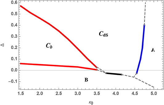
Figure 1. The CDT phase diagram. Phase transition between phase C_dS and C_b is (most likely) second order, as is the transition between C_b and B, while the transition between C_dS and A is first order. The transition between C_dS and B is still under investigation, but preliminary results suggest a first-order transition.

3.3. Observables and the UV Limit

What kind of observables can we use in CDT in search of a UV fixed point? We have no fields we can associate with lattice vertices or the centers of (sub)-simplices¹¹. However, we have geometric quantities, like the Regge curvature which is assigned to two-dimensional sub-simplices in the four-dimensional triangulation, and we also have the trivial field “1(n),” which assigns the real number 1 to each four-simplex and which turns out to be quite useful¹². At the same time, for any given geometry we can talk about geodesic distances between vertices or (sub)-simplices. This can be transferred to the quantum gravity theory in the path integral formalism, where one can talk about correlations between some of these quantities when they are separated by a certain geodesic distance. The subtlety lies in the fact that this distance has to be fixed outside the path integral, since we are integrating over geometries that define what we mean by distance. We will return to this point in section 4. Here we will use it in a specific CDT context where the situation is simpler. CDT is special because we have a time foliation, which on the lattice becomes an explicit time coordinate, namely, the n^t labeling of the various time-slices. In this sense the set-up in CDT is precisely the lattice set-up one would use in proper-time gauge in Hořava-Lifshitz gravity (HLG) [42, 43], although the presence of a preferred time in CDT is not associated with a breaking of four-dimensional diffeomorphism invariance (see [4] for a related discussion).

Let us introduce the notation 〈${O}$〉_N4 for a quantity ${O}$. It signifies the average of the quantity ${O}$, calculated using the partition function (15), but for fixed discrete four-volume N₄. (In practice the “calculation” means that we are performing MC simulations.) Now we can define the CDT version of (4) for the trivial field ϕ(n) = 1:

$\begin{array}{ll}{N}_3(n^t)=\frac{1}{2}{\displaystyle \sum _{\overrightarrow{n}(n^t)}}(1+1).& (16)\end{array}$

The notation is as follows: each time-slice is assigned a lattice time n^t. On this time-slice each three-simplex (tetrahedron) is assigned a label $\overrightarrow{n}(n^t)$ by analogy with the notation for the hypercubic lattice in Equation (4). This notation is only symbolic, since the three-dimensional triangulations are not regular and different time-slices need not contain the same number of three-simplices $N_3(n^t)$. Each of these three-simplices belongs to precisely two (4,1)-simplices, whose trivial fields “1” are represented in the sum in (16), and we divide by 2 to obtain $N_3(n^t)$. On a regular lattice, this number is of course trivial and fixed, but here it can vary, as mentioned, and becomes a dynamical variable. We now calculate averages and correlation functions like in (5), i.e., we calculate

$\begin{array}{ll}{\langle N_3(n^t)\rangle }_{N_4}& (17)\end{array}$

and

$\begin{array}{ll}{\langle N_3(n_1^t)N_3(n_2^t)\rangle }_c={\langle N_3(n_1^t)N_3(n_2^t)\rangle }_{N_4}-{\langle N_3(n_1^t)\rangle }_{N_4}{\langle N_3(n_2^t)\rangle }_{N_4}.& (18)\end{array}$

Figure 2 shows the average of $N_3(n^t)$ over many configurations in the case where the topology of the spatial slices is that of S³. It also shows the size of the fluctuations, i.e., it is a plot of $\langle N_3(n^t)\rangle$ and $\delta N_3(n^t)=\sqrt{{\langle N_3^2(n^t)\rangle }_c}$ from (17) and (18). In the region where $\langle N_3(n^t)\rangle >100$, the curve in Figure 2 fits perfectly to the functional form

$\begin{array}{ll}{N}_3^{cl}(n^t):\; =\langle N_3(n^t)\rangle =N_4\frac{3}{4\omega N_4^{1/4}}{cos}^3\left(\frac{n^t}{\omega N_4^{1/4}}\right),& (19)\end{array}$

where ω depends on κ₀ and Δ. Despite the fact that no background geometry enters into the path integral, a background volume profile appears to emerge. It is identical to a (Euclidean) de Sitter universe volume profile and the configurations created by the MC simulations can be viewed as quantum geometries that fluctuate around this background. While this is very interesting¹³, our main question here is whether we can use (17) and (18) to follow a path in the bare coupling constant space (κ₀, Δ) toward a UV fixed point in the same way as for the ϕ⁴-theory. More precisely, we want to identify physical observables. Since we can perform the MC simulations for various finite volumes N₄, we want to use finite-size scaling to identify a possible UV fixed point.

FIGURE 2

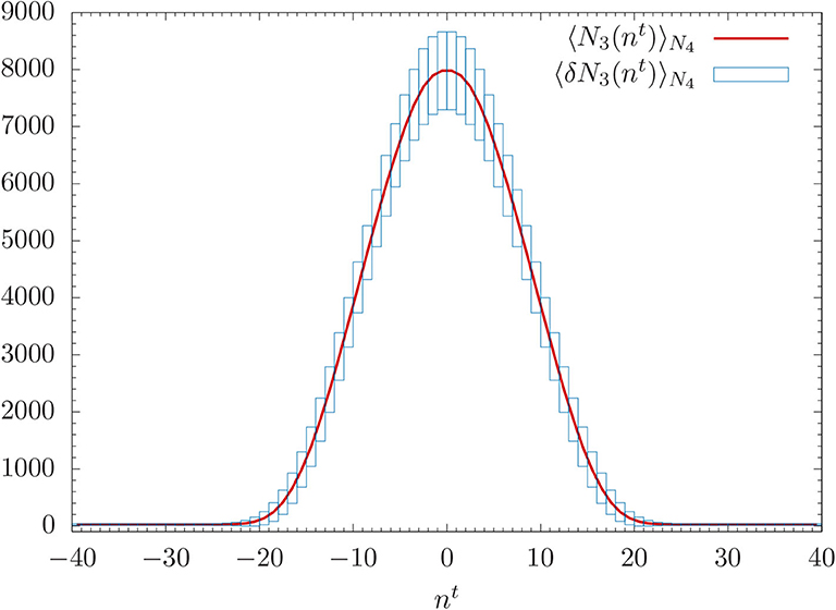
Figure 2. The average spatial volume ${\langle N_3(n^t)\rangle }_{N_4}$ as a result of MC measurements for N₄ = 362.000. The best fit (19) yields indistinguishable curves at given plot resolution. The bars indicate the average size of quantum fluctuations $\delta N_3(n^t)$.

A few starting remarks are in order. We have replaced a real field ϕ(n) with 1(n) in (16) and (18). Thus we cannot necessarily expect an exponential fall-off and a corresponding correlation length ξ like in (5). However, in the solvable two-dimensional models of both CDT and DT one does find an exponential fall-off related to the field 1(n) [45, 46]. This fall-off is related to the cosmological constants of the models, and the “mass” goes to zero with a vanishing cosmological constant. In four-dimensional gravity we expect massless gravitons (and thus maybe no exponential fall-off), but as shown in [41], there are terms in an effective continuum action of quantum gravity, which can lead to such an exponential fall-off, e.g., the non-local term

$\begin{array}{ll}{\Gamma }^{NL}=-\frac{b^2}{96\pi G}{\displaystyle \int }{d}^{4}x\sqrt{g}R\frac{1}{{\Delta }_g^2}R,& (20)\end{array}$

where Δ_g is the scalar Laplacian defined in the geometry related to the metric g_ij(x). Expanding the fluctuations to quadratic order around flat spacetime, b will appear as a mass term. We might observe such terms in case of toroidal topology, where the fluctuations we observe seem to be around flat spacetime. If the spatial topology is S³, the contributions from a term like (20) would mix with contributions from the cosmological term via the curvature of the background geometry used for S³. Thus, there might be a number of sources for an exponential fall-off of the (spatial) volume-volume correlator.

Equation (19) shows that for fixed κ₀ and Δ we have a well-defined scaling with N₄. The same is true for the volume-volume correlator, where the MC data (for spatial topology S³) is consistent with the formula

$\begin{array}{ll}{\langle N_3(n_1^t)N_3(n_2^t)\rangle }_c={\gamma }^2{N}_{4}F(\frac{n_1^t}{\omega N_4^{1/4}},\frac{n_2^t}{\omega N_4^{1/4}}),& (21)\end{array}$

$\begin{array}{ll}\sqrt{{\langle N_3^2(n^t)\rangle }_c}=\gamma \sqrt{N_4}G\left(\frac{n^t}{\omega N_4^{1/4}}\right).& (22)\end{array}$

Here γ depends on κ₀ and Δ. F is some scaling function which only depends slightly on κ₀ and Δ, and $G=\sqrt{F}$. Unfortunately, we cannot really use Equation (21) to extract a correlation length ξ independent of N₄. If any ξ could be associated with the correlator, it would already be “maximal,” i.e., of order ωN^1/4, the whole average time-length of the universe, without any fine-tuning of the bare coupling constants. A condition like (11) then becomes empty¹⁴ and we thus have to find other measures to keep continuum physics constant, when taking the lattice spacing to zero.

Figure 2 is for a specific value of N₄ and, as remarked above, we already have a scaling for fixed values of the bare coupling constants κ₀ and Δ. Equations (19), (21), and (22) are these scaling formulas. We see that the height of $\langle N_3(n^t)\rangle$ will grow as $N_4^{3/4}$, while the fluctuations only grow as $N_4^{1/2}$. For fixed (κ₀, Δ) in phase C_dS, the fluctuations will thus decrease relative to the volume for N₄ → ∞. The interpretation of this is that for fixed κ₀ and Δ the limit N₄ → ∞ is one where $V_4=N_4{a}^4$ goes to infinity while a stays constant.

An attempt to replace the ϕ⁴-observables (m_R, λ_R) with geometrical observables is the following. The physical volume of spacetime is $V_4=N_4{a}^4$. Similarly, the volume of a time-slice is $V_3(t)=\langle N_3(n^t)\rangle a^3$, t = n^ta. Let us attempt to take a continuum limit where V₄ and V₃(t) are finite, while N₄ → ∞. Such a limit would force a → 0, which is what we want. How do we ensure that N₄ → ∞ forces a → 0? For the scalar field we had the correlation length ξ and m_R which monitored a(ξ). Here we will insist that the relative size of V₃(t) and the quantum fluctuations δV₃(t) stay unchanged if we scale N₄ → ∞. This would be expected if V₃(t) can be interpreted as a physical continuum three-volume in the limit N₄ → ∞. Thus we require that (for sufficiently large N₄)

$\begin{array}{ll}\frac{\sqrt{{({\langle N_3^2(n^t)\rangle }_c)}_{N_4}}}{{\langle N_3(n^t)\rangle }_{N_4}}=\frac{\delta V_3(t)}{V_3(t)},\text{\hspace{1em}independent of }{N}_4.& (23)\end{array}$

From (19) and (22) this requirement implies that

$\begin{array}{ll}\omega ({\kappa }_0,\Delta )\gamma ({\kappa }_0,\Delta )=\text{const.}{N}_4^{1/4}.& (24)\end{array}$

ω and γ are constants independent of N₄ for fixed κ₀ and Δ. Starting out with some (κ₀, Δ) and a four-volume N₄(0) in phase C_dS, and then increasing N₄ will force us to change (κ₀, Δ) if (24) is to be fulfilled. Continuing to increase N₄ will trace out a path in the (κ₀, Δ)-coupling constant plane, and the endpoint for N₄ → ∞ will be a candidate for a UV fixed point.

The coupling constant flow related to (24) was investigated in [47] and the conclusion was like in the ϕ⁴-case. There seems to be no starting point in phase C_dS which leads to a curve where N₄ → ∞. In fact, while both ω and γ change somewhat when changing the coupling constants, their product does not change much. We conclude that this particular renormalization group analysis has not led us to a UV fixed point candidate. But even stronger, Equation (23) expresses the simple requirement that if we have a continuum universe of a certain size, it will have quantum fluctuations of a certain size. However, our model does not meet this requirement when we relate discretized and continuum variables in the most natural and simple-minded way.

There are a number of possible interpretations of this result. Firstly, on the technical side, since the analysis in [47] was made, we have obtained a better understanding of the phase diagram. At the time of the analysis in [47] phase C_dS was assumed to extend all the way down to phase B. Currently the most promising phase transition line for a higher-order transition is the C_dS-C_b transition line, and the endpoint of that transition line in particular. We now have a chance to approach this fixed point in an easier way using toroidal spatial topology. This is presently being explored. Secondly, we may be thinking of the quantum universe in the wrong way. In our reasoning we are applying some standard logic related to fluctuations to a macroscopic quantity like the three-volume of the universe. Maybe that is wrong. On the other hand, we have tried to estimate the size of the quantum universes by constructing the effective action for the three-volume, and comparing with mini-superspace expressions. The universes are estimated to have linear sizes not larger than 20 Planck lengths [3] for the N₄-values we are using. Therefore, a picture like that of Figure 2 should be correct: for a continuum universe of this size we expect significant quantum fluctuations. Thirdly, although we tried to emulate the flat-space quantum field theoretic way of looking for UV fixed points, we have not (yet) been able to identify a divergent correlation length, which is a crucial ingredient of the Wilsonian approach to quantum field theory and the renormalization group. It is the source of universality and dictates the way one moves from the regularized quantum field theory on the lattice to the continuum quantum field theory. There seems no reason that there should not be massless long-range excitations in a theory of gravity related to a universe like ours. However, it is much less clear what kind of excitations one would observe in a quantum universe of the size of 20 Planck lengths, and to what extent one can talk about scaling the lattice spacing a to zero compared to the Planck length. The estimates referred to above led to a lattice spacing of twice the Planck length. If these estimates can be trusted, our a is far from sub-Planckian. However, it is possible that the global conformal mode of the metric, whose effective behavior we are studying, is not well-suited for extracting a correlation length. In other words, it may not be possible to push the lattice spacing to a sub-Planckian region while maintaining an interpretation that is based on notions which are closely related to classical geometry, like “volume profiles.” The question of whether there is a correlation length in non-perturbative quantum gravity and whether its divergence relates to a UV phase transition therefore leads us to an even more basic question: what is “length” in quantum gravity, when in the path integral one integrates over the geometries that classically define the length? We turn to a discussion of this question in the next section.

4. Quantum Length

In ordinary quantum field theory, lengths and distances are defined with respect to a (flat) spacetime metric, which is part of the fixed background structure. One simply has

$\begin{array}{ll}\langle \varphi (x)\varphi (y)\rangle =f(|x-y|),& (25)\end{array}$

where |x − y| is the invariant spacetime distance between the spacetime points x and y. When trying to define correlation functions like (25) rigorously, e.g., on the lattice as in (2), one may have to rescale fields, coupling constants and the lattice spacing in order to obtain a finite continuum result, but the geodesic distance |x − y| in (Euclidean) spacetime is not touched. The situation is similar when we generalize to quantum field theory on a fixed, curved background. The analog of the two-point function (25) will still depend on the geodesic distance between x and y, but also on other coordinate-independent quantities involving the fixed spacetime geometry.

Moving on to quantum gravity, the path integral will contain an integration over geometries, in addition to the integration over field configurations. For these geometries, the geodesic distance between x and y will vary, as will the curvature invariants associated with a given geometry. In the absence of any a priori given background geometry, the only way in which a dependence on a distance (or other geometric invariants) could reappear in some propagator would be with respect to some “effective” or “emergent” geometry, generated by the quantum dynamics, and accompanied by quantum fluctuations¹⁵. The propagator should also reflect this to some approximation, depending on the size the geometric fluctuations. Such an “emergence” of a class of dominant geometries is what one observes in the MC simulations of CDT¹⁶ in phase C_dS.

For reference, let us examine the situation in two-dimensional quantum gravity, which we have argued is in some sense maximally “quantum.” Suppose we have a universe with the topology of a cylinder, where we fix the lengths of the two boundaries to L and the area (the spacetime volume) to A. For suitable values of L and A there will be a “minimal-area surface” with constant negative curvature between the two boundaries. Could this nice, classical geometry be the one that dominates the path integral, such that the integration over geometries could be approximated by considering only small fluctuations around it? It turns out that the answer is no. However, if two-dimensional gravity is coupled to a conformal field theories with a large negative central charge the answer is yes.

Whichever the case may be in four dimensions, some invariant notation of length or distance is clearly needed in the quantum theory to construct any meaningful propagators or n-point functions. Again, two-dimensional quantum gravity may provide some guidance for how to proceed. When discussing a quantum-gravitational generalization of (25), we used coordinates x and y to label spacetime points, while emphasizing the arbitrariness of this choice. In the context of non-perturbative quantum gravity it is more convenient to base the construction of invariant correlators on the notion of distance instead. Thus, we integrate only over geometries where x and y are separated precisely by a geodesic distance D. Equivalently, for a given geometry and a given x, we average in the matter functional integral over all points y which are separated a given distance D from x, and then integrate over all geometries. In this way we obtain a correlation function G_ϕ(x, D), which explicitly depends on what one could call the quantum distance D. Generalizing (2), its definition is

$\begin{array}{l}{G}_{\varphi }(x,D):\; =\\ \frac{\int {D}\left[g_{\mu \nu }\right]{\text{e}}^{-S\left[g\right]}\int {{D}}_g\varphi {\text{e}}^{-S\left[g,\varphi \right]}\int \text{d}y\sqrt{g(y)}\varphi (x)\varphi (y)\delta (D_g(x,y)-D)}{\int {D}\left[g_{\mu \nu }\right]{\text{e}}^{-S\left[g\right]}\int {{D}}_g\varphi {\text{e}}^{-S\left[g,\varphi \right]}},& (26)\end{array}$

where D_g(x, y) denotes the geodesic distance between x and y in the geometry with metric g_μν(x). Even in two-dimensional quantum gravity, the expression (26) is too complicated to compute analytically for a scalar field ϕ(x). However, for ϕ(x) = 1 – the “trivial” field we considered for CDT in section 3—one can in the DT formalism write down a lattice version of (26), solve analytically for the lattice propagator, and take the continuum limit where the lattice spacing goes to zero [45, 48]. After the continuum limit has been taken one finds

$\begin{array}{ll}{G}_1(x,D)\propto D^{3}F(D/V^{1/4}),F(x)=1+O(x^4),& (27)\end{array}$

if one fixes the spacetime volume to be V. Equation (27) shows that the quantum length D is very “quantum,” since it has an anomalous dimension, which moreover is related to the fractal dimension 4 of the quantum spacetime. If we set ϕ(y) = 1 in (26), the integral over y is the total volume (in this case the total length) of all points at geodesic distance D from x, forming a “spherical shell” S_x(D). For a smooth classical d-dimensional geometry we expect $S_x(D)\propto D^{d-1}$ for D sufficiently small. Here we find instead

$\begin{array}{ll}{G}_1(x,D)=\langle S_x(D)\rangle \propto D^3\text{\hspace{1em}for\hspace{1em}}D\ll V^{1/4},& (28)\end{array}$

which shows that the fractal dimension of two-dimensional Euclidean quantum spacetime is 4. The important point here is that the distance or length has become a quantum operator, which is natural in a theory of quantum geometry. Since the geodesic distance is a very complicated non-local quantity, it is remarkable that the quantum average of this quantity, defined in Equation (26) for ϕ(x) = 1, has a non-trivial well-defined scaling dimension. However, its noncanonical value implies a nonstandard scaling behavior of the quantum geodesic distance D in the regularized DT-lattice theory for a spacetime volume $V=N_2{a}^2$, where N₂ counts the number of triangles in the triangulation. Namely, in a continuum limit where V stays finite and N₂ → ∞ (and thus a → 0), D on average involves only a number of links $\propto 1/\sqrt{a}$. This is very different from the generic situation in the ϕ⁴-theory, where linear distance in the continuum limit would scale ∝1/a. In the ϕ⁴-lattice scenario a behavior $\propto 1/\sqrt{a}$ would correspond to zero length in the continuum limit. However, it is possible and nontrivial on the DT lattices because of the fractal structure of a generic triangulation.

Another related example where distances become quantum comes from bosonic string theory, although in a string-theoretical context it is usually not presented this way. Bosonic string theory in d dimensions can be viewed as a theory of two-dimensional quantum gravity with coordinates (ω₁, ω₂) on the world sheet, coupled to d scalar fields $X^i({\omega }_1,{\omega }_2)$, taking values in the target space R^d. Let us consider closed strings, and the so-called tree-amplitude for the two-point function. This is calculated by considering two infinitesimal loops separated by a distance D in target space, summing in the path integral over all surfaces $X^i({\omega }_1,{\omega }_2)$ with cylinder topology in target space, with these loops as boundaries, weighted by the string action. One way to carry out this calculation is to find the classical string solution $X_{\text{cl}}^i({\omega }_1,{\omega }_2)$ with the given boundaries, perform a split

$\begin{array}{ll}{X}^i=X_{\text{cl}}^i+X_{\text{q}}^i& (29)\end{array}$

and integrate over the quantum fields $X_{\text{q}}^i$. Just like in standard quantum field theory, this integration will in general require a regularization. In addition, to obtain a finite effective action, $X_{\text{cl}}^i$ will need a wave function renormalization. However, the distance D appears as a parameter in $X_{\text{cl}}^i$ and the wave function renormalization of $X_{\text{cl}}^i$ in reality becomes a renormalization of the distance D in target space, as shown in detail in [49, 50]. Like in the case of pure two-dimensional quantum gravity mentioned above, the need for a renormalization of the distance D can be related to a fractal structure, in this case, the fractal structure of the random surfaces embedded in R^d [49, 50].

The lesson to take away from this discussion is that unless some yardstick emerges alongside a “dominant” geometry in a non-perturbative path integral over geometries, or is provided by hand through suitable boundary conditions, a notion of (quantum) distance must be introduced in the Planckian regime. As the above examples illustrate, such notions can be found, but will typically behave nonclassically or even scale anomalously relative to the volume. Clearly, this needs to be taken into account when constructing and interpreting propagators and other geometric observables, for example, in a renormalization group analysis near a UV fixed point. Whether such a quantum length possesses a large-scale classical limit or can be promoted to a “physical” length needs to be investigated, and is certainly not a given.

5. Discussion

In the asymptotic safety scenario, quantum gravity is defined as an ordinary quantum field theory at a UV fixed point. We have shown here how one can in principle use computer simulations to search for such a fixed point, in close analogy with the search for a UV fixed point in a four-dimensional ϕ⁴-theory. The framework of CDT quantum gravity is well suited to try and verify the findings of the functional renormalization group analysis in the continuum independently. One particular correlation function, that of the spatial volume profile (equivalently, the global conformal mode of the spatial metric), has already been studied extensively, but so far no indication of a UV fixed point has been seen. There could be many reasons for this. Despite the compelling evidence from a body of work in the continuum theory [35–39, 51]¹⁷, such a fixed point may not exist, and the asymptotic safety scenario not realized as a way to define quantum gravity beyond perturbation theory. Defining trajectories of constant physics near the Planck scale through an observable that describes the global shape of the universe may be a wrong choice. As emphasized in [47], at the very least one would like to repeat the analysis in terms of other, more local observables. A new candidate may be the quantum Ricci curvature [52, 53], currently under investigation. Our assessment that the lattice version of δV₃(t) is too small and does not increase sufficiently when we move toward the C_dS-C_b phase transition line may be based on our incomplete understanding of how quantum length and volume behave near the Planck scale. Also, maybe we are not using an action which is general enough to localize the UV fixed point? We are using the Regge discretized version of the Einstein-Hilbert action with one additional deformation parameter Δ. From a continuum point of view one could think of adding all kind of higher curvature terms to the action. We have not done that for two reasons. The firstly, in the formalism of CDT there are no simple natural candidates for the higher curvature terms. The geometric Regge prescription only exists for the R-term, and attempts to put in by hand arbitrary ad hoc generalizations have not worked (see [54] for old attempts). Secondly, the functional renormalization group analysis sees clear evidence for a fixed point even if one truncates the effective action to contain only the Einstein-Hilbert term. From the lattice perspective the interpretation of this is that one should be able to get quite close to the fixed point by finetuning the two bare coupling constants κ₀ and Δ, even if we might not be able to reach all the way to the fixed point. However, it is disappointing that we have not really seen much sign of an approach to a fixed point, as we would have expected from the continuum renormalization group calculations. Another possibility that may be worthwhile exploring is that the quantum-geometric phase transitions in CDT are different from the more conventional Landau-type phase transitions where the Wilsonian renormalization group philosophy works so well. In particular, the C_dS-C_b transition may share traits with the topological phase transitions occurring in condensed matter physics [55, 56]. The transition is associated with the appearance of a localized structure in an otherwise seemingly homogeneous and isotropic universe. It was overlooked for a long time, since the order parameters that exhibit the transition are also of a non-standard nature with a strong topological flavor [33]. In addition, one has observed long auto-correlation times in the MC simulations at the C_dS-C_b transition, presumably caused by major rearrangements of the internal connectivity of the triangulations in connection with the symmetry breaking. This is again reminiscent of some features seen in topological phase transitions, some of which also have no clear divergent correlation lengths associated with them. How to relate such transitions to a UV fixed point in quantum gravity is an interesting challenge.

Data Availability Statement

The datasets generated for this study are available on request to the corresponding author.

Author Contributions

All authors listed have made a substantial, direct and intellectual contribution to the work, and approved it for publication.

Conflict of Interest

The authors declare that the research was conducted in the absence of any commercial or financial relationships that could be construed as a potential conflict of interest.

Acknowledgments

JA thanks Frank Saueressig for discussions. JA acknowledges support from the Danish Research Council grant Quantum Geometry, grant 7014-00066B. JG-S acknowledges support from the grant UMO-2016/23/ST2/00289 from the National Science Centre, Poland. AG acknowledges support by the National Science Centre, Poland, under grant no. 2015/17/D/ST2/03479. JJ acknowledges support from the National Science Centre, Poland, grant 2019/33/B/ST2/00589.

Footnotes

1. ^Using a description like this we assume we are so close to a continuum limit that we can use a continuum language for the observables, rather than referring explicitly to the lattice. In addition, note that a procedure like this will not leave all observables unchanged, but only the physical coupling constants. One could follow another renormalization procedure, where the action contained “all possible coupling constants.” In this space one could follow a path which leaves all observables invariant.

2. ^For a detailed discussion see the book [1].

3. ^A priori the β-function is a function of λ₀ and m₀a₀, but one can show that close to the fixed point one can ignore the m₀a₀-dependence.

4. ^If ${\lambda }_0^{*}=0$, we have a so-called Gaussian fixed point and the formula (10) has to be modified slightly.

5. ^In the parametrization chosen here, symmetry breaking can occur when we also allow negative values of the bare coupling constant $m_0^2$ in (1).

6. ^The continuum path integral over four-dimensional geometries has not yet been constructed in any mathematically rigorous way, but one expects that the geometries will include many “wild” geometries which are continuous but nowhere differentiable. In this sense the set of piecewise geometries proposed is a set of “nice” geometries.

7. ^It should be emphasized that it is a sum over geometries, not a sum over metrics g_ij defining a geometry. In a gauge theory this would correspond to a sum over equivalence classes of gauge fields, something one has only been able to dream about.

8. ^No coordinates were introduced at any point in the lattice theory, so agreement with a diffeomorphism-invariant theory means that all coordinate-invariant quantities which can be calculated agree.

9. ^We assume here that N₀ and N₄ are large, since the Euler characteristic of the closed manifold in principle also appears in (13), but is ignored.

10. ^Originally in CDT, Δ was associated with an asymmetry between the lengths of lattice links in the time direction and in the other directions.

11. ^One can in principle associate by hand a coordinate system to each simplex, compute transition functions between the different coordinate systems and assign metric tensor fields g_ij to each simplex, but this becomes very cumbersome and has so far not been useful in a DT or CDT context. It would also re-introduce a coordinate dependence which is clearly unwanted.

12. ^As observed in [41], if one assumes the existence of a time foliation and expands the general continuum effective action for quantum gravity to quadratic order, one obtains naturally a projection on the constant mode when integrating certain correlators over space, as we will do in (18) and as was done in (4) in flat spacetime. In this sense one is naturally led to 1(n) for such integrated correlators.

13. ^The dominant “semiclassical background geometries” seem to depend on the topology of space (as do classical solutions of Einstein's equations). If we change the topology of space from S³ to T³, the dominant volume profile will be constant. However, the phase diagram is unchanged [40, 44].

14. ^The situation might be different in the case of toroidal spatial topology, where the time extent of the universe is not dynamically adjusted to the total four-volume N₄. This is presently under investigation.

15. ^One can of course choose a fictitious “background” geometry and expand everything around it. But nothing can depend on this geometry, which implies that distances defined with respect to it will be as fictitious as the geometry itself.

16. ^To be precise, the emergence of classical behavior refers only to those aspects of geometry that are captured by the behavior in proper time t of the three volume V(t).

17. ^The calculation reported in [51] seems in particular to be close in spirit to the CDT approach.

References

1. Montvay I, Munster G. Quantum fields on a lattice. In: Cambridge Monographs on Mathematical Physics. Cambridge: Cambridge University Press (1997). doi: 10.1017/CBO9780511470783

CrossRef Full Text | Google Scholar

2. Lüscher M, Weisz P. Scaling laws and triviality bounds in the lattice ϕ⁴ theory. Nucl Phys B. (1987) 290:25. doi: 10.1016/0550-3213(87)90177-5

CrossRef Full Text | Google Scholar

3. Ambjorn J, Goerlich A, Jurkiewicz J, Loll R. Nonperturbative quantum gravity. Phys Rept. (2012) 519:127. doi: 10.1016/j.physrep.2012.03.007

CrossRef Full Text | Google Scholar

4. Loll R. Quantum gravity from causal dynamical triangulations: a review. Class Quant Grav. (2020) 37:013002. doi: 10.1088/1361-6382/ab57c7

CrossRef Full Text | Google Scholar

5. Regge T. General relativity without coordinates. Nuovo Cim. (1961) 19:558.

Google Scholar

6. Ambjorn J, Durhuus B, Jonsson T. Quantum Geometry. A Statistical Field Theory Approach. Cambridge, UK: Cambridge University Press (1997).

Google Scholar

7. Ambjorn J, Durhuus B, Frohlich J. Diseases of triangulated random surface models, and possible cures. Nucl Phys B. (1985) 257:433. doi: 10.1016/0550-3213(85)90356-6

CrossRef Full Text | Google Scholar

8. David F. Planar diagrams, two-dimensional lattice gravity and surface models. Nucl Phys B. (1985) 257:45. doi: 10.1016/0550-3213(85)90335-9

CrossRef Full Text | Google Scholar

9. Kazakov VA, Migdal AA, Kostov IK. Critical properties of randomly triangulated planar random surfaces. Phys Lett B. (1985) 157:295. doi: 10.1016/0370-2693(85)90669-0

CrossRef Full Text | Google Scholar

10. Knizhnik VG, Polyakov AM, Zamolodchikov AB. Fractal structure of 2D quantum gravity. Mod Phys Lett A. (1988) 3:819. doi: 10.1142/S0217732388000982

CrossRef Full Text | Google Scholar

11. David F. Conformal field theories coupled to 2D Gravity in the conformal gauge. Mod Phys Lett A. (1988) 3:1651. doi: 10.1142/S0217732388001975

CrossRef Full Text | Google Scholar

12. Distler J, Kawai H. Conformal field theory and 2D quantum gravity. Nucl Phys B. (1989) 321:509. doi: 10.1016/0550-3213(89)90354-4

CrossRef Full Text | Google Scholar

13. Fateev V, Zamolodchikov AB, Zamolodchikov AB. Boundary Liouville field theory. 1. Boundary state and boundary two point function. hep-th/0001012.

Google Scholar

14. Ambjorn J, Jurkiewicz J, Makeenko YM Multiloop correlators for two-dimensional quantum gravity. Phys Lett B. (1990) 251:517. doi: 10.1016/0370-2693(90)90790-D

CrossRef Full Text | Google Scholar

15. Ambjorn J, Jurkiewicz J. Four-dimensional simplicial quantum gravity. Phys Lett B. (1992) 278:42–50. doi: 10.1016/0370-2693(92)90709-D

CrossRef Full Text | Google Scholar

16. Agishtein ME, Migdal AA. Simulations of four-dimensional simplicial quantum gravity. Mod Phys Lett A. (1992) 7:1039. doi: 10.1142/S0217732392000938

CrossRef Full Text | Google Scholar

17. Agishtein ME, Migdal AA. Critical behavior of dynamically triangulated quantum gravity in four-dimensions. Nucl Phys B. (1992) 385:395. doi: 10.1016/0550-3213(92)90106-L

CrossRef Full Text | Google Scholar

18. Bialas P, Burda Z, Krzywicki A, Petersson B Focusing on the fixed point of 4-D simplicial gravity. Nucl Phys B. (1996) 472:293–308. doi: 10.1016/0550-3213(96)00214-3

CrossRef Full Text | Google Scholar

19. Catterall S, Renken R, Kogut JB. Singular structure in 4-D simplicial gravity. Phys Lett B. (1998) 416:274–80. doi: 10.1016/S0370-2693(97)01349-X

CrossRef Full Text | Google Scholar

20. Ambjorn J, Glaser L, Goerlich A, Jurkiewicz J. Euclidian 4D quantum gravity with a non-trivial measure term. J High Energy Phys. (2013) 1310:100. doi: 10.1007/JHEP10(2013)100

CrossRef Full Text | Google Scholar

21. Coumbe D, Laiho J. Exploring Euclidean dynamical triangulations with a non-trivial measure term. J High Energy Phys. (2015) 1504:028. doi: 10.1007/JHEP04(2015)028

CrossRef Full Text | Google Scholar

22. Ambjorn J, Jurkiewicz J, Loll R. Dynamically triangulating Lorentzian quantum gravity. Nucl Phys B. (2001) 610:347. doi: 10.1016/S0550-3213(01)00297-8

CrossRef Full Text | Google Scholar

23. Ambjørn J, Jurkiewicz J, Loll R. Reconstructing the universe. Phys Rev D. (2005) 72:064014. doi: 10.1103/PhysRevD.72.064014

CrossRef Full Text | Google Scholar

24. Ambjørn J, Jurkiewicz J, Loll R. Emergence of a 4-D world from causal quantum gravity. Phys Rev Lett. (2004) 93:131301. doi: 10.1103/PhysRevLett.93.131301

PubMed Abstract | CrossRef Full Text | Google Scholar

25. Ambjorn J, Görlich A, Jurkiewicz J, Loll R. The Nonperturbative quantum de sitter universe. Phys Rev D. (2008) 78:063544. doi: 10.1103/PhysRevD.78.063544

PubMed Abstract | CrossRef Full Text | Google Scholar

26. Ambjørn J, Görlich A, Jurkiewicz J, Loll R. Planckian birth of the quantum de sitter universe. Phys Rev Lett. (2008) 100:091304. doi: 10.1103/PhysRevLett.100.091304

PubMed Abstract | CrossRef Full Text | Google Scholar

27. Ambjorn J, Görlich A, Jordan S, Jurkiewicz J, Loll R. CDT meets Horava-Lifshitz gravity. Phys Lett B. (2010) 690:413. doi: 10.1016/j.physletb.2010.05.054

CrossRef Full Text | Google Scholar

28. Ambjorn J, Jordan S, Jurkiewicz J, Loll R. A second-order phase transition in CDT. Phys Rev Lett. (2011) 107:211303. doi: 10.1103/PhysRevLett.107.211303

PubMed Abstract | CrossRef Full Text | Google Scholar

29. Ambjorn J, Jordan S, Jurkiewicz J, Loll R. Second- and first-order phase transitions in CDT. Phys Rev D. (2012) 85:124044. doi: 10.1103/PhysRevD.85.124044

CrossRef Full Text | Google Scholar

30. Ambjorn J, Gizbert-Studnicki J, Görlich A, Jurkiewicz J, Németh D. Towards an UV fixed point in CDT gravity. J High Energy Phys. (2019) 1907:166. doi: 10.1007/JHEP07(2019)166

CrossRef Full Text | Google Scholar

31. Ambjorn J, Coumbe D, Gizbert-Studnicki J, Görlich A, Jurkiewicz J. Critical phenomena in causal dynamical triangulations. Class Quant Grav. (2019) 36:224001. doi: 10.1088/1361-6382/ab4184

CrossRef Full Text | Google Scholar

32. Ambjorn J, Coumbe D, Gizbert-Studnicki J, Gorlich A, Jurkiewicz J. New higher-order transition in causal dynamical triangulations. Phys Rev D. (2017) 95:124029. doi: 10.1103/PhysRevD.95.124029

CrossRef Full Text | Google Scholar

33. Ambjorn J, Gizbert-Studnicki J, Görlich A, Jurkiewicz J, Klitgaard N, Loll R. Characteristics of the new phase in CDT. Eur Phys J C. (2017) 77:152. doi: 10.1140/epjc/s10052-017-4710-3

PubMed Abstract | CrossRef Full Text | Google Scholar

34. Weinberg S. Ultraviolet divergences in quantum theories of gravitation. In: Hawking SW, Israel W, editors. General Relativity: Einstein Centenary Survey. Cambridge, UK: Cambridge University Press (1979). p. 790–831.

Google Scholar

35. Reuter M. Nonperturbative evolution equation for quantum gravity. Phys Rev D. (1998) 57:971–85.

Google Scholar

36. Codello A, Percacci R, Rahmede C. Investigating the ultraviolet properties of gravity with a Wilsonian renormalization group equation. Ann Phys. (2009) 324:414. doi: 10.1016/j.aop.2008.08.008

CrossRef Full Text | Google Scholar

37. Reuter M, Saueressig F. Functional renormalization group equations, asymptotic safety, and quantum Einstein gravity. In Ocampo H, Pariguan E, and Paycha S, editors. Geometric and Topological Methods for Quantum Field Theory. Cambridge: Cambridge University Press (2007). p. 288–329. doi: 10.1017/CBO9780511712135.008

PubMed Abstract | CrossRef Full Text | Google Scholar

38. Niedermaier M, Reuter M. The asymptotic safety scenario in quantum gravity. Living Rev Rel. (2006) 9:5. doi: 10.12942/lrr-2006-5

PubMed Abstract | CrossRef Full Text | Google Scholar

39. Litim DF. Fixed points of quantum gravity. Phys Rev Lett. (2004) 92:201301. doi: 10.1103/PhysRevLett.92.201301

PubMed Abstract | CrossRef Full Text | Google Scholar

40. Ambjorn J, Gizbert-Studnicki J, Görlich A, Jurkiewicz J, Nmeth D. The phase structure of Causal Dynamical Triangulations with toroidal spatial topology. J High Energy Phys. (2018) 1806:111. doi: 10.1007/JHEP06(2018)111

CrossRef Full Text | Google Scholar

41. Knorr B, Saueressig F. Towards reconstructing the quantum effective action of gravity. Phys Rev Lett. (2018) 121:161304. doi: 10.1103/PhysRevLett.121.161304

PubMed Abstract | CrossRef Full Text | Google Scholar

42. Hořava P. Quantum gravity at a Lifshitz point. Phys Rev D. (2009) 79:084008. doi: 10.1103/PhysRevD.79.084008

PubMed Abstract | CrossRef Full Text | Google Scholar

43. Hořava P, Melby-Thompson CM. General covariance in quantum gravity at a Lifshitz point. Phys Rev D. (2010) 82:064027. doi: 10.1103/PhysRevD.82.064027

CrossRef Full Text | Google Scholar

44. Ambjorn J, Gizbert-Studnicki J, Görlich A, Grosvenor K, Jurkiewicz J. Four-dimensional CDT with toroidal topology. Nucl Phys B. (2017) 922:226. doi: 10.1016/j.nuclphysb.2017.06.026

CrossRef Full Text | Google Scholar

45. Ambjorn J, Watabiki Y. Scaling in quantum gravity. Nucl Phys B. (1995) 445:129. doi: 10.1016/0550-3213(95)00154-K

CrossRef Full Text | Google Scholar

46. Ambjorn J, Loll R. Nonperturbative Lorentzian quantum gravity, causality and topology change. Nucl Phys B. (1998) 536:407. doi: 10.1016/S0550-3213(98)00692-0

CrossRef Full Text | Google Scholar

47. Ambjorn J, Görlich A, Jurkiewicz J, Kreienbuehl A, Loll R. Renormalization group flow in CDT. Class Quant Grav. (2014) 31:165003. doi: 10.1088/0264-9381/31/16/165003020

CrossRef Full Text | Google Scholar

48. Ambjorn J, Jurkiewicz J, Watabiki Y. On the fractal structure of two-dimensional quantum gravity. Nucl Phys B. (1995) 454:313. doi: 10.1016/0550-3213(95)00468-8

CrossRef Full Text | Google Scholar

49. Ambjorn J, Makeenko Y. Stability of the nonperturbative bosonic string vacuum. Phys Lett B. (2016) 756:142. doi: 10.1016/j.physletb.2016.02.075

CrossRef Full Text | Google Scholar

50. Ambjörn J, Makeenko Y. Scaling behavior of regularized bosonic strings. Phys Rev D. (2016) 93:066007. doi: 10.1103/PhysRevD.93.066007

CrossRef Full Text | Google Scholar

51. Contillo A, Rechenberger S, Saueressig F. Renormalization group flow of Hořava-Lifshitz gravity at low energies. J High Energy Phys. (2013) 1312:017. doi: 10.1007/JHEP12(2013)017

CrossRef Full Text | Google Scholar

52. Klitgaard N, Loll R. Implementing quantum Ricci curvature. Phys Rev D. (2018) 97:106017. doi: 10.1103/PhysRevD.97.106017

CrossRef Full Text | Google Scholar

53. Klitgaard N, Loll R. Introducing quantum ricci curvature. Phys Rev D. (2018) 97:046008. doi: 10.1103/PhysRevD.97.046008

CrossRef Full Text | Google Scholar

54. Ambjorn J, Jurkiewicz J, Kristjansen CF. Quantum gravity, dynamical triangulations and higher derivative regularization. Nucl Phys B. (1993) 393:601–32. doi: 10.1016/0550-3213(93)90075-Z

CrossRef Full Text | Google Scholar

55. Lutchyn RM, Sau JD, Sarma SD. Majorana fermions and a topological phase transition in semiconductor-superconductor heterostructures. Phys Rev Lett. (2010) 105:077001. doi: 10.1103/PhysRevLett.105.077001

CrossRef Full Text | Google Scholar

56. Chen X, Zheng-Cheng G, Xiao-Gang W. Local unitary transformation, long-range quantum entanglement, wave function renormalization, and topological order. Phys Rev B. (2010) 82:155138. doi: 10.1103/PhysRevB.82.155138

CrossRef Full Text | Google Scholar