Bifurcation and Numerical Simulations of Ca2+ Oscillatory Behavior in Astrocytes

Introduction

Ca²⁺ as an important second messenger in the cytosol is critical for synaptic neurons and glia cells in the brain [1]. The oscillatory changes in concentration of Ca²⁺ are called Ca²⁺ oscillations and play an active part in the transmission of chemical and electrical signaling process [2]. Astrocytes comprise approximately 50% of the volume of human brain and exhibit not only neuron-dependent Ca²⁺ oscillations but also spontaneous Ca²⁺ waves [3]. It was demonstrated that the frequencies and amplitudes of Ca²⁺ oscillations play key roles in Ca²⁺ signal transduction in the nervous system [4]. Recent results from experiment calcium release-activated calcium channel (CRAC) have shown that it is effective for the control in inhibiting neuronal excitability by enhancing calcium release from astrocytes [5].

It was generally considered that Ca²⁺ oscillations in astrocyte take place in response to external stimuli, inducing the release of neuro-active chemicals [6, 7]. This view began to change as several lines of evidence indicate that these oscillations can also be formed spontaneously [8]. Nevertheless, the mechanism and functional role involved in these stochastic spontaneous Ca²⁺ waves are still not well-understood. Basically, Ca²⁺ signal transmission of astrocytes in the brain may vary owing to certain bifurcation principles, and different chemical information is typically characterized by frequency, amplitude, and spatial Ca²⁺ propagation [9]. Dynamical mechanisms that underlie the Ca²⁺ waves have been investigated from both theoretical and experimental points of view in recent years [10–18]. Therefore, the stability and bifurcation analysis are fundamental to investigate the appearance and disappearance of spontaneous Ca²⁺ oscillations in astrocytes. In the last decades, existing mathematical models helped explore the possible dynamical mechanism of these oscillatory activities in neuronal excitability [19–23].

Stability of Equilibrium Point and Bifurcation Analysis

In the present work, we apply an extension of the one-pool model proposed by Lavrentovich and Hemkin as a specific example of the stability of equilibrium point and the bifurcation scenario. This model consists of three main variables: cytosol Ca²⁺ concentration (Ca_cyt), Ca²⁺ concentration in the endoplasmic reticulum (Ca_er), and IP₃ concentration in cell (IP₃). The equations and meanings of each expression in the model are given as follows:

$\begin{array}{ll}\{\begin{array}{c}\frac{dC{a}_{\text{cyt}}}{dt}=v_{in}-k_{\text{out}}C{a}_{\text{cyt}}+v_{\text{CICR}}-v_{\text{serca}}+k_f\left(C{a}_{\text{er}}-C{a}_{\text{cyt}}\right),\hfill \\ \frac{dC{a}_{\text{er}}}{dt}=v_{\text{serca}}-v_{CICR}-k_f\left(C{a}_{\text{er}}-C{a}_{\text{cyt}}\right),\hfill \\ \frac{dI{P}_3}{dt}=v_{\text{PLC}}-k_{\text{deg}}{IP}_3,\hfill \end{array}\hfill & (1)\end{array}$

where

$\begin{array}{l}{v}_{\text{serca}}=v_{M2}\left(\frac{C{a}_{\text{cyt}}^2}{C{a}_{\text{cyt}}^2+k_2^2}\right),\\ V_{\text{PLC}}=v_p\left(\frac{C{a}_{\text{cyt}}^2}{C{a}_{\text{cyt}}^2+k_p^2}\right),\\ v_{\text{CICR}}=4v_{M3}\left(\frac{k_{\text{CaA}}^{n}C{a}_{\text{cyt}}^n}{\left(C{a}_{\text{cyt}}^n+k_{\text{CaA}}^n\right)\left(C{a}_{\text{cyt}}^n+k_{\text{CaI}}^n\right)}\right)\\ \times \left(\frac{I{P}_3^m}{I{P}_3^m+k_{\text{ip}3}^m}\right)\left(C{a}_{\text{er}}-C{a}_{\text{cyt}}\right).\end{array}$

The details of each parameter can be found in Table 1 and [4].

TABLE 1

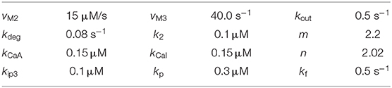
Table 1. Model parameters for which all results are computed unless otherwise stated.

Analysis of Stability and Bifurcation of Equilibria

In the following, v_in is chosen as the bifurcation parameter, corresponding to Ca²⁺ inflow into the cytosol through the astrocyte's membrane.

For convenience, let x = Ca_cyt, y = Ca_er, z = IP₃, and r = v_in, we first rewrite model (1) as the following form:

$\begin{array}{ll}\{\begin{array}{c}\stackrel{.}{x}=r-x+0.5y-\frac{15x^2}{x^2+0.01}-\frac{3.466x^{2.02}{z}^{2.2}(x-y)}{(x^{2.02}+0.022)(z^{2.2}+0.0063)},\hfill \\ \stackrel{.}{y}=0.5x-0.5y+\frac{15x^2}{x^2+0.01}+\frac{3.466x^{2.02}{z}^{2.2}(x-y)}{(x^{2.02}+0.022)(z^{2.2}+0.0063)},\hfill \\ \stackrel{.}{z}=\frac{0.05x^2}{x^2+0.09}-0.08z.\hfill \end{array}\hfill & (2)\end{array}$

The equilibrium of system (2) meets the following equations:

$\begin{array}{ll}\{\begin{array}{c}x=\frac{r}{k_{\text{out}}}\hfill \\ z=\frac{v_{\text{p}}{x}^2}{(x^2+k_{\text{p}}^2)k_{\text{deg}}}\hfill \\ y=\frac{v_{\text{serca}}-v_{\text{CICR}}+k_{\text{f}}x}{k_{\text{f}}}\hfill \end{array}\hfill & (3)\end{array}$

Let x₀, y₀, and z₀ be the roots of Equation (2) and x₁ = x – x₀, y₁ = y – y₀, and z₁ = z – z₀, we have the following representations:

$\begin{array}{ll}\{\begin{array}{c}{\stackrel{.}{x}}_1=r-(x_1+x_0)+0.5\left(y_1+y_0\right)-\frac{15{(x_1+x_0)}^2}{{(x_1+x_0)}^2+0.01}-\hfill \\ \frac{3.466{(x_1+x_0)}^{2.02}{(z_1+z_0)}^{2.2}(x_1+x_0-y_1-y_0)}{\left({(x_1+x_0)}^{2.02}+0.022\right)\left({(z_1+z_0)}^{2.2}+0.0063\right)},\hfill \\ {\stackrel{.}{y}}_1=0.5(x_1+x_0)-0.5\left(y_1+y_0\right)+\frac{15{(x_1+x_0)}^2}{{(x_1+x_0)}^2+0.01}\hfill \\ +\frac{3.466{(x_1+x_0)}^{2.02}{(z_1+z_0)}^{2.2}\left(x_1+x_0-y_1-y_0\right)}{\left({(x_1+x_0)}^{2.02}+0.022\right)\left({(z_1+z_0)}^{2.2}+0.0063\right)},\hfill \\ {\stackrel{.}{z}}_1=\frac{0.05{(x_1+x_0)}^2}{{(x_1+x_0)}^2+0.09}-0.08(z_1+z_0).\hfill \end{array}\hfill & (4)\end{array}$

The corresponding equilibrium is (0, 0, 0), and system (4) has the same properties with the equilibrium of system (2). With simple calculation, it is easy to calculate the Jacobian matrix of system (4),

$\begin{array}{l}A\; ={(a_{ij})}_{3\times 3}=\left(\begin{array}{ccc}{a}_{11}& a_{12}& a_{13}\\ a_{21}& a_{22}& a_{23}\\ a_{31}& a_{32}& a_{33}\end{array}\right),\end{array}$

where

$\begin{array}{l}{a}_{11}=\frac{30x^3}{{\left(x^2+0.01\right)}^2}-\frac{30}{x^2+0.01}-\frac{3.465966x^{2.02}{z}^{2.2}}{\sigma }\\ -\frac{7.0012517x^{1.02}{z}^{2.2}\left(x-y\right)}{\sigma }+\frac{14.002503x^{3.04}{z}^{2.2}\left(x-y\right)}{\sigma \left(x^{2.02}+0.021622\right)}-1,\\ a_{12}=\frac{3.465966x^{2.02}{z}^{2.2}}{\sigma }+0.5,\\ a_{13}=\frac{7.6251256x^{2.02}{z}^{3.4}\left(x-y\right)}{\sigma \left(z^{2.2}+0.00630957\right)}-\frac{7.625125x^{2.02}{z}^{1.2}\left(x-y\right)}{\sigma },\\ a_{21}=-\frac{30x^3}{{\left(x^2+0.01\right)}^2}+\frac{30}{x^2+0.01}+\frac{3.465966x^{2.02}{z}^{2.2}}{\sigma }\\ +\frac{7.0012517x^{1.02}{z}^{2.2}\left(x-y\right)}{\sigma }-\frac{14.002503x^{3.04}{z}^{2.2}\left(x-y\right)}{\sigma \left(x^{2.02}+0.021622\right)}+0.5,\end{array}$

$\begin{array}{l}{a}_{22}=-\frac{3.465966x^{2.02}{z}^{2.2}}{\sigma }-0.5,\\ a_{23}=-\frac{7.6251256x^{2.02}{z}^{3.4}\left(x-y\right)}{\sigma \left(z^{2.2}+0.00630957\right)}+\frac{7.625125x^{2.02}{z}^{1.2}\left(x-y\right)}{\sigma },\\ a_{31}=\frac{0.1x}{x^2+0.09}-\frac{0.1x^3}{{\left(x^2+0.09\right)}^2},\\ a_{32}=0,\\ a_{33}=-0.8,\\ \sigma ={\left(x^{2.02}+0.02166228\right)}^2\left(z^{2.2}+0.0063095\right).\end{array}$

And one can easily obtain the following characteristic equation:

$\begin{array}{l}{\lambda }^3+Q_3{\lambda }^2+Q_2\lambda +Q_1=0,\end{array}$

where

$\begin{array}{l}{Q}_1=-(a_{11}+a_{22}+a_{33}),\\ Q_2=a_{11}{a}_{22}+a_{11}{a}_{33}+a_{22}{a}_{33}-a_{13}{a}_{31}-a_{12}{a}_{21}-a_{32}{a}_{23},\\ Q_3=a_{31}{a}_{13}{a}_{22}+a_{12}{a}_{21}{a}_{33}+a_{32}{a}_{23}{a}_{11}-a_{11}{a}_{22}{a}_{33}\\ -a_{12}{a}_{23}{a}_{31}-a_{13}{a}_{21}{a}_{32}.\end{array}$

After a simple calculation, we have the following equations:

$\begin{array}{l}{Q}_1=\frac{30x}{x^2+0.01}-\frac{30x^3}{{\left(x^2+0.01\right)}^2}+\frac{6.93193x^{2.02}{z}^{2.2}}{{\sigma }_{11}}\\ +\frac{7.00125x^{1.02}{z}^{2.2}\left(x-y\right)}{{\sigma }_{11}}-\frac{14.0025x^{3.04}{z}^{2.2}\left(x-y\right)}{{\left(x^{2.02}+0.02166\right)}^3\left(z^{2.2}+0.0063\right)},\\ Q_2=-\left(\frac{0.1x^3}{{\left(x^2+0.09\right)}^2}-\frac{0.1x}{x^2+0.09}\right)(\frac{7.62512x^{2.02}{z}^{1.2}\left(x-y\right)}{{\sigma }_{21}}\\ -\frac{7.62512x^{2.02}{z}^{3.4}\left(x-y\right)}{{\sigma }_{22}{\left(z^{2.2}+0.0063\right)}^2})-\frac{24x^3}{{\sigma }_{23}}+0.5\left({\sigma }_{22}+0.5\right)\\ +\frac{0.55455x^{2.02}{z}^{2.2}}{{\sigma }_{21}}+\frac{0.5601x^{1.02}{z}^{2.2}\left(x-y\right)}{{\sigma }_{22}}\\ -\frac{1.1202x^{3.04}{z}^{2.2}\left(x-y\right)}{{\sigma }_{24}}+\frac{2.4x}{x^2+0.01}+0.12,\\ Q_3=0.004\left(\frac{3.465966x^{2.02}{z}^{2.2}}{{\left(x^{2.02}+0.02166\right)}^2\left(z^{2.2}+0.0063\right)}\right),\end{array}$

where

$\begin{array}{l}{\sigma }_{11}={\left(x^{2.02}+0.02166\right)}^2\left(z^{2.2}+0.0063\right),\\ Q_{21}=\left(z^{2.2}+0.0063\right){\sigma }_{22},\\ Q_{22}={\left(x^{2.02}+0.02166\right)}^2,\\ Q_{23}={\left(x^2+0.01\right)}^2,\\ Q_{24}={\left(x^{2.02}+0.02166\right)}^3\left(z^{2.2}+0.006309\right),\end{array}$

Owing to the meaning of x, y, z and r, special conditions meet the needs whether there exists equilibrium of system (4) when r ^∈ [0.02, 0.06].

We consider the Hurwitz matrix using coefficients Q_i of the characteristic polynomial:

$\begin{array}{l}{H}_1=(Q_1),H_2=\left(\begin{array}{cc}{Q}_1& 1\\ Q_3& Q_2\end{array}\right),H_3=\left(\begin{array}{ccc}{Q}_1& 1& 0\\ Q_3& Q_2& 1\\ 0& 0& Q_3\end{array}\right).\end{array}$

It is easy to verify that the eigenvalues of the linearized system are negative or have a negative real part if the determinants of the three Hurwitz matrices are positive:

$\begin{array}{l}\text{det }(H_i)>0,i=1,2,3,\end{array}$

Consider the stability and bifurcations of system (4) for varying parameter v_in in the case of the following Routh–Hurwitz criteria:

$\begin{array}{l}{Q}_1>0,Q_3>0,Q_1{Q}_2>Q_3.\end{array}$

The corresponding two values can be obtained:

$\begin{array}{l}{r}_1=0.02383,r_2=0.05944.\end{array}$

After the computation based on the Routh–Hurwitz criteria, when we choose r₁ = 0.02383,

$\begin{array}{l}{Q}_1=68.4381>0,Q_3=0.02838>0,Q_1{Q}_2\\ -Q_3=0.775418>0.\end{array}$

As r₂ = 0.05944,

$\begin{array}{l}{Q}_1=60.5333804>0,Q_3=0.64149>0,Q_1{Q}_2\\ -Q_3=0.027890411>0.\end{array}$

It can be seen that all the two values satisfy the Routh–Hurwitz criteria. After using the normal form method, one can easily obtain the following conclusions:

(1) r < 0.02383, there is a stable node of system (4);

(2) r = 0.02383, and system (4) has a non-hyperbolic equilibrium O₁ = (0.04766, 3.96096098, 0.0153858);

(3) 0.02383 < r < 0.05944, system (4) has an equilibrium (saddle);

(4) r = 0.05944, and there exists a non-hyperbolic equilibrium O₂ = (0.11886, 0.6665221778, 0.0847979);

(5) r > 0.05944, there is a stable node.

Let r = r₀, x₁ = x – x₀, y₁ = y – y₀, z₁ = z – z₀, and r₁ = r – r₀, the equilibrium of system (4) is (x₀, y₀, z₀). In order to apply the center manifold theorem with bifurcation parameter v_in, a new variable r₁ is introduced in the original model. On the basis of dr₁/dt = 0, we have the following:

$\begin{array}{ll}\{\begin{array}{c}{\stackrel{.}{x}}_1=(r_1+r_0)-\frac{3.466{(x_1+x_0)}^{2.02}{(z_1+z_0)}^{2.2}(x_1+x_0-y_1-y_0)}{\left({(x_1+x_0)}^{2.02}+0.02166\right)\left({(z_1+z_0)}^{2.2}+0.00631\right)}\hfill \\ -\frac{15{(x_1+x_0)}^2}{{(x_1+x_0)}^2+0.01}-(x_1+x_0)+0.5\left(y_1+y_0\right),\hfill \\ {\stackrel{.}{y}}_1=\frac{15{(x_1+x_0)}^2}{{(x_1+x_0)}^2+0.01}+\frac{3.466{(x_1+x_0)}^{2.02}{(z_1+z_0)}^{2.2}(x_1+x_0-y_1-y_0)}{\left({(x_1+x_0)}^{2.02}+0.02166\right)\left({(z_1+z_0)}^{2.2}+0.00631\right)}\hfill \\ +0.5\left(x_1+x_0-y_1-y_0\right),\hfill \\ {\stackrel{.}{z}}_1=\frac{0.05{(x_1+x_0)}^2}{{(x_1+x_0)}^2+0.09}-0.08(z_1+z_0),\hfill \\ {\stackrel{.}{r}}_1=0.\hfill \end{array}\hfill & (5)\end{array}$

r₁ = 0, O(x₁, y₁, z₁, r₁) = (0, 0, 0, 0) is the equilibrium of system (5), which has a same conclusion as the one of system (2) in stability and bifurcations.

For r₀ = 0.02383, the Jacobian matrix of system (4) has the following form:

$\begin{array}{l}\left(\begin{array}{c}\begin{array}{cccc}-67.6083& 0.71022& 115.6304& 1\\ 67.1083& -0.71022& -115.6304& 0\\ 0.05041& 0& -0.08& 0\\ 0& 0& 0& 0\end{array}\end{array}\right).\end{array}$

We have the eigenvalues of equilibrium point O₁ = (0, 0, 0, 0) of system (5): ξ₁ = −68.3987, ξ₂ = 0.0204i, ξ₃ = −0.0204i, ξ₄ = 0, and the eigenvectors have met the following matrix:

$\begin{array}{l}\left(\begin{array}{cc}\begin{array}{cc}-0.7097& -0.0018-0.0406i\\ 0.7045& 0.9989\end{array}& \begin{array}{cc}-0.0018+0.0406i& 0.1217\\ 0.9989& -0.9877\end{array}\\ \begin{array}{cc}0.0005& -0.0072-0.0238i\\ 0& 0\end{array}& \begin{array}{cc}-0.0072+0.0238i& -0.0767\\ 0& 0.0608\end{array}\end{array}\right).\end{array}$

Suppose

$\begin{array}{l}\left(\begin{array}{c}{x}_1\\ y_1\\ z_1\\ r_1\end{array}\right)=U\left(\begin{array}{c}u\\ v\\ w\\ s\\ \end{array}\right),\end{array}$

where

$\begin{array}{l}U=\left(\begin{array}{cccc}-0.7097& -0.0018& 0.0406& 0.1217\\ 0.7045& 0.9989& 0& -0.9877\\ 0.0005& -0.0072& 0.0238& 0.0767\\ 0& 0& 0& 0.0608\end{array}\right).\end{array}$

System (5) has the following form

$\begin{array}{ll}\left(\begin{array}{c}\stackrel{.}{u}\\ \stackrel{.}{v}\\ \stackrel{.}{w}\\ \stackrel{.}{s}\end{array}\right)=\left(\begin{array}{cccc}-68.3987& 0& 0& 0\\ 0& 0& -0.0204& 0\\ 0& 0.0204& 0& 0\\ 0& 0& 0& 0\end{array}\right)\left(\begin{array}{c}u\\ v\\ w\\ s\end{array}\right)+\left(\begin{array}{c}{g}_1\\ g_2\\ g_3\\ g_4\end{array}\right),& (6)\end{array}$

and

$\begin{array}{l}\left(\begin{array}{c}\stackrel{.}{x_1}\\ \stackrel{.}{y_1}\\ \stackrel{.}{z_1}\\ \stackrel{.}{r_1}\end{array}\right)=U\left(\begin{array}{c}\stackrel{.}{u}\\ \stackrel{.}{v}\\ \stackrel{.}{w}\\ \stackrel{.}{s}\end{array}\right)\Rightarrow \left(\begin{array}{c}\stackrel{.}{u}\\ \stackrel{.}{v}\\ \stackrel{.}{w}\\ \stackrel{.}{s}\end{array}\right)=U^{-1}\left(\begin{array}{c}\stackrel{.}{x_1}\\ \stackrel{.}{y_1}\\ \stackrel{.}{z_1}\\ \stackrel{.}{r_1}\end{array}\right)=U^{-1}\left(\begin{array}{c}{f}_1\\ f_2\\ f_3\\ 0\end{array}\right),\end{array}$

where

$\begin{array}{l}{f}_1=g_{14}-15g_{11}^2/(g_{11}^2+0.01)-g_{11}+0.5g_{12}\\ -\left[3.465966222{g_{11}}^{2.02}{g_{13}}^{2.2}(g_{11}-g_{12})\right]\\ /\left[{({g_{11}}^{2.02}+0.02166228889)}^2({g_{13}}^{2.2}+0.006309573445)\right],\\ f_2=15g_{11}^2/(g_{11}^2+0.01)+0.5(g_{11}-g_{12})\\ +\left[3.465966222{g_{11}}^{2.02}{g_{13}}^{2.2}(g_{11}-g_{12})\right]\\ /\left[{({g_{11}}^{2.02}+0.02166228889)}^2({g_{13}}^{2.2}+0.006309573445)\right],\\ f_3=0.05g_{11}^2/(g_{11}^2+0.09)-0.08g_{13},\\ g_{11}=x_1+x_0=-0.7097u-0.0018v+0.0406w+0.1217s\\ +0.04766,\\ g_{12}=y_1+y_0=0.7045u+0.9989v-0.9877s+3.96096,\\ g_{13}=z_1+z_0=0.0005u-0.0072v+0.0238w+0.0767s\\ +0.01538,\\ g_{14}=0.0608s+0.02383.\end{array}$

Furthermore,

$\begin{array}{l}\left(\begin{array}{c}{g}_1\\ g_2\\ g_3\\ g_4\end{array}\right)=U^{-1}\left(\begin{array}{c}{f}_1\\ f_2\\ f_3\\ 0\end{array}\right)-\left(\begin{array}{cccc}-68.3987& 0& 0& 0\\ 0& 0& -0.0204& 0\\ 0& 0.0204& 0& 0\\ 0& 0& 0& 0\end{array}\right)\left(\begin{array}{c}u\\ v\\ w\\ s\end{array}\right),\end{array}$

where

$\begin{array}{l}{U}^{-1}=\left(\begin{array}{cccc}-1.3929& 0.0146& 2.3761& 0.0280\\ 0.9824& 0.9908& -1.6758& 16.2432\\ 0.3264& 0.2994& 41.4599& -48.0914\\ 0& 0& 0& 16.4474\end{array}\right).\end{array}$

Through calculation, we have the following equations:

$\begin{array}{l}{g}_1=-1.3928f_1+0.0146f_2+2.3761f_3+68.3987u,\\ g_2=0.9823f_1+0.9907f_2-1.6757f_3+0.0204w,\\ g_3=0.3264f_1+0.2994f_2+41.4599f_3-0.0204v,\\ g_4=0.\end{array}$

On the basis of the center manifold theory, one can conclude that there exists a center manifold of system (5), and its form can be expressed as

$\begin{array}{l}{W}_{loc}^c\left(O_1\right)=\{\left(u,v,w,s\right)\in R^4|u\\ =h^{*}\left(v,w,s\right),h^{*}\left(0,0,0\right)=0,D{h}^{*}\left(0,0,0\right)=0\}.& (7)\end{array}$

Substituting Equation (7) into Equation (6), the following equations can be derived as:

$\begin{array}{l}\left(\begin{array}{c}\stackrel{.}{h^{*}(v,w,s)}\\ \stackrel{.}{v}\\ \stackrel{.}{w}\\ \stackrel{.}{s}\end{array}\right)=\left(\begin{array}{cccc}-68.3987& 0& 0& 0\\ 0& 0& -0.0204& 0\\ 0& 0.0204& 0& 0\\ 0& 0& 0& 0\end{array}\right)\left(\begin{array}{c}{h}^{*}(v,w,s)\\ v\\ w\\ s\end{array}\right)\\ +\left(\begin{array}{c}{g}_1\\ g_2\\ g_3\\ g_4\end{array}\right).\end{array}$

Let h (v, w, s) = av² + bw² + cs² + dvw + evs + fws + …, and the center manifold of system (5) is

$\begin{array}{ll}N(h)=Dh·\left[\begin{array}{c}\stackrel{.}{v}\\ \stackrel{.}{w}\\ \stackrel{.}{s}\end{array}\right]+68.3987h-g_1\equiv 0.& (8)\end{array}$

Using the method of high-order partial derivatives, one can obtain the following equations:

$\begin{array}{l}\left(\begin{array}{c}\begin{array}{cccccc}136.79775& 0& 0& 0.0406996& 0& 0\\ 0& 136.7975& 0& -0.04082& 0& 0\\ 0& 0& 136.7973& 0& -0.000102& -0.00002\\ -0.040825& 0.040699& 0& 68.39882& 0& 0\\ -0.000102& 0& 0& -0.000011& 68.3987& 0.020349\\ 0& -0.0000226& 0& -0.000051& -0.02031& 68.39873\end{array}\end{array}\right)\\ \left(\begin{array}{c}\begin{array}{c}a\\ b\\ c\\ d\\ e\\ f\end{array}\end{array}\right)=0.\end{array}$

Based on the center manifold theory, one can compute a = −0.00094, b = −0.12224, c = −1.15703, d = 0.03634, e = 0.10863, and f = −0.75265. So the system that is confined to this center manifold is as follows:

$\begin{array}{ll}\left(\begin{array}{c}\stackrel{.}{v}\\ \stackrel{.}{w}\end{array}\right)=\left(\begin{array}{cc}0& -0.0204\\ 0.0204& 0\end{array}\right)\left(\begin{array}{c}v\\ w\end{array}\right)+\left(\begin{array}{c}{f}^1(v,w)\\ f^2(v,w)\end{array}\right),& (9)\end{array}$

where

$\begin{array}{l}{f}^1(v,w)=0.014915s-0.004304v+0.00382w+0.037228sv\\ -0.257924sw+0.012455vw+\cdots ,\\ f^2(v,w)=0.017292v-0.269399s-0.086114w+0.014479sv\\ -0.100315sw+0.004844vw+\cdots .\end{array}$

Hence, it is easy to verify that

$\begin{array}{l}a=\frac{1}{16}{\left[f_{vvv}^1+f_{vww}^1+f_{vvw}^2+f_{www}^2\right]|}_{\left(0,0\right)}\\ +\frac{1}{16\times 0.0204}[f_{vw}^1(f_{vv}^1+f_{ww}^1)\\ -{f_{vw}^2(f_{vv}^2+f_{ww}^2)-f_{vv}^1{f}_{vv}^2+f_{ww}^1{f}_{ww}^2)]|}_{\left(v=0,w=0,s=0\right)}\\ =0.1014870557>0,\\ d={\frac{d(\text{Re}(\xi (s))}{ds}|}_{(v=0,w=0,s=0)}=-0.0189<0.\end{array}$

From the discussion above, we summarize the following conclusions.

Conclusion 1: A subcritical Hopf bifurcation occurs when r passes through r₀ = 0.02383 of system (2). r < r₀, and the equilibrium O₁ is stable. r > r₀, and the equilibrium loses its stability; meanwhile, a stable periodic solution occurs, and system (2) begins to oscillate.

r₀ = 0.05944, eigenvalues of equilibrium point O₂ = (0, 0, 0, 0) of system (3) are ξ₁ = −60.5573, ξ₂ = 0.1029i, ξ₃ = −0.1029i, and ξ₄ = 0, respectively. System (5) has the following form:

$\begin{array}{ll}\left(\begin{array}{c}\stackrel{.}{u}\\ \stackrel{.}{v}\\ \stackrel{.}{w}\\ \stackrel{.}{s}\end{array}\right)=\left(\begin{array}{cccc}-60.5573& 0& 0& 0\\ 0& 0& -0.1029& 0\\ 0& 0.1029& 0& 0\\ 0& 0& 0& 0\end{array}\right)\left(\begin{array}{c}u\\ v\\ w\\ s\end{array}\right)+\left(\begin{array}{c}{g}_1\\ g_2\\ g_3\\ g_4\end{array}\right),& (10)\end{array}$

$\begin{array}{l}\left(\begin{array}{c}\stackrel{.}{u}\\ \stackrel{.}{v}\\ \stackrel{.}{w}\\ \stackrel{.}{s}\end{array}\right)=U^{-1}\left(\begin{array}{c}{f}_1\\ f_2\\ f_3\\ 0\end{array}\right),\end{array}$

where

$\begin{array}{l}U=\left(\begin{array}{cccc}-0.71& 0.0393& 0.1915& 0.1341\\ 0.7042& -0.9695& 0& -0.9748\\ 0.0012& 0.1328& 0.0654& 0.1654\\ 0& 0& 0& 0.067\end{array}\right),\\ f_1=g_{14}-\frac{15g_{11}^2}{\left(g_{11}^2+0.01\right)}-g_{11}+0.5g_{12}\\ -\frac{\left[3.465966222{g_{11}}^{2.02}{g_{13}}^{2.2}(g_{11}-g_{12})\right]}{\left[{({g_{11}}^{2.02}+0.02166228889)}^2({g_{13}}^{2.2}+0.006309573445)\right]},\end{array}$

$\begin{array}{l}{f}_2=\frac{15g_{11}^2}{(g_{11}^2+0.01)}+0.5(g_{11}-g_{12})\\ +\frac{\left[3.465966222{g_{11}}^{2.02}{g_{13}}^{2.2}\left(g_{11}-g_{12}\right)\right]}{\left[{\left({g_{11}}^{2.02}+0.02166228889\right)}^2\left({g_{13}}^{2.2}+0.006309573445\right)\right]},\\ f_3=\frac{0.05g_{11}^2}{\left(g_{11}^2+0.09\right)}-0.08g_{13}.\end{array}$

And g_1j(j = 1, …, 4) have the following different formulae:

$\begin{array}{l}{g}_{11}=x_1+x_0=-0.71u+0.0393v+0.1915w+0.1341s\\ +0.1189,\\ g_{12}=y_1+y_0=0.7042u-0.9695v-0.9748s+0.6664,\\ g_{13}=z_1+z_0=0.0012u+0.1328v+0.0654w+0.1654s\\ +0.0848,\\ g_{14}=0.067s+0.05944,\end{array}$

$\begin{array}{ll}\left(\begin{array}{c}{g}_1\\ g_2\\ g_3\\ g_4\end{array}\right)=U^{-1}\left(\begin{array}{c}{f}_1\\ f_2\\ f_3\\ 0\end{array}\right)-\left(\begin{array}{cccc}-60.5573& 0& 0& 0\\ 0& 0& -0.1029& 0\\ 0& 0.1029& 0& 0\\ 0& 0& 0& 0\end{array}\right)\left(\begin{array}{c}u\\ v\\ w\\ s\end{array}\right),& (11)\end{array}$

which reduce to the following equations:

$\begin{array}{l}{g}_1=-1.0337f_1+0.3727f_2+3.0268f_3+60.5573u,\\ g_2=-0.7508f_1-0.7607f_2+2.1985f_3+0.1029w,\\ g_3=1.5436f_1+1.5379f_2=10.7708f_3-0.1029v,\\ g_4=0.\end{array}$

The center manifold of system (5) is

$\begin{array}{l}N(h)=Dh·\left[\begin{array}{c}\stackrel{.}{v}\\ \stackrel{.}{w}\\ \stackrel{.}{s}\end{array}\right]+60.5573h-g_1\equiv 0,\end{array}$

where

$\begin{array}{l}u=h^{*}(v,w,s),h^{*}(0,0,0)=0,D{h}^{*}(0,0,0)=0.\end{array}$

And thus, the following equation can be obtained:

$\begin{array}{l}\left(\begin{array}{c}\begin{array}{cccccc}105.4628& 0& 0& 0.04089& 0& 0\\ 0& 105.462& 0& 0.04077& 0& 0\\ 0& 0& 105.4628& 0& 0.00001678& -0.0001493\\ 0.040771& -0.0408& 0& 52.7313& 0& 0\\ 0.000067& 0& 0& -0.0000746& 652.73142& -0.02044\\ 0& -0.00014& 0& 0.0000339& 0.0203859& 52.7313498\end{array}\end{array}\right)\\ \left(\begin{array}{c}\begin{array}{c}a\\ b\\ c\\ d\\ e\\ f\end{array}\end{array}\right)=0.\end{array}$

We compute a = 1.073869652, b = 0.3254214051, c = 1.590904144, d = 0.8641549, e = 2.5838022, and f = 1.1901543. So the system confined to the center manifold of system (5) is

$\begin{array}{ll}\left(\begin{array}{c}\stackrel{.}{v}\\ \stackrel{.}{w}\end{array}\right)=\left(\begin{array}{cc}0& -0.1029\\ 0.1029& 0\end{array}\right)\left(\begin{array}{c}v\\ w\end{array}\right)+\left(\begin{array}{c}{f}^1(v,w)\\ f^2(v,w)\end{array}\right),& (12)\end{array}$

where

$\begin{array}{l}{f}^1(v,w)=0.079838w-0.013612v-0.034559s-0.671091sv\\ -0.309119sw-0.224447vw+\cdots ,\\ f^2(v,w)=1.423469sv-0.168005v-0.204689w-0.145723s\\ +0.655680sw+0.476081vw+\cdots .\end{array}$

By computation, Conclusion 2 can be inferred as follows:

$\begin{array}{l}a=\frac{1}{16}{\left[f_{vvv}^1+f_{vww}^1+f_{vvw}^2+f_{www}^2\right]|}_{\left(0,0\right)}\\ +\frac{1}{16\times 0.1029}[f_{vw}^1(f_{vv}^1+f_{ww}^1)\\ {-f_{vw}^2(f_{vv}^2+f_{ww}^2)-f_{vv}^1{f}_{vv}^2+f_{ww}^1{f}_{ww}^2)]|}_{\left(v=0,w=0,s=0\right)}\\ =0.2483398204>0,\\ d={\frac{d(\text{Re}(\xi (s))}{ds}|}_{(v=0,w=0,s=0)}=-0.00069<0.\end{array}$

Conclusion 2: A subcritical Hopf bifurcation occurs when r passes through r₀ = 0.05944 of system (2). r < r₀, the equilibrium O₂ is unstable, and system (2) begins to oscillate. r > r₀, the equilibrium O₂ is stable, and the global oscillations of system (2) vanish.

Numerical Simulations

In order to investigate the bifurcation phenomenon in different Ca²⁺ oscillation patterns, we study the generation process with respect to the parameter v_in. The bifurcation diagram of the equilibrium of system (2) in the (Ca_cyt, v_in)-plane [(Ca_cyt, v_in)-plane)] is shown in Figures 1A,B. Each point of the curve (solid line) represents a stable equilibrium, and the dashed line represents an unstable equilibrium. The equilibrium undergoes the Hopf bifurcation twice, marked by points HB1 and HB2 with respect to the bifurcation parameter $v_{\text{in}}^1$ = 0.0238 μM/s and $v_{\text{in}}^2$ = 0.0594 μM/s. When v_in < $v_{\text{in}}^1$, there exists stable equilibrium of system (2). As v_in increases, the stable equilibrium loses its stability at the point HB1 and returns to being stable at HB2.

FIGURE 1

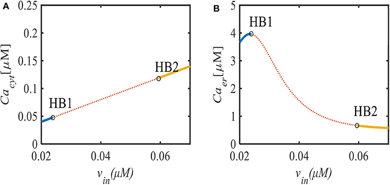
Figure 1. (A) Bifurcation diagram of the equilibrium of system (2) in the (v_in, Ca_cyt)-plane. (B) Bifurcation diagram of the equilibrium of system (2) in the (v_in, Ca_er)-plane. Points HB1 and HB2 are the Hopf bifurcation points.

In Figure 2, we shall present the time evolutions of cytosol Ca²⁺ concentration in this model for different values of the parameter v_in by numerical simulation. The left panels represent time series of Ca_cyt comparison of parameter v_in, and the right panels are the corresponding Ca_cyt-Ca_er-IP₃ phase portrait. For example, there is a single peak in this type of oscillation for v_in = 0.024 μM/s in Figure 2A, and the corresponding 3D phase-space is shown in Figure 2B. Around v_in = 0.033 μM/s, it is seen that the number of peak counts and peak magnitude begin to increase, as shown in Figures 2C,D. Similarly, when v_in = 0.052 μM/s, five peaks were obtained (Figures 2E,F). Moreover, it should be mentioned in Figures 2G,E, although the results for peak magnitude look very similar and in agreement with the peak counts, that the oscillatory vibration is significantly different (Figures 2G,H).

FIGURE 2

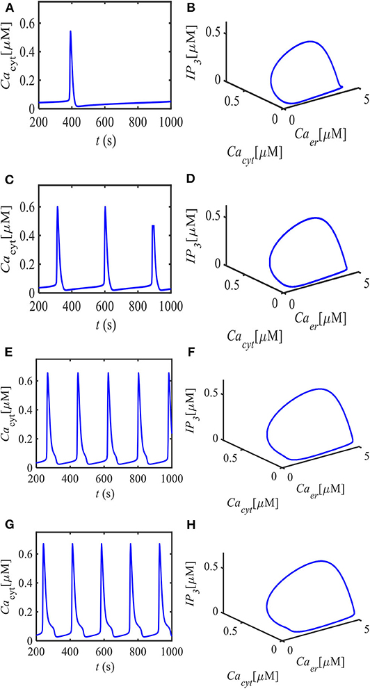
Figure 2. Spontaneous Ca²⁺ oscillations in astrocytes emerged at different parts of the curve in Figure 1 relative to points HB1 and HB2. The left panels denote the time evolution of Ca_cyt for different sets of parameter v_in, and the right panels denote the corresponding Ca_cyt-Ca_er-IP₃ phase portrait. (A) v_in = 0.024 μM/s, (B) portrait diagram as v_in = 0.024 μM/s, (C) v_in = 0.033 μM/s, (D) portrait diagram as v_in = 0.033 μM/s, (E) v_in = 0.052 μM/s, (F) portrait diagram as v_in = 0.052 μM/s, (G) v_in = 0.0593 μM/s, and (H) portrait diagram as v_in = 0.0593 μM/s.

Conclusion

In this paper, we have theoretically investigated the stability of equilibrium and bifurcation of spontaneous Ca²⁺ oscillations with a mathematical model in astrocytes. By choosing the flow of Ca²⁺ from the extracellular vesicles through the membrane and into the cytosol as the bifurcation parameter, we conclude that two subcritical Hopf bifurcation points play an important role in the occurrence of Ca²⁺ oscillations. By combining the theoretical analysis results in this paper, we numerically gave the Hopf bifurcations, which agree with the theoretical results. Our results may be instructive for better understanding the role of spontaneous Ca²⁺ oscillations in astrocytes. Because synchronization of different oscillatory patterns may relate to bifurcation, we will give detailed research in future.

Data Availability Statement

All datasets generated for this study are included in the article/supplementary material.

Author Contributions

HZ and MY contributed to the conception and design of the study. HZ organized the literature and wrote the first draft of the manuscript. MY performed the design of figures. All authors contributed to the manuscript revision and read and approved the submitted version.

Funding

This work was supported by the Natural Science Foundation of China under Grant No. 11872084 and the Natural Science Foundation of the Anhui Higher Education Institutions of China under Grant Nos. KJ2016SD54 and KJ2017A460.

Conflict of Interest

The authors declare that the research was conducted in the absence of any commercial or financial relationships that could be construed as a potential conflict of interest.

References

1. Scemes E, Giaume C. Astrocyte calcium waves: what they are and what they do. Glia. (2006) 54:716–25. doi: 10.1002/glia.20374

PubMed Abstract | CrossRef Full Text | Google Scholar

2. Nedergaard M, Ransom B, Goldman SA. New roles for astrocytes: redefining the functional architecture of the brain. Trends Neurosci. (2003) 26:523–30. doi: 10.1016/j.tins.2003.08.008

PubMed Abstract | CrossRef Full Text | Google Scholar

3. Agulhon C, Petravicz J, McMullen AB, Sweger EJ, Minton SK, Taves SR, et al. What is the role of astrocyte calcium in neurophysiology? Neuron. (2008) 59:932–46. doi: 10.1016/j.neuron.2008.09.004

PubMed Abstract | CrossRef Full Text | Google Scholar

4. Anwar H. Capturing intracellular Ca²⁺ dynamics in computational models of neurodegenerative diseases. Drug Discov Today Dis Models. (2016) 19:37–42. doi: 10.1016/j.ddmod.2017.02.005

PubMed Abstract | CrossRef Full Text | Google Scholar

5. Toth AB, Hori K, Novakovic MM, Bernstein NG, Lambot L, Prakriya M. CRAC channels regulate astrocyte Ca²⁺ signaling and gliotransmitter release to modulate hippocampal GABAergic transmission. Sci Signal. (2019) 12:eaaw5450. doi: 10.1126/scisignal.aaw5450

PubMed Abstract | CrossRef Full Text | Google Scholar

6. Volterra A, Meldolesi J. Astrocytes, from brain glue to communication elements: the revolution continues. Nat Rev Neurosci. (2005) 6:626–40. doi: 10.1038/nrn1722

PubMed Abstract | CrossRef Full Text | Google Scholar

7. Halnes G, Østby I, Pettersen KH, Omholt SW, Einevoll GT. Electrodiffusive model for astrocytic and neuronal ion concentration dynamics. PLoS Comput Biol. (2013) 9:e1003386. doi: 10.1371/journal.pcbi.1003386

PubMed Abstract | CrossRef Full Text | Google Scholar

8. Charles AC. Glia-neuron intercellular calcium signaling. Dev Neurosci. (1994) 16:196–206. doi: 10.1159/000112107

PubMed Abstract | CrossRef Full Text | Google Scholar

9. Matrosov VV, Kazantsev VB. Bifurcation mechanisms of regular and chaotic network signaling in brain astrocytes. Chaos. (2011) 21:023103. doi: 10.1063/1.3574031

PubMed Abstract | CrossRef Full Text | Google Scholar

10. Ji Q, Lu Y. Bifurcations and continuous transitions in a nonlinear model of intracellular calcium oscillations. Int J Bifurcat Chaos. (2013) 23:1350033. doi: 10.1142/S0218127413500338

CrossRef Full Text | Google Scholar

11. Liu H, Pan Y, and Cao J. Composite learning adaptive dynamic surface control of fractional-order nonlinear systems. IEEE Trans Syst Man Cybernetics. (2019) 50:2557–67. doi: 10.1109/tcyb.2019.2938754

PubMed Abstract | CrossRef Full Text | Google Scholar

12. Liu H, Wang H, Cao J, Alsaedi A, Hayat T. Composite learning adaptive sliding mode control of fractional-order nonlinear systems with actuator faults. J Franklin Inst. (2019) 36:9580–99. doi: 10.1016/j.franklin.2019.02.042

CrossRef Full Text | Google Scholar

13. Parri HR, Gould TM, Crunelli V. Spontaneous astrocytic Ca 2+ oscillations in situ drive NMDAR-mediated neuronal excitation. Nat Neurosci. (2001) 4:803–12. doi: 10.1038/90507

PubMed Abstract | CrossRef Full Text | Google Scholar

14. Ding X, Zhang X, Ji L. Contribution of calcium fluxes to astrocyte spontaneous calcium oscillations in deterministic and stochastic models. Appl Math Model. (2018) 55:371–82. doi: 10.1016/j.apm.2017.11.002

CrossRef Full Text | Google Scholar

15. Li J, Tang J, Ma J, Du M, Wang R, Wu Y. Dynamic transition of neuronal firing induced by abnormal astrocytic glutamate oscillation. Sci Rep. (2016) 6:32343. doi: 10.1038/srep32343

PubMed Abstract | CrossRef Full Text | Google Scholar

16. Ji Q, Zhou Y, Yang Z, Meng X. Evaluation of bifurcation phenomena in a modified Shen–Larter model for intracellular Ca²⁺ bursting oscillations. Nonlinear Dyn. (2016) 84:1281–8. doi: 10.1007/s11071-015-2566-3

CrossRef Full Text | Google Scholar

17. Oschmann F, Berry H, Obermayer K, Lenk K. From in silico astrocyte cell models to neuron-astrocyte network models: a review. Brain Res Bull. (2018) 136:76–84. doi: 10.1016/j.brainresbull.2017.01.027

PubMed Abstract | CrossRef Full Text | Google Scholar

18. Matrosov V, Gordleeva S, Boldyreva N, Ben-Jacob E, Kazantsev V, de Pitta M, et al. Emergence of regular and complex calcium oscillations by inositol 1,4,5-Trisphosphate signaling in astrocytes. Neurons Cogn. (2019) 151–76. doi: 10.1007/978-3-030-00817-8_6

CrossRef Full Text | Google Scholar

19. Zhou A, Liu X, Yu P. Bifurcation analysis on the effect of store-operated and receptor-operated calcium channels for calcium oscillations in astrocytes. Nonlinear Dyn. (2019) 97:1–16. doi: 10.1007/s11071-019-05009-2

CrossRef Full Text | Google Scholar

20. Engelborghs K, Luzyanina T, Roose D. Numerical bifurcation analysis of delay differential equations using DDE-BIFTOOL. ACM Trans Math Softw. (2002) 28:1–21. doi: 10.1145/513001.513002

CrossRef Full Text | Google Scholar

21. Yu P, Leung AY. The simplest normal form of Hopf bifurcation. Nonlinearity. (2003) 16:277–300. doi: 10.1088/0951-7715/16/1/317

CrossRef Full Text | Google Scholar

22. Yuan Y, Belair J. Stability and hopf bifurcation analysis for functional differential equation with distributed delay. Siam J Appl Dyn Syst. (2011) 10:551–81. doi: 10.1137/100794493

CrossRef Full Text | Google Scholar

23. Kopell N, Ermentrout GB, Whittington MA, Traub RD. Gamma rhythms and beta rhythms have different synchronization properties. Proc Natl Acad Sci USA. (2000) 97:1867–72. doi: 10.1073/pnas.97.4.1867

PubMed Abstract | CrossRef Full Text | Google Scholar