Dynamic investigation of the Laksmanan–Porsezian–Daniel model with Kerr, parabolic, and anti-cubic laws of nonlinearities

1 Introduction

The world is not as simple as it seems. Every mechanism around the world contains many changing factors and nonlinearities. Nonlinear partial differential equations (NPDEs) provide best mathematical tools for modeling of such mechanisms. Many nonlinear physical phenomena are modeled by NPDEs in physics, fluid dynamics, mathematical biology, and optical fibers. Some NPDEs such as Navier–Stokes equations [1], shallow water-like equations [2], Witham equation [3], complex coupled Higgs model [4], and nonlinear Schrödinger equation [5] are used to represent different natural phenomena and dynamical processes.The breaking of nonlinear dispersive water wave phenomena is modeled by Witham equations. Navier–Stokes equations and shallow water-like equations are utilized for modeling of water waves, atmospheric flow, and many other fluid dynamics. In quantum mechanics, optics, and fluid dynamics, the Schrödinger equation is used to represent many dynamical processes and wave phenomena.The nonlinear Schrödinger equation is one of the most significant evolution equations arising in nonlinear optics. It is used to describe the propagation of light pulses through optical fibers. The study of optical solitons is essential to understand and improve the data transmission through optical fibers over long intervals. Optical solitons are electromagnetic solitary waves that arise due to the balance of nonlinear and dispersive effects and allow carry data over long distances. The optical soliton theory is used in many applications of telecommunications, ocean engineering, and other areas of science [6–8].The nonlinear Schrödinger equation and its different modified forms have been explored by many researchers to understand the light propagation through optical media. Some recent studies have reported useful results on the optical soliton theory using the ansatz method [9], Jacobi elliptic method [10], extended tanh–coth expansion technique [11], and Kudryashov expansion technique [12].

This paper deals with the Lakshmanan–Porsezian–Daniel (LPD) model, which first appeared in 1988 [13]. The LPD model is an important type of the Schrödinger equation and widely studied in optical fibers, physics, and engineering [14]. The LPD model is one of the significant evolution equations used in physics and other science fields. During the past few years, the LPD model has been investigated using different techniques such as the modified simple equation method [15], modified auxiliary equation method [16,17], extended trial equation technique [18], modified extended direct algebraic technique [19], improved Adomian decomposition technique [20], and generalized projective Riccati equation technique [21].In this study, the optical solitons of the LPD model are retrieved using the extended $\left(\frac{G^{\prime }}{G^2}\right)$-expansion technique along with other traveling wave solutions. The LPD model is a useful model for the description of nonlinear waves through optical media in many real-life problems [15]. The LPD model of the following form is considered:

$i{\mathrm{\Lambda }}_t+a{\mathrm{\Lambda }}_{xx}+b{\mathrm{\Lambda }}_{xt}+\tau F\left(|\mathrm{\Lambda }{|}^2\right)\mathrm{\Lambda }=\sigma {\mathrm{\Lambda }}_{\mathit{x}\mathit{x}\mathit{x}\mathit{x}}+\gamma {\left({\mathrm{\Lambda }}_x\right)}^2{\mathrm{\Lambda }}^{*}+\beta |{\mathrm{\Lambda }}_x{|}^2\mathrm{\Lambda }+\mu |\mathrm{\Lambda }{|}^2{\mathrm{\Lambda }}_{xx}+\varrho {\mathrm{\Lambda }}^2{\mathrm{\Lambda }}_{xx}^{*}+ϵ|\mathrm{\Lambda }{|}^4\mathrm{\Lambda },(1)$

where Λ(x, t) represents the wave profile. In the LPD model, dispersion is of higher order, fully nonlinear, and spatio-temporal in nature. On the left hand side of Eq. 1, the first term depicts the temporal evolution, the coefficient a is the GVD, and b is the spatio-temporal dispersal. The nonlinear functional F is a real-valued algebraic function F (|Λ|²)Λ: C → C which ensures the continuity of the LPD model. Moreover,

$F\left(|\mathrm{\Lambda }{|}^2\right)\mathrm{\Lambda }\in \bigcup _{m,n=1}^{\infty }{C}^k\left(\left(-m,m\right)\times \left(-n,n\right);R^2\right),(2)$

where the complex plane C is treated as the two-dimensional linear space R². A fourth-order dispersion coefficient σ is on the right side of Eq. 1, whereas a two-photon absorption coefficient ϵ is in the last term of the right side. The coefficients γ, γ₁, μ, and λ indicate perturbation terms with nonlinear forms of dispersion.In recent decades, the study of exact soliton solutions for NPDEs has become a vital topic in many nonlinear science fields. Many nonlinear physical phenomena can be understood by analyzing the exact solutions to NPDEs. To obtain the exact solutions to NPDEs, many researchers developed different exact methods. Many exact methods, for e.g., the extended $\left(\frac{G^{\prime }}{G^2}\right)$-expansion method [22], extended sine–cosine method [23], and modified Kudryashov method [24], are utilized to acquire the exact soliton solutions to NPDEs.The aim of this research paper is to obtain closed form soliton solutions of the LPD model using the extended $\left(\frac{G^{\prime }}{G^2}\right)$-expansion method. The proposed exact technique provides a variety of soliton solutions of a wide range of nonlinear evolution equations [25]. It is an efficient, reliable, and straight-forward technique to explore nonlinear models. The following section describes the algorithm of the proposed method.

2 Description of the extended $(\frac{G^{\prime }}{G^2})$-expansion method

Description of the method is given as follows:

Step 1: NPDE of the following form is considered:

$Q\left(P,P_x,P_t,P_{xx},P_{xt},P_{tt}\dots \right)=0,(3)$

where Eq. 3 represents the function P (x, t) and its partial derivatives.

Step 2: The following travailing wave transformations are applied to transform Eq. 3 into ODE:

$P\left(x,t\right)=\mathrm{\Gamma }\left(\zeta \right),\zeta =\kappa x\pm ct,(4)$

Using Eq. 4, ODE of the following form is obtained:

$T\left(\mathrm{\Gamma },{\mathrm{\Gamma }}^{\prime },{\mathrm{\Gamma }}^{″},\dots \right)=0,(5)$

where k and c are constants and ${\mathrm{\Gamma }}^{\prime }=\frac{d\mathrm{\Gamma }}{d\zeta }$.

Step 3: According to the proposed exact method, a formal solution to Eq. 5 is considered as follows:

$\mathrm{\Gamma }\left(\zeta \right)=a_0+\sum _{j=1}^{j=M}\left[a_j{\left(\frac{G^{\prime }}{G^2}\right)}^j+b_j{\left(\frac{G^{\prime }}{G^2}\right)}^{-j}\right].(6)$

The first derivative of the function G = G(ζ) is expressed as

${\left(\frac{G^{\prime }}{G^2}\right)}^{\prime }={\vartheta }_1+{\vartheta }_2{\left(\frac{G^{\prime }}{G^2}\right)}^2.(7)$

In Eqs 6, 7, a₀, a_j, and b_j are unknown parametric values to be extracted with ϑ₁ ≠ 1 and ϑ₂ ≠ 0.

Step 4: The highest order derivative’s degree and nonlinear term’s degree can be balanced to extract the value of M by utilizing the homogeneous balance principle (HBP), which is given as

$\mathit{deg}\left(\frac{d^N\mathrm{\Gamma }\left(\zeta \right)}{d{\zeta }^N}\right)=M+N,(8)$

$\mathit{deg}\left({\left(\mathrm{\Gamma }\left(\zeta \right)\right)}^L{\left(\frac{d^N\mathrm{\Gamma }\left(\zeta \right)}{d{\zeta }^N}\right)}^s\right)=ML+s\left(M+N\right).(9)$

Step 5: Eq. 6 with Eq. 7 will be applied in Eq. 5, and the coefficients of ${(\frac{G^{\prime }}{G^2})}^i,(i=0,\pm 1,\pm 2,\dots )$ will be equated to zero. The system of linear algebraic equations is obtained. This system is solved using an analytic tool, Maple software.

Step 6: The following three cases address the solution of Eq. 7.If ϑ₁ϑ₂ > 0, then the solution is given as

$\frac{G^{\prime }}{G^2}=\sqrt{\frac{{\vartheta }_1}{{\vartheta }_2}}\left(\frac{C\cos \sqrt{{\vartheta }_1{\vartheta }_2}\zeta +D\sin \sqrt{{\vartheta }_1{\vartheta }_2}\zeta }{D\cos \sqrt{{\vartheta }_1{\vartheta }_2}\zeta -C\sin \sqrt{{\vartheta }_1{\vartheta }_2}\zeta }\right).(10)$

If ϑ₁ϑ₂ < 0, then the solution is given as

$\frac{G^{\prime }}{G^2}=\frac{1}{2{\vartheta }_2}\left(2\sqrt{|{\vartheta }_1{\vartheta }_2|}-\frac{4C\sqrt{|{\vartheta }_1{\vartheta }_2|}{e}^{2\zeta \sqrt{|{\vartheta }_1{\vartheta }_2|}}}{C{e}^{2\zeta \sqrt{|{\vartheta }_1{\vartheta }_2|}}-D}\right).(11)$

If ϑ₁ = 0 and ϑ₂ ≠ 0, then the solution is given as

$\frac{G^{\prime }}{G^2}=-\frac{C}{{\vartheta }_2\left(C\zeta +D\right)},(12)$

where C, D are any real valued nonzero constants.

3 Application of the proposed method

This section includes the application of the proposed method to extract the exact soliton solutions of the LPD model. The following transformations are utilized:

$\begin{array}{ll}\hfill \mathrm{\Lambda }\left(x,t\right)& =\mathrm{\Lambda }\left(\zeta \right)e^{i\mathrm{\Theta }\left(x,t\right)},{\mathrm{\Lambda }}^{*}\left(x,t\right)=\mathrm{\Lambda }\left(\zeta \right)e^{-i\mathrm{\Theta }\left(x,t\right)},\hfill \\ \hfill \zeta & =x-ct,\mathrm{\Theta }\left(x,t\right)=-\kappa x+\omega t+\theta ,\hfill \end{array}(13)$

to transform Eq. 1 in ODE, which is given as

$\begin{array}{ll}\hfill & \sigma {\mathrm{\Gamma }}^{⁗}+\left(bv-6{\kappa }^2\sigma -a\right){\mathrm{\Gamma }}^{″}+\left({\kappa }^4\sigma -b\kappa \omega +a{\kappa }^2+\omega \right)\mathrm{\Gamma }-{\kappa }^2{\mathrm{\Gamma }}^3\left({\gamma }_1-{\vartheta }_2-\mu -\gamma \right)+ϵ{\mathrm{\Gamma }}^5\hfill \\ \hfill & -\tau F\left({\mathrm{\Gamma }}^2\right)\mathrm{\Gamma }+\left(\gamma +{\gamma }_1\right)\mathrm{\Gamma }{\left({\mathrm{\Gamma }}^{\prime }\right)}^2+\left({\vartheta }_2+\mu \right){\mathrm{\Gamma }}^2{\mathrm{\Gamma }}^{″}+\left(\left(-v+b\omega -4{\kappa }^3\sigma -2a\kappa +b\kappa v\right){\mathrm{\Gamma }}^{\prime }\right.\hfill \\ \hfill & \left.+2\left(\mu +\gamma -{\vartheta }_2\right)\kappa {\mathrm{\Gamma }}^2{\mathrm{\Gamma }}^{\prime }+4\kappa \sigma \mathrm{\Gamma }‴\right)i=0.\hfill \end{array}(14)$

In Eq. 14, κ, θ, ω, and c are the constants to be evaluated.Eq. 13 includes real and imaginary parts. Taking the real part of the equation equal to zero, the following relation is determined:

$\begin{array}{ll}\hfill & \sigma {\mathrm{\Gamma }}^{⁗}+\left(bv-6{\kappa }^2\sigma -a\right){\mathrm{\Gamma }}^{″}+\left({\kappa }^4\sigma -b\kappa \omega +a{\kappa }^2+\omega \right)\mathrm{\Gamma }-{\kappa }^2\left(\varrho -{\gamma }_1+\mu +\gamma \right){\mathrm{\Gamma }}^3+ϵ{\mathrm{\Gamma }}^5-\tau F\left({\mathrm{\Gamma }}^2\right)\mathrm{\Gamma }+\left(\gamma +{\gamma }_1\right)\mathrm{\Gamma }{\left({\mathrm{\Gamma }}^{\prime }\right)}^2+\left(\varrho +\mu \right){\mathrm{\Gamma }}^2{\mathrm{\Gamma }}^{″}=0,\hfill \end{array}(15)$

while the imaginary part of the equation is derived as

$\left(b\kappa v+b\omega -4{\kappa }^3\sigma -v-2a\kappa \right){\mathrm{\Gamma }}^{\prime }+2\kappa \left(\mu +\gamma -{\vartheta }_2\right){\mathrm{\Gamma }}^2{\mathrm{\Gamma }}^{\prime }+4\kappa \sigma \mathrm{\Gamma }‴=0.(16)$

The coefficients of the linearly independent functions are considered zero in Eqs 14, 15. Consequently, the following constraints are obtained:

$\gamma +{\gamma }_1=0,(17)$

$\varrho +\mu =0,(18)$

$\sigma =0,(19)$

$\gamma +\mu -\varrho =0,(20)$

$v=\frac{2a\kappa -b\omega }{b\kappa -1},b\kappa -1\ne 0.(21)$

In Eq. 21, v depicts the speed of the wave. By substituting Eqs 17–21, Eqs 14, 16 reduce to a single equation as

$\left(-bv+a\right){\mathrm{\Gamma }}^{″}+\left(b\kappa \omega -\omega -a{\kappa }^2\right)\mathrm{\Gamma }-4\mu {\kappa }^2{\mathrm{\Gamma }}^3-ϵ{\mathrm{\Gamma }}^5+\tau F\left(|\mathrm{\Gamma }{|}^2\right)\mathrm{\Gamma }=0.(22)$

The following subsection includes the extraction of soliton solutions of the proposed equation involving the Kerr law of nonlinearity.

3.1 Kerr law

The Kerr law of nonlinearity implies

$F\left(|\mathrm{\Lambda }{|}^2\right)=|\mathrm{\Lambda }{|}^2.(23)$

Eq. 1 is transformed into the following form:

$i{\mathrm{\Lambda }}_t+a{\mathrm{\Lambda }}_{xx}+b{\mathrm{\Lambda }}_{xt}+\tau |\mathrm{\Lambda }{|}^2\mathrm{\Lambda }=-2\mu {\left({\mathrm{\Lambda }}_x\right)}^2{\mathrm{\Lambda }}^{*}+2\mu |{\mathrm{\Lambda }}_x|\mathrm{\Lambda }+\mu |\mathrm{\Lambda }{|}^2{\mathrm{\Lambda }}_{xx}-\mu {\mathrm{\Lambda }}^2{\mathrm{\Lambda }}_{xx}^{*}+ϵ|\mathrm{\Lambda }{|}^4\mathrm{\Lambda },(24)$

and Eq. 22 is simplified as

$\left(a-bv\right){\mathrm{\Gamma }}^{″}+\left(b\kappa \omega -a{\kappa }^2-\omega \right)\mathrm{\Gamma }+\left(\tau -4\mu {\kappa }^2\right){\mathrm{\Gamma }}^3-ϵ{\mathrm{\Gamma }}^5=0.(25)$

Using the transformation $\mathrm{\Gamma }={\mathrm{\Delta }}^{\frac{1}{2}}$, Eq. 25 becomes

$\left(a-b\mathrm{\Delta }\right)\left(-{\left({\mathrm{\Delta }}^{\prime }\right)}^2+2\mathrm{\Delta }{\mathrm{\Delta }}^{″}\right)+4\left(b\kappa \omega -a{\kappa }^2-\omega \right){\mathrm{\Delta }}^2+4\left(\tau -4\mu {\kappa }^2\right){\mathrm{\Delta }}^3-4ϵ{\mathrm{\Delta }}^4=0.(26)$

The degrees of the nonlinear term Δ⁴ and highest order derivative term ΔΔ′′ are balanced at M = 1 by utilizing HBP. The solution of Eq. 26 from Eq. 6 is written as

$\mathrm{\Delta }=a_0+a_1\left(\frac{G^{\prime }}{G^2}\right)+b_1{\left(\frac{G^{\prime }}{G^2}\right)}^{-1}.(27)$

In Eq. 27, a₀, a₁, and b₁ are the constants to be evaluated. Eq. 27 with Eq. 7 is substituted into Eq. 26, and the coefficients of ${\left(\frac{G^{\prime }}{G^2}\right)}^i$ are accumulated, where (i = 0, ±1, ±2, … ). These coefficients are set equal to zero, and as a result, a system of linear algebraic equations is acquired. This system of linear equations is solved simultaneously. As a result, the following sets of solutions are obtained:Set 1

$\begin{array}{ll}\hfill \kappa & =\pm \frac{\sqrt{3\tau \mu +2aϵ\mp 2\sqrt{a^2{ϵ}^2+3a\tau ϵ\mu }}}{2\sqrt{3}\mu },\hfill \\ \hfill b_1& =\pm \sqrt{-\frac{a{\vartheta }_1\left(2aϵ+3\tau \mu \mp 2\sqrt{aϵ\left(aϵ+3\tau \mu \right)}\right)}{2ϵ{\vartheta }_2{\mu }^2}},\omega =0,\hfill \\ \hfill v& =\frac{a\left(12{\vartheta }_2{\vartheta }_1{\mu }^2+3\tau \mu +2aϵ\pm 2\sqrt{aϵ\left(aϵ+3\tau \mu \right)}\right)}{12{\mu }^2{\vartheta }_1{\vartheta }_{2}b},\hfill \\ \hfill a_0& =\pm \frac{aϵ\pm \sqrt{aϵ\left(aϵ+3\tau \mu \right)}}{4\mu ϵ},a_1=0.\hfill \end{array}$

Set 2

$\begin{array}{ll}\hfill \omega & =-\frac{48{\mu }^2{\kappa }^4-16aϵ{\kappa }^2-24\tau \mu {\kappa }^2+3{\tau }^2}{16ϵ\left(b\kappa -1\right)},v=\frac{48{\mu }^2{\kappa }^4+16aϵ{\vartheta }_2{\vartheta }_1-24\tau \mu {\kappa }^2+3{\tau }^2}{16{\vartheta }_2{\vartheta }_1ϵb},\kappa =\kappa ,\hfill \\ a_0=-\frac{3}{8}\frac{4\mu {\kappa }^2-\tau }{ϵ},a_1=\pm \frac{3}{8}\frac{\sqrt{-\frac{{\vartheta }_2}{{\vartheta }_1}}\left(4\mu {\kappa }^2-\tau \right)}{ϵ},b_1=0.\hfill \end{array}$

Set 3

$\kappa =\frac{1}{2}\frac{\sqrt{\tau }}{\sqrt{\mu }},\omega =0,v=\frac{1}{4}\frac{a\left(4\mu {\vartheta }_2{\vartheta }_1+\tau \right)}{{\vartheta }_2\mu {\vartheta }_{1}b},a_0=0,a_1=\pm \sqrt{-\frac{3}{16}\frac{a\tau {\vartheta }_2}{ϵ\mu {\vartheta }_1}},b_1=\pm \frac{1}{4}\frac{a\tau \sqrt{3}}{ϵ\sqrt{-\frac{a\tau \mu {\vartheta }_2}{ϵ{\vartheta }_1}}}.$

Set 4

$\begin{array}{ll}\hfill \kappa & =\pm \frac{\sqrt{3}\sqrt{3\tau \mu +2aϵ\pm 2\sqrt{a^2{ϵ}^2+3a\tau ϵ\mu }}}{6\mu },\hfill \\ \hfill v& =\frac{a\left(12{\vartheta }_2{\vartheta }_1{\mu }^2+3\tau \mu +2aϵ\pm \sqrt{aϵ\left(aϵ+3\tau \mu \right)}\right)}{12{\mu }^2{\vartheta }_1{\vartheta }_{2}b},\hfill \\ \hfill a_0& =\pm \frac{aϵ\pm \sqrt{aϵ\left(aϵ+3\tau \mu \right)}}{4\mu ϵ},\hfill \\ \hfill a_1& =\pm \sqrt{-\frac{3\mu a\tau {\vartheta }_2+2a^2ϵ{\vartheta }_2\pm 2a{\vartheta }_2\sqrt{a^2{ϵ}^2+3a\tau ϵ\mu }}{16{\mu }^2ϵ{\vartheta }_1}},b_1=0,\omega =0.\hfill \end{array}$

Set 5

$\begin{array}{ll}\hfill \kappa & =\pm \frac{\sqrt{13}\sqrt{15\tau \mu +8aϵ\pm 4\sqrt{4a^2{ϵ}^2+15a\tau ϵ\mu }}}{30\mu },\omega =0,\hfill \\ \hfill a_0& =-\frac{2aϵ\pm \sqrt{aϵ\left(4aϵ+15\tau \mu \right)}}{10\mu ϵ},\hfill \\ \hfill a_1& =\pm \sqrt{-\frac{-15\mu a\tau {\vartheta }_2-8a^2ϵ{\vartheta }_2\mp 4\sqrt{4a^2{ϵ}^2+15a\tau ϵ\mu a{\vartheta }_2}}{400{\mu }^2ϵ{\vartheta }_1}},\hfill \\ \hfill b_1& =\pm \frac{a\left(8aϵ+15\tau \mu \mp 4\sqrt{aϵ\left(4aϵ+15\tau \mu \right)}\right)}{20\sqrt{\frac{a{\vartheta }_2\left(8aϵ+15\tau \mu +4\sqrt{aϵ\left(4aϵ+15\tau \mu \right)}\right)}{ϵ{\vartheta }_1}\mu ϵ}}.\hfill \end{array}$

By utilizing values from sets 1 to 5, following families of solutions of Eq. 1 are obtained.

Family 1

This family of solutions is obtained by taking values from Set 1.

$\mathrm{\Lambda }\left(x,t\right)={\left(\pm \frac{1}{4}\frac{aϵ\pm \sqrt{aϵ\left(aϵ+3\tau \mu \right)}}{\mu ϵ}\pm \frac{1}{4}\sqrt{-\frac{a{\vartheta }_1\left(2aϵ+3\tau \mu \mp 2\sqrt{aϵ\left(aϵ+3\tau \mu \right)}\right)}{ϵ{\vartheta }_2{\mu }^2}}{\left(\frac{G^{\prime }}{G^2}\right)}^{-1}\right)}^{\frac{1}{2}}{e}^{i\mathrm{\Theta }}.(28)$

For ϑ₁ϑ₂ > 0,

$\begin{array}{ll}\hfill {\mathrm{\Lambda }}_1^1\left(x,t\right)& =\left(\pm \frac{1}{4}\frac{aϵ\pm \sqrt{aϵ\left(aϵ+3\tau \mu \right)}}{\mu ϵ}\pm \frac{1}{4}\sqrt{-\frac{a{\vartheta }_1\left(2aϵ+3\tau \mu \mp 2\sqrt{aϵ\left(aϵ+3\tau \mu \right)}\right)}{ϵ{\vartheta }_2{\mu }^2}}\right.\hfill \\ \hfill & {\left.\times {\left(\sqrt{\frac{{\vartheta }_1}{{\vartheta }_2}}\left(\frac{C\cos \sqrt{{\vartheta }_1{\vartheta }_2}\zeta +D\sin \sqrt{{\vartheta }_1{\vartheta }_2}\zeta }{D\cos \sqrt{{\vartheta }_1{\vartheta }_2}\zeta -C\sin \sqrt{{\vartheta }_1{\vartheta }_2}\zeta }\right)\right)}^{-1}\right)}^{\frac{1}{2}}{e}^{i\mathrm{\Theta }}.\hfill \end{array}(29)$

For ϑ₁ϑ₂ < 0,

$\begin{array}{ll}\hfill {\mathrm{\Lambda }}_2^1\left(x,t\right)& =\left(\pm \frac{1}{4}\frac{aϵ\pm \sqrt{aϵ\left(aϵ+3\tau \mu \right)}}{\mu ϵ}\pm \frac{1}{4}\sqrt{-\frac{a{\vartheta }_1\left(2aϵ+3\tau \mu \mp 2\sqrt{aϵ\left(aϵ+3\tau \mu \right)}\right)}{ϵ{\vartheta }_2{\mu }^2}}\right.\hfill \\ \hfill & \times {\left(\frac{1}{2{\vartheta }_2}{\left(2\sqrt{|{\vartheta }_1{\vartheta }_2|}-\frac{4C\sqrt{|}{\vartheta }_1{\vartheta }_2|e^{2\zeta \sqrt{|{\vartheta }_1{\vartheta }_2|}}}{C{e}^{2\zeta \sqrt{|{\vartheta }_1{\vartheta }_2|}}-D}\right)}^{-1}\right)}^{\frac{1}{2}}{e}^{i\mathrm{\Theta }}.\hfill \end{array}(30)$

For ϑ₁ = 0 and ϑ₂ ≠ 0,

$\begin{array}{ll}\hfill {\mathrm{\Lambda }}_3^1\left(x,t\right)& =\left(\pm \frac{1}{4}\frac{aϵ\pm \sqrt{aϵ\left(aϵ+3\tau \mu \right)}}{\mu ϵ}\pm \frac{1}{4}\sqrt{-\frac{a{\vartheta }_1\left(2aϵ+3\tau \mu \mp 2\sqrt{aϵ\left(aϵ+3\tau \mu \right)}\right)}{ϵ{\vartheta }_2{\mu }^2}}\right.\hfill \\ \hfill & \times {\left.{\left(-\frac{C}{{\vartheta }_2\left(C\zeta +D\right)}\right)}^{-1}\right)}^{\frac{1}{2}}{e}^{i\mathrm{\Theta }}.\hfill \end{array}(31)$

Family 2

This family of solutions is obtained by taking values from Set 2.

$\mathrm{\Lambda }\left(x,t\right)={\left(-\frac{3}{8}\frac{4\mu {\kappa }^2-\tau }{ϵ}\pm \frac{3}{8}\frac{\sqrt{-\frac{{\vartheta }_2}{{\vartheta }_1}}\left(4\mu {\kappa }^2-\tau \right)}{ϵ}\left(\frac{G^{\prime }}{G^2}\right)\right)}^{\frac{1}{2}}{e}^{i\mathrm{\Theta }}.(32)$

For ϑ₁ϑ₂ > 0,

$\begin{array}{ll}\hfill {\mathrm{\Lambda }}_1^2\left(x,t\right)& =\left(-\frac{3}{8}\frac{4\mu {\kappa }^2-\tau }{ϵ}\right.\hfill \\ \hfill & {\left.\pm \frac{3}{8}\frac{\sqrt{-\frac{{\vartheta }_2}{{\vartheta }_1}}\left(4\mu {\kappa }^2-\tau \right)}{ϵ}\sqrt{\frac{{\vartheta }_1}{{\vartheta }_2}}\left(\frac{C\cos \sqrt{{\vartheta }_1{\vartheta }_2}\zeta +D\sin \sqrt{{\vartheta }_1{\vartheta }_2}\zeta }{D\cos \sqrt{{\vartheta }_1{\vartheta }_2}\zeta -C\sin \sqrt{{\vartheta }_1{\vartheta }_2}\zeta }\right)\right)}^{\frac{1}{2}}{e}^{i\mathrm{\Theta }}.\hfill \end{array}(33)$

For ϑ₁ϑ₂ < 0,

$\begin{array}{ll}\hfill {\mathrm{\Lambda }}_2^2\left(x,t\right)& =\left(-\frac{3}{8}\frac{4\mu {\kappa }^2-c}{ϵ}\right.\hfill \\ \hfill & \pm \frac{3}{8}\frac{\sqrt{-\frac{{\vartheta }_2}{{\vartheta }_1}}\left(4\mu {\kappa }^2-c\right)}{ϵ}{\left(\frac{1}{2{\vartheta }_2}\left(2\sqrt{|{\vartheta }_1{\vartheta }_2|}-\frac{4C\sqrt{|}{\vartheta }_1{\vartheta }_2|e^{2\zeta \sqrt{|{\vartheta }_1{\vartheta }_2|}}}{C{e}^{2\zeta \sqrt{|{\vartheta }_1{\vartheta }_2|}}-D}\right)\right)}^{\frac{1}{2}}{e}^{i\mathrm{\Theta }}.\hfill \end{array}(34)$

For ϑ₁ = 0 and ϑ₂ ≠ 0,

${\mathrm{\Lambda }}_3^2\left(x,t\right)={\left(-\frac{3}{8}\frac{4\mu {\kappa }^2-\tau }{ϵ}\pm \frac{3}{8}\frac{\sqrt{-\frac{{\vartheta }_2}{{\vartheta }_1}}\left(4\mu {\kappa }^2-\tau \right)}{ϵ}\left(-\frac{C}{{\vartheta }_2\left(C\zeta +D\right)}\right)\right)}^{\frac{1}{2}}{e}^{i\mathrm{\Theta }}.(35)$

Family 3

This family of solutions is obtained by taking values from Set 3.

$\mathrm{\Lambda }\left(x,t\right)={\left(\pm \sqrt{-\frac{3}{16}\frac{a\tau {\vartheta }_2}{ϵ\mu {\vartheta }_1}}\left(\frac{G^{\prime }}{G^2}\right)\pm \frac{1}{4}\frac{ac\sqrt{3}}{ϵ\sqrt{\mu }\sqrt{-\frac{a\tau {\vartheta }_2}{ϵ{\vartheta }_1}}}\sqrt{\frac{{\vartheta }_2}{{\vartheta }_1}}{\left(\frac{G^{\prime }}{G^2}\right)}^{-1}\right)}^{\frac{1}{2}}{e}^{i\mathrm{\Theta }}.(36)$

For ϑ₁ϑ₂ > 0,

$\begin{array}{ll}\hfill {\mathrm{\Lambda }}_1^3\left(x,t\right)& =\left(\pm \sqrt{-\frac{3}{16}\frac{a\tau {\vartheta }_2}{ϵ\mu {\vartheta }_1}}\left(\sqrt{\frac{{\vartheta }_1}{{\vartheta }_2}}\left(\frac{C\cos \sqrt{{\vartheta }_1{\vartheta }_2}\zeta +D\sin \sqrt{{\vartheta }_1{\vartheta }_2}\zeta }{D\cos \sqrt{{\vartheta }_1{\vartheta }_2}\zeta -C\sin \sqrt{{\vartheta }_1{\vartheta }_2}\zeta }\right)\right.\right.\hfill \\ \hfill & {\left.\pm \frac{1}{4}\frac{a\tau \sqrt{3}}{ϵ\sqrt{\mu }\sqrt{-\frac{a\tau {\vartheta }_2}{ϵ{\vartheta }_1}}}\sqrt{\frac{{\vartheta }_2}{{\vartheta }_1}}{\left(\frac{C\cos \sqrt{{\vartheta }_1{\vartheta }_2}\zeta +D\sin \sqrt{{\vartheta }_1{\vartheta }_2}\zeta }{D\cos \sqrt{{\vartheta }_1{\vartheta }_2}\zeta -C\sin \sqrt{{\vartheta }_1{\vartheta }_2}\zeta }\right)}^{-1}\right)}^{\frac{1}{2}}{e}^{i\mathrm{\Theta }}.\hfill \end{array}(37)$

For ϑ₁ϑ₂ < 0,

$\begin{array}{ll}\hfill {\mathrm{\Lambda }}_2^3\left(x,t\right)& =\left(\pm \sqrt{-\frac{3}{16}\frac{a\tau {\vartheta }_2}{ϵ\mu {\vartheta }_1}}\left(\frac{1}{2{\vartheta }_2}\left(2\sqrt{|{\vartheta }_1{\vartheta }_2|}-\frac{4C\sqrt{|}{\vartheta }_1{\vartheta }_2|e^{2\zeta \sqrt{|{\vartheta }_1{\vartheta }_2|}}}{C{e}^{2\zeta \sqrt{|{\vartheta }_1{\vartheta }_2|}}-D}\right)\right.\right.\hfill \\ \hfill & \pm \frac{1}{4}\frac{a\tau \sqrt{3}}{ϵ\sqrt{\mu }\sqrt{-\frac{a\tau {\vartheta }_2}{ϵ{\vartheta }_1}}}{\left(\frac{1}{2{\vartheta }_2}{\left(2\sqrt{|{\vartheta }_1{\vartheta }_2|}-\frac{4C\sqrt{|}{\vartheta }_1{\vartheta }_2|e^{2\zeta \sqrt{|{\vartheta }_1{\vartheta }_2|}}}{C{e}^{2\zeta \sqrt{|{\vartheta }_1{\vartheta }_2|}}-D}\right)}^{-1}\right)}^{\frac{1}{2}}{e}^{i\mathrm{\Theta }}.\hfill \end{array}(38)$

For ϑ₁ = 0 and ϑ₂ ≠ 0,

${\mathrm{\Lambda }}_3^3\left(x,t\right)={\left(\pm \sqrt{-\frac{3}{16}\frac{a\tau {\vartheta }_2}{ϵ\mu {\vartheta }_1}}\left(-\frac{C}{{\vartheta }_2\left(C\zeta +D\right)}\right)\pm \frac{1}{4}\frac{a\tau \sqrt{3}}{ϵ\sqrt{\mu }\sqrt{-\frac{a\tau {\vartheta }_2}{ϵ{\vartheta }_1}}}{\left(-\frac{C}{{\vartheta }_2\left(C\zeta +D\right)}\right)}^{-1}\right)}^{\frac{1}{2}}{e}^{i\mathrm{\Theta }}.(39)$

Family 4

This family of solutions is obtained by taking values from Set 4.

$\begin{array}{ll}\hfill \mathrm{\Lambda }\left(x,t\right)& =\left(\pm \frac{aϵ\pm \sqrt{aϵ\left(aϵ+3\tau \mu \right)}}{4\mu ϵ}\right.\hfill \\ \hfill & {\left.\pm \sqrt{-\frac{3\mu a\tau {\vartheta }_2+2a^2ϵ{\vartheta }_2\pm 2a{\vartheta }_2\sqrt{a^2{ϵ}^2+3a\tau ϵ\mu }}{16{\mu }^2ϵ{\vartheta }_1}}\left.\left(\frac{G^{\prime }}{G^2}\right)\right)\right)}^{\frac{1}{2}}{e}^{i\mathrm{\Theta }}.\hfill \end{array}(40)$

For ϑ₁ϑ₂ > 0,

$\begin{array}{ll}\hfill {\mathrm{\Lambda }}_1^4\left(x,t\right)& =\left(\pm \frac{aϵ\pm \sqrt{aϵ\left(aϵ+3\tau \mu \right)}}{4\mu ϵ}\pm \sqrt{-\frac{3\mu ac{\vartheta }_2+2a^2ϵ{\vartheta }_2\pm 2a{\vartheta }_2\sqrt{a^2{ϵ}^2+3a\tau ϵ\mu }}{16{\mu }^2ϵ{\vartheta }_1}}\right.\hfill \\ \hfill & \times {\left.\left(\sqrt{\frac{{\vartheta }_1}{{\vartheta }_2}}\left(\frac{C\cos \sqrt{{\vartheta }_1{\vartheta }_2}\zeta +D\sin \sqrt{{\vartheta }_1{\vartheta }_2}\zeta }{D\cos \sqrt{{\vartheta }_1{\vartheta }_2}\zeta -C\sin \sqrt{{\vartheta }_1{\vartheta }_2}\zeta }\right)\right)\right)}^{\frac{1}{2}}{e}^{i\mathrm{\Theta }}.\hfill \end{array}(41)$

For ϑ₁ϑ₂ < 0,

$\begin{array}{ll}\hfill {\mathrm{\Lambda }}_2^4\left(x,t\right)& =\left(\pm \frac{aϵ\pm \sqrt{aϵ\left(aϵ+3\tau \mu \right)}}{4\mu ϵ}\pm \sqrt{-\frac{3\mu a\tau {\vartheta }_2+2a^2ϵ{\vartheta }_2\pm 2a{\vartheta }_2\sqrt{a^2{ϵ}^2+3a\tau ϵ\mu }}{16{\mu }^2ϵ{\vartheta }_1}}\right.\hfill \\ \hfill & \times {\left(\frac{1}{2{\vartheta }_2}\left(2\sqrt{|{\vartheta }_1{\vartheta }_2|}-\frac{4C\sqrt{|}{\vartheta }_1{\vartheta }_2|e^{2\zeta \sqrt{|{\vartheta }_1{\vartheta }_2|}}}{C{e}^{2\zeta \sqrt{|{\vartheta }_1{\vartheta }_2|}}-D}\right)\right)}^{\frac{1}{2}}{e}^{i\mathrm{\Theta }}.\hfill \end{array}(42)$

For ϑ₁ = 0 and ϑ₂ ≠ 0,

$\begin{array}{ll}\hfill {\mathrm{\Lambda }}_3^4\left(x,t\right)& =\left(\pm \frac{aϵ\pm \sqrt{aϵ\left(aϵ+3\tau \mu \right)}}{4\mu ϵ}\pm \sqrt{-\frac{1}{16}\frac{3\mu a\tau {\vartheta }_2+2a^2ϵ{\vartheta }_2\pm 2\sqrt{a^2{ϵ}^2+3a\tau ϵ\mu }}{{\mu }^2ϵ{\vartheta }_1}}\right.\hfill \\ \hfill & \times {\left.\left(-\frac{C}{{\vartheta }_2\left(C\zeta +D\right)}\right)\right)}^{\frac{1}{2}}{e}^{i\mathrm{\Theta }}.\hfill \end{array}(43)$

Family 5

This family of solutions is obtained by taking values from Set 5.

$\begin{array}{ll}\hfill \mathrm{\Lambda }\left(x,t\right)& =\left(-\frac{2aϵ\pm \sqrt{aϵ\left(4aϵ+15\tau \mu \right)}}{10\mu ϵ}\right.\hfill \\ \hfill & \pm \sqrt{-\frac{-15\mu a\tau {\vartheta }_2-8a^2ϵ{\vartheta }_2\mp 4a{\vartheta }_2\sqrt{4a^2{ϵ}^2+15a\tau ϵ\mu }}{400{\mu }^2ϵ{\vartheta }_1}}\hfill \\ \hfill & \times {\left.\left(\frac{G^{\prime }}{G^2}\right)\pm \frac{1}{20}\frac{a\left(8aϵ+15\tau \mu \mp 4\sqrt{aϵ\left(4aϵ+15\tau \mu \right)}\right)}{\sqrt{\frac{a{\vartheta }_2\left(8aϵ+15\tau \mu +4\sqrt{aϵ\left(4aϵ+15\tau \mu \right)}\right)}{ϵ{\vartheta }_1}\mu ϵ}}{\left(\frac{G^{\prime }}{G^2}\right)}^{-1}\right)}^{\frac{1}{2}}{e}^{i\mathrm{\Theta }}.\hfill \end{array}(44)$

For ϑ₁ϑ₂ > 0,

$\begin{array}{ll}\hfill {\mathrm{\Lambda }}_1^5\left(x,t\right)& =\left(-\frac{2aϵ\pm \sqrt{aϵ\left(4aϵ+15\tau \mu \right)}}{10\mu ϵ}\right.\hfill \\ \hfill & \pm \sqrt{-\frac{-15\mu a\tau {\vartheta }_2-8a^2ϵ{\vartheta }_2\mp 4a{\vartheta }_2\sqrt{4a^2{ϵ}^2+15a\tau ϵ\mu }}{400{\mu }^2ϵ{\vartheta }_1}}\hfill \\ \hfill & \times \left(\sqrt{\frac{{\vartheta }_1}{{\vartheta }_2}}\left(\frac{C\cos \sqrt{{\vartheta }_1{\vartheta }_2}\zeta +D\sin \sqrt{{\vartheta }_1{\vartheta }_2}\zeta }{D\cos \sqrt{{\vartheta }_1{\vartheta }_2\zeta }-C\sin \sqrt{{\vartheta }_1{\vartheta }_2}\zeta }\right)\right)\hfill \\ \hfill \times & \pm \frac{1}{20}\frac{a\left(8aϵ+15\tau \mu \mp 4\sqrt{aϵ\left(4aϵ+15\tau \mu \right)}\right)}{\sqrt{\frac{a{\vartheta }_2\left(8aϵ+15\tau \mu +4\sqrt{aϵ\left(4aϵ+15\tau \mu \right)}\right)}{ϵ{\vartheta }_1}\mu ϵ}}\hfill \\ \hfill & \times {\left.{\left(\sqrt{\frac{{\vartheta }_1}{{\vartheta }_2}}\left(\frac{C\cos \sqrt{{\vartheta }_1{\vartheta }_2}\zeta +D\sin \sqrt{{\vartheta }_1{\vartheta }_2}\zeta }{D\cos \sqrt{{\vartheta }_1{\vartheta }_2}\zeta -C\sin \sqrt{{\vartheta }_1{\vartheta }_2}\zeta }\right)\right)}^{-1}\right)}^{\frac{1}{2}}{e}^{i\mathrm{\Theta }}.\hfill \end{array}(45)$

For ϑ₁ϑ₂ < 0,

$\begin{array}{ll}\hfill {\mathrm{\Lambda }}_2^5\left(x,t\right)& =\left(-\frac{2aϵ\pm \sqrt{aϵ\left(4aϵ+15\tau \mu \right)}}{10\mu ϵ}\pm \sqrt{-\frac{-15\mu a\tau {\vartheta }_2-8a^2ϵ{\vartheta }_2\mp 4a{\vartheta }_2\sqrt{4a^2{ϵ}^2+15a\tau ϵ\mu }}{400{\mu }^2ϵ{\vartheta }_1}}\right.\hfill \\ \hfill & \times \left(\frac{1}{2{\vartheta }_2}\left(2\sqrt{|{\vartheta }_1{\vartheta }_2|}-\frac{4C\sqrt{|}{\vartheta }_1{\vartheta }_2|e^{2\zeta \sqrt{|{\vartheta }_1{\vartheta }_2|}}}{C{e}^{2\zeta \sqrt{|{\vartheta }_1{\vartheta }_2|}}-D}\right)\right)\hfill \\ \hfill & \pm \frac{1}{20}\frac{a\left(8aϵ+15\tau \mu \mp 4\sqrt{aϵ\left(4aϵ+15\tau \mu \right)}\right)}{\sqrt{\frac{a{\vartheta }_2\left(8aϵ+15\tau \mu +4\sqrt{aϵ\left(4aϵ+15\tau \mu \right)}\right)}{ϵ{\vartheta }_1}\mu ϵ}}\hfill \\ \hfill & \times {\left.{\left(\frac{1}{2{\vartheta }_2}\left(2\sqrt{|{\vartheta }_1{\vartheta }_2|}-\frac{4C\sqrt{|}{\vartheta }_1{\vartheta }_2|e^{2\zeta \sqrt{|{\vartheta }_1{\vartheta }_2|}}}{C{e}^{2\zeta \sqrt{|{\vartheta }_1{\vartheta }_2|}}-D}\right)\right)}^{-1}\right)}^{\frac{1}{2}}{e}^{i\mathrm{\Theta }}.\hfill \end{array}(46)$

For ϑ₁ = 0 and ϑ₂ ≠ 0,

$\begin{array}{ll}\hfill {\mathrm{\Lambda }}_3^5\left(x,t\right)& =\left(-\frac{2aϵ\pm \sqrt{aϵ\left(4aϵ+15\tau \mu \right)}}{10\mu ϵ}\right.\hfill \\ \hfill & \pm \sqrt{-\frac{-15\mu a\tau {\vartheta }_2-8a^2ϵ{\vartheta }_2\mp 4a{\vartheta }_2\sqrt{4a^2{ϵ}^2+15a\tau ϵ\mu }}{400{\mu }^2ϵ{\vartheta }_1}}\left(-\frac{C}{{\vartheta }_2\left(C\zeta +D\right)}\right)\hfill \\ \hfill & {\left.\pm \frac{1}{20}\frac{a\left(8aϵ+15\tau \mu \mp 4\sqrt{aϵ\left(4aϵ+15\tau \mu \right)}\right)}{\sqrt{\frac{a{\vartheta }_2\left(8aϵ+15\tau \mu +4\sqrt{aϵ\left(4aϵ+15\tau \mu \right)}\right)}{ϵ{\vartheta }_1}\mu ϵ}}\left(-\frac{{\vartheta }_2\left(C\zeta +D\right)}{C}\right)\right)}^{\frac{1}{2}}{e}^{i\mathrm{\Theta }}.\hfill \end{array}(47)$

The following subsection includes the extraction of soliton solutions of the proposed equation involving the parabolic law of nonlinearity.

3.2 Parabolic law

The parabolic law is given by the following relation:

$F\left(|\mathrm{\Delta }{|}^2\right)=c_1|\mathrm{\Delta }{|}^2+c_2|\mathrm{\Delta }{|}^4,(48)$

where c₁ and c₂ are the constants to be evaluated.Eq. 48 is substituted into Eq. 22 to obtain the following form:

$\left(-bv+a\right){\mathrm{\Gamma }}^{″}+\left(b\kappa \omega -\omega -a{\kappa }^2\right)\mathrm{\Gamma }-4\mu {\kappa }^2{\mathrm{\Gamma }}^3-ϵ{\mathrm{\Gamma }}^5+\tau bvF\left(c_1{\mathrm{\Gamma }}^2+c_2{\mathrm{\Gamma }}^4\right)\mathrm{\Gamma }=0.(49)$

Using transformations $U={\mathrm{\Delta }}^{\frac{1}{2}}$, Eq. 49 yields

$\left(a-\mathit{\text{bv}}\right)\left(2\mathrm{\Delta }{\mathrm{\Delta }}^{″}-{\left({\mathrm{\Delta }}^{\prime }\right)}^2\right)+4\left(-a{\kappa }^2+b\kappa \omega -\omega \right){\mathrm{\Delta }}^2+4\left(-4\mu {\kappa }^2+c_1\right){\mathrm{\Delta }}^3+4\left(c_2-ϵ\right){\mathrm{\Delta }}^4=0.(50)$

Using the homogeneous balance principle, the degrees of the highest order derivative term ΔΔ′′ and nonlinear term Δ⁴ are balanced at N = 1. The formal solution from Eq. 50 is given as

$\mathrm{\Delta }=a_0+a_1\left(\frac{G^{\prime }}{G^2}\right)+b_1{\left(\frac{G^{\prime }}{G^2}\right)}^{-1},(51)$

where a₀, a₁, and b₁ are the constants to be evaluated. Eq. 27 with Eq. 7 is substituted into Eq. 50, and the coefficients of power of ${\left(\frac{G^{\prime }}{G^2}\right)}^i$, where (i = 0, ±1, ±2, ±3, … ), are accumulated. By putting each coefficients equal to zero, a system of linear equations is obtained. This system is solved simultaneously using Maple software. Consequently, the following solutions are obtained:

Set 1

$\begin{array}{ll}\hfill \kappa & =\kappa ,b_1=\pm \frac{3}{8}\frac{\sqrt{-\frac{{\vartheta }_1}{{\vartheta }_2}}\left(4\mu {\kappa }^2-c_1\right)}{ϵ-c_2},\omega =\frac{-48{\mu }^2{\kappa }^4+\left(24\mu c_1+16a\left(ϵ-c_2\right)\right){\kappa }^2-3c_1^2}{16\left(ϵ-c_2\right)\left(b\kappa -1\right)},\hfill \\ v=\frac{48{\mu }^2{\kappa }^4+16a{\vartheta }_2{\vartheta }_1ϵ-16a{\vartheta }_2{\vartheta }_1{c}_2-24\mu {\kappa }^2{c}_1+3c_1^2}{16{\vartheta }_1{\vartheta }_2\left(ϵ-c_2\right)b},a_0=-\frac{3}{8}\frac{4\mu {\kappa }^2-c_1}{ϵ-c_2},a_1=0,c=c.\hfill \end{array}$

Set 2

$\begin{array}{ll}\hfill a_1& =\pm \frac{3}{8}\frac{\sqrt{-\frac{{\vartheta }_2}{{\vartheta }_1}}\left(4\mu {\kappa }^2-c_1\right)}{ϵ-c_2},b_1=0,\hfill \\ \hfill \omega & =-\frac{1}{16}\frac{48{\mu }^2{\kappa }^4-16aϵ{\kappa }^2+16a{\kappa }^2{c}_2-24\mu {\kappa }^2+2c_1^2}{\left(ϵ-c_2\right)\left(b\kappa -1\right)},\hfill \\ \hfill v& =\frac{1}{16}\frac{48{\mu }^2{\kappa }^4+16a{\vartheta }_2{\vartheta }_1ϵ-16a{\vartheta }_2{\vartheta }_1{c}_2-24\mu {\kappa }^2{c}_1+3c_1^2}{{\vartheta }_1{\vartheta }_2\left(ϵ-c_2\right)b},\hfill \\ \hfill a_0& =-\frac{3}{8}\frac{4\mu {\kappa }^2-c_1}{ϵ-c_2},c=c,\kappa =\kappa .\hfill \end{array}$

Set 3

$\begin{array}{ll}\hfill b_1& =\pm \frac{3}{16}\frac{4\mu {\kappa }^2-c_1}{\sqrt{-\frac{{\vartheta }_2}{{\vartheta }_1}}\left(ϵ-c_2\right)},\omega =-\frac{1}{16}\frac{48{\mu }^2{\kappa }^4-16aϵ{\kappa }^2+16a{\kappa }^2{c}_2-24\mu {\kappa }^2{c}_1+3c_1^2}{\left(ϵ-c_2\right)\left(b\kappa -1\right)},\hfill \\ v=\frac{48{\mu }^2{\kappa }^4+64aϵ{\vartheta }_2{\vartheta }_1-64a{\vartheta }_2{\vartheta }_1{c}_2-24\mu {\kappa }^2{c}_1+3c_1^2}{64{\vartheta }_2{\vartheta }_1\left(ϵ-c_2\right)b},a_0=\frac{3\left(-4\mu {\kappa }^2+c_1\right)}{8\left(ϵ-c_2\right)},\hfill \\ \hfill a_1& =\pm \frac{3}{8}\frac{\sqrt{-\frac{{\vartheta }_2}{{\vartheta }_1}}\left(4\mu {\kappa }^2-c_1\right)}{ϵ-c_2},c=c,\kappa =\kappa .\hfill \end{array}$

Set 4

$\begin{array}{ll}\hfill \omega & =-\frac{1}{64}\frac{240{\mu }^2{\kappa }^4-64aϵ{\kappa }^2+64a{\kappa }^2{c}_2-120\mu {\kappa }^2{c}_1+15c_1^2}{\left(ϵ-c_2\right)\left(b\kappa -1\right)},b_1=\pm \frac{3}{16}\frac{4\mu {\kappa }^2-c_1}{\sqrt{\frac{{\vartheta }_2}{{\vartheta }_1}}\left(ϵ-c_2\right)},\hfill \\ v=-\frac{1}{64}\frac{48{\mu }^2{\kappa }^4-64aϵ{\vartheta }_2{\vartheta }_1+64a{\vartheta }_2{\vartheta }_1{c}_2-24\mu {\kappa }^2{c}_1+3c_1^2}{{\vartheta }_2\left(ϵ-c_2\right){\vartheta }_{1}b},c=c,\kappa =\kappa ,\hfill \\ \hfill a_0& =-\frac{3}{8}\frac{4\mu {\kappa }^2-c_1}{ϵ-c_2},a_1=\pm \frac{\left(12\mu {\kappa }^2-3c_1\right)\sqrt{\frac{{\vartheta }_2}{{\vartheta }_1}}}{16ϵ-16c_2}.\hfill \end{array}$

By utilizing values from sets 1 to 4, the following families of solutions of Eq. 1 are obtained.

Family 1

This family of solutions is obtained by taking values from Set 1.

$\mathrm{\Lambda }\left(x,t\right)={\left(-\frac{3}{8}\frac{4\mu {\kappa }^2-c_1}{ϵ-c_2}\pm \frac{3}{8}\frac{\sqrt{-\frac{{\vartheta }_1}{{\vartheta }_2}}\left(4\mu {\kappa }^2-c_1\right)}{ϵ-c_2}{\left(\frac{G^{\prime }}{G^2}\right)}^{-1}\right)}^{\frac{1}{2}}{e}^{i\mathrm{\Theta }}.(52)$

For ϑ₁ϑ₂ > 0,

$\begin{array}{ll}\hfill {\mathrm{\Lambda }}_1^6\left(x,t\right)& =\left(-\frac{3}{8}\frac{4\mu {\kappa }^2-c_1}{ϵ-c_2}\pm \frac{3}{8}\frac{\sqrt{-\frac{{\vartheta }_1}{{\vartheta }_2}}\left(4\mu {\kappa }^2-c_1\right)}{ϵ-c_2}\right.\hfill \\ \hfill & \times {\left.{\left(\sqrt{\frac{{\vartheta }_1}{{\vartheta }_2}}\left(\frac{D\cos \left(\sqrt{{\vartheta }_1{\vartheta }_2}\zeta \right)+E\sin \left(\sqrt{{\vartheta }_1{\vartheta }_2}\zeta \right)}{E\cos \left(\sqrt{{\vartheta }_1{\vartheta }_2}\zeta \right)-D\sin \left(\sqrt{{\vartheta }_1{\vartheta }_2}\zeta \right)}\right)\right)}^{-1}\right)}^{\frac{1}{2}}{e}^{i\mathrm{\Theta }}.\hfill \end{array}(53)$

For ϑ₁ϑ₂ < 0,

$\begin{array}{ll}\hfill {\mathrm{\Lambda }}_2^6\left(x,t\right)& =\left(-\frac{3}{8}\frac{4\mu {\kappa }^2-c_1}{ϵ-c_2}\pm \frac{3}{8}\frac{\sqrt{-\frac{{\vartheta }_1}{{\vartheta }_2}}\left(4\mu {\kappa }^2-c_1\right)}{ϵ-c_2}\right.\hfill \\ \hfill & \times {\left.{\left(\frac{1}{2{\vartheta }_2}\left(2\sqrt{\left|{\vartheta }_1{\vartheta }_2\right|}-4\frac{C\sqrt{\left|{\vartheta }_1{\vartheta }_2\right|}{e}^{2\zeta \sqrt{\left|{\vartheta }_1{\vartheta }_2\right|}}}{C{e}^{2\zeta \sqrt{\left|{\vartheta }_1{\vartheta }_2\right|}}-E}\right)\right)}^{-1}\right)}^{\frac{1}{2}}{e}^{i\mathrm{\Theta }}.\hfill \end{array}(54)$

For ϑ₁ = 0 and ϑ₂ ≠ 0,

${\mathrm{\Lambda }}_3^6\left(x,t\right)={\left(-\frac{3}{8}\frac{4\mu {\kappa }^2-c_1}{ϵ-c_2}\pm \frac{3}{8}\frac{\sqrt{-\frac{{\vartheta }_1}{{\vartheta }_2}}\left(4\mu {\kappa }^2-c_1\right)}{ϵ-c_2}{\left(-\frac{C}{{\vartheta }_2\left(C\zeta +D\right)}\right)}^{-1}\right)}^{\frac{1}{2}}{e}^{i\mathrm{\Theta }}.(55)$

Family 2

This family of solutions is obtained by taking values from Set 2.

$\mathrm{\Lambda }\left(x,t\right)={\left(-\frac{3}{8}\frac{4\mu {\kappa }^2-c_1}{ϵ-c_2}\pm \frac{3}{8}\frac{\sqrt{-\frac{{\vartheta }_1}{{\vartheta }_2}}\left(4\mu {\kappa }^2-c_1\right)}{ϵ-c_2}\left(\frac{G^{\prime }}{G^2}\right)\right)}^{\frac{1}{2}}{e}^{i\mathrm{\Theta }}.(56)$

For ϑ₁ϑ₂ > 0,

$\begin{array}{ll}\hfill {\mathrm{\Lambda }}_1^7\left(x,t\right)& =\left(-\frac{3}{8}\frac{4\mu {\kappa }^2-c_1}{ϵ-c_2}\pm \frac{3}{8}\frac{\sqrt{-\frac{{\vartheta }_1}{{\vartheta }_2}}\left(4\mu {\kappa }^2-c_1\right)}{ϵ-c_2}\right.\hfill \\ \hfill & \times {\left(\sqrt{\frac{{\vartheta }_1}{{\vartheta }_2}}\left(\frac{D\cos \left(\sqrt{{\vartheta }_1{\vartheta }_2}\zeta \right)+E\sin \left(\sqrt{{\vartheta }_1{\vartheta }_2}\zeta \right)}{E\cos \left(\sqrt{{\vartheta }_1{\vartheta }_2}\zeta \right)-D\sin \left(\sqrt{{\vartheta }_1{\vartheta }_2}\zeta \right)}\right)\right)}^{\frac{1}{2}}{e}^{i\mathrm{\Theta }}.\hfill \end{array}(57)$

For ϑ₁ϑ₂ < 0,

$\begin{array}{ll}\hfill {\mathrm{\Lambda }}_2^7\left(x,t\right)& =\left(-\frac{3}{8}\frac{4\mu {\kappa }^2-c_1}{ϵ-c_2}\pm \frac{3}{8}\frac{\sqrt{-\frac{{\vartheta }_1}{{\vartheta }_2}}\left(4\mu {\kappa }^2-c_1\right)}{ϵ-c_2}\right.\hfill \\ \hfill & \times {\left.\frac{1}{2{\vartheta }_2}\left(2\sqrt{\left|{\vartheta }_1{\vartheta }_2\right|}-4\frac{C\sqrt{\left|{\vartheta }_1{\vartheta }_2\right|}{e}^{2\zeta \sqrt{\left|{\vartheta }_1{\vartheta }_2\right|}}}{C{e}^{2\zeta \sqrt{\left|{\vartheta }_1{\vartheta }_2\right|}}-E}\right)\right)}^{\frac{1}{2}}{e}^{i\mathrm{\Theta }}.\hfill \end{array}(58)$

For ϑ₁ = 0 and ϑ₂ ≠ 0,

${\mathrm{\Lambda }}_3^7\left(x,t\right)={\left(-\frac{3}{8}\frac{4\mu {\kappa }^2-c_1}{ϵ-c_2}\pm \frac{3}{8}\frac{\sqrt{-\frac{{\vartheta }_1}{{\vartheta }_2}}\left(4\mu {\kappa }^2-c_1\right)}{ϵ-c_2}\left(-\frac{C}{{\vartheta }_2\left(C\zeta +D\right)}\right)\right)}^{\frac{1}{2}}{e}^{i\mathrm{\Theta }}.(59)$

Family 3

This family of solutions is obtained by taking values from Set 3.

$\mathrm{\Lambda }\left(x,t\right)={\left(-\frac{3}{8}\frac{4\mu {\kappa }^2-c_1}{ϵ-c_2}\pm \frac{3}{8}\frac{\sqrt{-\frac{{\vartheta }_1}{{\vartheta }_2}}\left(4\mu {\kappa }^2-c_1\right)}{ϵ-c_2}\left(\frac{G^{\prime }}{G^2}\right)\pm \frac{3}{16}\frac{4\mu {\kappa }^2-c_1}{\sqrt{-\frac{{\vartheta }_2}{{\vartheta }_1}}\left(ϵ-c_2\right)}{\left(\frac{G^{\prime }}{G^2}\right)}^{-1}\right)}^{\frac{1}{2}}{e}^{i\mathrm{\Theta }}.(60)$

For ϑ₁ϑ₂ > 0,

$\begin{array}{ll}\hfill {\mathrm{\Lambda }}_1^8\left(x,t\right)& =\left(-\frac{3}{8}\frac{4\mu {\kappa }^2-c_1}{ϵ-c_2}\pm \frac{3}{8}\frac{\sqrt{-\frac{{\vartheta }_1}{{\vartheta }_2}}\left(4\mu {\kappa }^2-c_1\right)}{ϵ-c_2}\right.\hfill \\ \hfill & \times \left(\sqrt{\frac{{\vartheta }_1}{{\vartheta }_2}}\left(\frac{D\cos \left(\sqrt{{\vartheta }_1{\vartheta }_2}\zeta \right)+E\sin \left(\sqrt{{\vartheta }_1{\vartheta }_2}\zeta \right)}{E\cos \left(\sqrt{{\vartheta }_1{\vartheta }_2}\zeta \right)-D\sin \left(\sqrt{{\vartheta }_1{\vartheta }_2}\zeta \right)}\right)\right)\pm \frac{3}{16}\frac{4\mu {\kappa }^2-c_1}{\sqrt{-\frac{{\vartheta }_2}{{\vartheta }_1}}\left(ϵ-c_2\right)}\hfill \\ \hfill & \times {\left.{\left(\sqrt{\frac{{\vartheta }_1}{{\vartheta }_2}}\left(\frac{D\cos \left(\sqrt{{\vartheta }_1{\vartheta }_2}\zeta \right)+E\sin \left(\sqrt{{\vartheta }_1{\vartheta }_2}\zeta \right)}{E\cos \left(\sqrt{{\vartheta }_1{\vartheta }_2}\zeta \right)-D\sin \left(\sqrt{{\vartheta }_1{\vartheta }_2}\zeta \right)}\right)\right)}^{-1}\right)}^{\frac{1}{2}}{e}^{i\mathrm{\Theta }}.\hfill \end{array}(61)$

For ϑ₁ϑ₂ < 0,

$\begin{array}{ll}\hfill {\mathrm{\Lambda }}_2^8\left(x,t\right)& =\left(-\frac{3}{16}\frac{4\mu {\kappa }^2-c_1}{ϵ-c_2}\pm \frac{3}{8}\frac{\sqrt{-\frac{{\vartheta }_1}{{\vartheta }_2}}\left(4\mu {\kappa }^2-c_1\right)}{ϵ-c_2}\right.\hfill \\ \hfill & \times \frac{1}{2{\vartheta }_2}\left(2\sqrt{\left|{\vartheta }_1{\vartheta }_2\right|}-4\frac{C\sqrt{\left|{\vartheta }_1{\vartheta }_2\right|}{e}^{2\zeta \sqrt{\left|{\vartheta }_1{\vartheta }_2\right|}}}{C{e}^{2\zeta \sqrt{\left|{\vartheta }_1{\vartheta }_2\right|}}-E}\right)\pm \frac{3}{16}\frac{4\mu {\kappa }^2-c_1}{\sqrt{-\frac{{\vartheta }_2}{{\vartheta }_1}}\left(ϵ-c_2\right)}\hfill \\ \hfill & \times {\left.{\left(\frac{1}{2{\vartheta }_2}\left(2\sqrt{|{\vartheta }_1{\vartheta }_2|}-4\frac{C\sqrt{|{\vartheta }_1{\vartheta }_2|}{e}^{2\zeta \sqrt{|{\vartheta }_1{\vartheta }_2|}}}{C{e}^{2\zeta \sqrt{|{\vartheta }_1{\vartheta }_2|}}-E}\right)\right)}^{-1}\right)}^{\frac{1}{2}}{e}^{i\mathrm{\Theta }}.\hfill \end{array}(62)$

For ϑ₁ = 0 and ϑ₂ ≠ 0,

$\begin{array}{ll}\hfill {\mathrm{\Lambda }}_3^8\left(x,t\right)& =\left(-\frac{3}{8}\frac{4\mu {\kappa }^2-c_1}{ϵ-c_2}\pm \frac{3}{8}\frac{\sqrt{-\frac{{\vartheta }_1}{{\vartheta }_2}}\left(4\mu {\kappa }^2-c_1\right)}{ϵ-c_2}\left(-\frac{C}{{\vartheta }_2\left(C\zeta +D\right)}\right)\right.\hfill \\ \hfill & \pm {\left.\frac{3}{16}\frac{4\mu {\kappa }^2-c_1}{\sqrt{-\frac{{\vartheta }_2}{{\vartheta }_1}}\left(ϵ-c_2\right)}{\left(-\frac{C}{{\vartheta }_2\left(C\zeta +D\right)}\right)}^{-1}\right)}^{\frac{1}{2}}{e}^{i\mathrm{\Theta }}.\hfill \end{array}(63)$

Family 4

This family of solutions is obtained by taking values from Set 4.

$\mathrm{\Lambda }\left(x,t\right)={\left(-\frac{3}{8}\frac{4\mu {\kappa }^2-c_1}{ϵ-c_2}\pm \frac{\sqrt{\frac{{\vartheta }_1}{{\vartheta }_2}}\left(12\mu {\kappa }^2-3c_1\right)}{16ϵ-16c_2}\left(\frac{G^{\prime }}{G^2}\right)\pm \frac{3}{16}\frac{4\mu {\kappa }^2-c_1}{\sqrt{\frac{{\vartheta }_2}{{\vartheta }_1}}\left(ϵ-c_2\right)}{\left(\frac{G^{\prime }}{G^2}\right)}^{-1}\right)}^{\frac{1}{2}}{e}^{i\mathrm{\Theta }}.(64)$

For ϑ₁ϑ₂ > 0,

$\begin{array}{ll}\hfill {\mathrm{\Lambda }}_1^9\left(x,t\right)& =\left(-\frac{3}{8}\frac{4\mu {\kappa }^2-c_1}{ϵ-c_2}\pm \frac{\sqrt{\frac{{\vartheta }_1}{{\vartheta }_2}}\left(12\mu {\kappa }^2-3c_1\right)}{16ϵ-16c_2}\right.\hfill \\ \hfill & \times \left(\sqrt{\frac{{\vartheta }_1}{{\vartheta }_2}}\left(\frac{D\cos \left(\sqrt{{\vartheta }_1{\vartheta }_2}\zeta \right)+E\sin \left(\sqrt{{\vartheta }_1{\vartheta }_2}\zeta \right)}{E\cos \left(\sqrt{{\vartheta }_1{\vartheta }_2}\zeta \right)-D\sin \left(\sqrt{{\vartheta }_1{\vartheta }_2}\zeta \right)}\right)\right)\hfill \\ \hfill & {\left.\pm \frac{3}{16}\frac{4\mu {\kappa }^2-c_1}{\sqrt{\frac{{\vartheta }_2}{{\vartheta }_1}}\left(ϵ-c_2\right)}{\left(\sqrt{\frac{{\vartheta }_1}{{\vartheta }_2}}\left(\frac{D\cos \left(\sqrt{{\vartheta }_1{\vartheta }_2}\zeta \right)+E\sin \left(\sqrt{{\vartheta }_1{\vartheta }_2}\zeta \right)}{E\cos \left(\sqrt{{\vartheta }_1{\vartheta }_2}\zeta \right)-D\sin \left(\sqrt{{\vartheta }_1{\vartheta }_2}\zeta \right)}\right)\right)}^{-1}\right)}^{\frac{1}{2}}{e}^{i\mathrm{\Theta }}.\hfill \end{array}(65)$

For ϑ₁ϑ₂ < 0,

$\begin{array}{ll}\hfill {\mathrm{\Lambda }}_2^9\left(x,t\right)& =\left(-\frac{3}{8}\frac{4\mu {\kappa }^2-c_1}{ϵ-c_2}\pm \frac{\sqrt{\frac{{\vartheta }_1}{{\vartheta }_2}}\left(12\mu {\kappa }^2-3c_1\right)}{16ϵ-16c_2}\right.\hfill \\ \hfill & \times \left(\frac{1}{2{\vartheta }_2}\left(2\sqrt{|{\vartheta }_1{\vartheta }_2|}-\frac{4C\sqrt{|{\vartheta }_1{\vartheta }_2|}{e}^{2\zeta \sqrt{|{\vartheta }_1{\vartheta }_2|}}}{C{e}^{2\zeta \sqrt{|{\vartheta }_1{\vartheta }_2|}}-D}\right)\right)\pm \frac{3}{16}\frac{4\mu {\kappa }^2-c_1}{\sqrt{\frac{{\vartheta }_2}{{\vartheta }_1}}\left(ϵ-c_2\right)}\hfill \\ \times {\left.{\left(\frac{1}{2{\vartheta }_2}\left(2\sqrt{|{\vartheta }_1{\vartheta }_2|}-\frac{4C\sqrt{|{\vartheta }_1{\vartheta }_2|}{e}^{2\zeta \sqrt{|{\vartheta }_1{\vartheta }_2|}}}{C{e}^{2\zeta \sqrt{|{\vartheta }_1{\vartheta }_2|}}-D}\right)\right)}^{-1}\right)}^{\frac{1}{2}}{e}^{i\mathrm{\Theta }}.\hfill \end{array}(66)$

For ϑ₁ = 0 and ϑ₂ ≠ 0,

$\begin{array}{ll}\hfill {\mathrm{\Lambda }}_3^9\left(x,t\right)& =\left(-\frac{3}{8}\frac{4\mu {\kappa }^2-c_1}{ϵ-c_2}\pm \frac{\sqrt{\frac{{\vartheta }_1}{{\vartheta }_2}}\left(12\mu {\kappa }^2-3c_1\right)}{16ϵ-16c_2}\left(-\frac{C}{{\vartheta }_2\left(C\zeta +D\right)}\right)\right.\hfill \\ \hfill & {\left.\pm \frac{3}{16}\frac{4\mu {\kappa }^2-c_1}{\sqrt{\frac{{\vartheta }_2}{{\vartheta }_1}}\left(ϵ-c_2\right)}{\left(-\frac{C}{{\vartheta }_2\left(C\zeta +D\right)}\right)}^{-1}\right)}^{\frac{1}{2}}{e}^{i\mathrm{\Theta }}.\hfill \end{array}(67)$

The following subsection includes the extraction of soliton solutions of the proposed equation involving the anti-cubic law of nonlinearity.

3.3 Anti-cubic law

According to the anti-cubic law of nonlinearity,

$F\left(|\mathrm{\Delta }{|}^2\right)=\frac{c_1}{|\mathrm{\Delta }{|}^4}+c_2|\mathrm{\Delta }{|}^2+c_3|\mathrm{\Delta }{|}^4.(68)$

In Eq. 68, c₁, c₂, and c₃ are the constants to be evaluated.Substituting Eq. 68, Eq. 22 transforms into the following form:

$\left(-bv+a\right){\mathrm{\Gamma }}^{″}+\left(b\kappa \omega -\omega -a{\kappa }^2\right)\mathrm{\Gamma }-4\mu {\kappa }^2{\mathrm{\Gamma }}^3-ϵ{\mathrm{\Gamma }}^5+\tau \left(\frac{c_1}{{\mathrm{\Gamma }}^4}+c_2{\mathrm{\Gamma }}^2+c_3{\mathrm{\Gamma }}^4\right)\mathrm{\Gamma }=0.(69)$

Using the transformation $\mathrm{\Gamma }=V^{\frac{1}{2}}$, Eq. 69 is transformed to the following form:

$\begin{array}{ll}\hfill & \left(a-bv\right)\left(-{\left({\mathrm{\Delta }}^{\prime }\right)}^2+2\mathrm{\Delta }{\mathrm{\Delta }}^{″}\right)+4\left(b\kappa \omega -a{\kappa }^2-\omega \right){\mathrm{\Delta }}^2+4c_1+4\left(c_2-4\mu {\kappa }^2\right){\mathrm{\Delta }}^3+4\left(c_3-ϵ\right){\mathrm{\Delta }}^4=0.\hfill \end{array}(70)$

According to HBP, the degrees of highest order derivative term ΔΔ′′ and nonlinear term Δ⁴ are balanced at M = 1. A formal solution of Eq. 70 from Eq. 50 is given as

$\mathrm{\Delta }=a_0+a_1\left(\frac{G^{\prime }}{G^2}\right)+b_1{\left(\frac{G^{\prime }}{G^2}\right)}^{-1}.(71)$

In Eq. 71, a₀, a₁, and b₁ are the constants to be evaluated. Eq. 71 with Eq. 7 is substituted in Eq. 70, and all the coefficients of ${\left(\frac{G^{\prime }}{G^2}\right)}^i$, where (i = 0, ±1, ±2, ±3, … ), are accumulated. All coefficients are set equal to zero. As a result, linear algebraic equations are obtained. Maple software is used to solve the system of linear equations simultaneously. Consequently, the following set of solution is acquired.Set 1

$\begin{array}{l}\hfill c=c,\kappa =\pm \sqrt{\frac{c_2}{4\mu }},H=\sqrt{\frac{c_1{{\vartheta }_1}^2}{{{\vartheta }_2}^2\left(ϵ-c_3\right)}},\omega =\frac{1}{6}\frac{\pm 16\left(ϵ-c_3\right)H\mu \left({{\vartheta }_1}^2-{\vartheta }_2/2\right)\sqrt{3}\mp 3c_2{\vartheta }_{1}a}{\left(b\sqrt{\mu c_2}-2\mu \right){\vartheta }_1},\\ \hfill v=\frac{1}{3}\frac{\pm 4\sqrt{3}\left(ϵ-c_3\right)H\pm 3a{{\vartheta }_1}^2}{b{{\vartheta }_1}^2},b_1=\pm {\left(\frac{3c_1{\vartheta }_1^2}{ϵ{\vartheta }_2^2-{\vartheta }_2^2{c}_3}\right)}^{\frac{1}{4}},a_0=0,a_1=0,b_1=\pm \sqrt{\sqrt{3}H}.\end{array}$

The soliton solutions of Eq. 1 using the anti-cubic law are represented in the following family of solutions:

Family 1

This family of solutions is obtained by taking values from Set 1.

$\mathrm{\Lambda }\left(x,t\right)={\left(\pm \sqrt{\sqrt{3}H}{\left(\frac{G^{\prime }}{G^2}\right)}^{-1}\right)}^{\frac{1}{2}}{e}^{i\mathrm{\Theta }}.(72)$

For ϑ₁ϑ₂ > 0,

${\mathrm{\Lambda }}_1^{10}\left(x,t\right)={\left(\pm \sqrt{\sqrt{3}H}{\left(\sqrt{\frac{{\vartheta }_1}{{\vartheta }_2}}\frac{D\cos \left(\sqrt{{\vartheta }_1{\vartheta }_2}\zeta \right)+E\sin \left(\sqrt{{\vartheta }_1{\vartheta }_2}\zeta \right)}{E\cos \left(\sqrt{{\vartheta }_1{\vartheta }_2}\zeta \right)-D\sin \left(\sqrt{{\vartheta }_1{\vartheta }_2}\zeta \right)}\right)}^{-1}\right)}^{\frac{1}{2}}{e}^{i\mathrm{\Theta }}.(73)$

For ϑ₁ϑ₂ < 0,

${\mathrm{\Lambda }}_2^{10}\left(x,t\right)={\left(\pm \sqrt{\sqrt{3}H}{\left(\frac{1}{2{\vartheta }_2}\left(2\sqrt{|{\vartheta }_1{\vartheta }_2|}-\frac{4C\sqrt{|{\vartheta }_1{\vartheta }_2|}{e}^{2\zeta \sqrt{|{\vartheta }_1{\vartheta }_2|}}}{C{e}^{2\zeta \sqrt{|{\vartheta }_1{\vartheta }_2|}}-D}\right)\right)}^{-1}\right)}^{\frac{1}{2}}{e}^{i\mathrm{\Theta }}.$

For ϑ₁ = 0 and ϑ₂ ≠ 0,

${\mathrm{\Lambda }}_3^{10}\left(x,t\right)={\left(\sqrt{\sqrt{3}H}{\left(-\frac{C}{{\vartheta }_2\left(C\zeta +D\right)}\right)}^{-1}\right)}^{\frac{1}{2}}{e}^{i\mathrm{\Theta }}.(74)$

4 Graphical explanation

In this section, graphical explanation of solutions is discussed by plotting the graphs of some obtained solutions. Using Maple software, 3D-surface plots, 2D-contour plots, density plots, and 2D-line plots of some retrieved solutions are displayed. In each figure, 3D surface graph, 2D-contours, density, and 2D-line graphs are shown in (a), (b), (c), and (d), respectively. Absolute values of complex functions are considered in plotting of the obtained solutions. In order to obtain well-shaped graphs, appropriate values are assigned to the constants a, b, c, C, E, c₁, c₂, c₃, and ϵ. Similarly, the values of w₁, k₁, κ a₀, a₁, and b₁ are taken from the corresponding set for each solution family.

5 Results and discussion

The obtained solutions include kink, bright, dark, and singular exact soliton solutions. The dark soliton solution is shown in Figure 1, and the bright soliton solution is shown in Figure 2. The singular kink soliton solution is presented in Figure 3 and singular soliton wave solution is depicted in Figure 4. Biswas et al. [15] investigated the LPD model using the modified simple equation method for Kerr, parabolic, and anti-cubic laws. They obtained dark and singular soliton solutions but failed to retrieve bright soliton solutions. Akram et al. [16] used the modified auxiliary equation method to investigate the LPD model. Although they succeeded in retrieving a variety of solitons such as dark, singular as well as bright–dark, and kink solitons, the study was limited to the Kerr law only. Later, they considered the LPD model for parabolic and anti-cubic laws in [17] using the same method and determined kink, singular, and dark soliton solutions. However, they were unable to find any bright soliton solutions. It is observed that some of the obtained solutions are similar to the results obtained by Manafian et al. [18]. Qarni et al. [20] constructed only the approximate bright soliton solution for the LPD model. Hubert et al. [19] presented the soliton solutions of the LPD model for the Kerr law only.The comparison of the obtained results with those available in the literature indicates that the presented study is more comprehensive and provides a better insight into the solitonic behavior of the LPD model. The proposed technique has been successfully utilized to construct a variety of soliton solutions including dark and bright bell-shaped solitons.

FIGURE 1

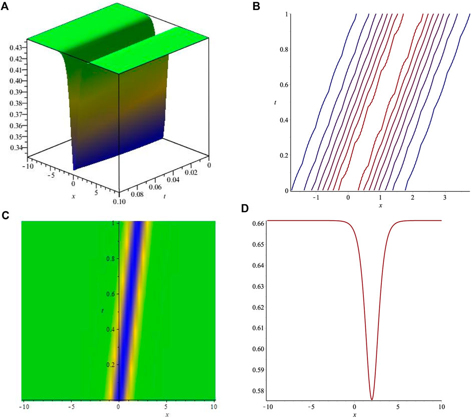
FIGURE 1. Graphical representations of $||{\mathrm{\Lambda }}_2^1(x,t){\Vert }^2$ for c =2.1, μ =2.1, and the remaining arbitrary constants are assigned the value of 1.

FIGURE 2

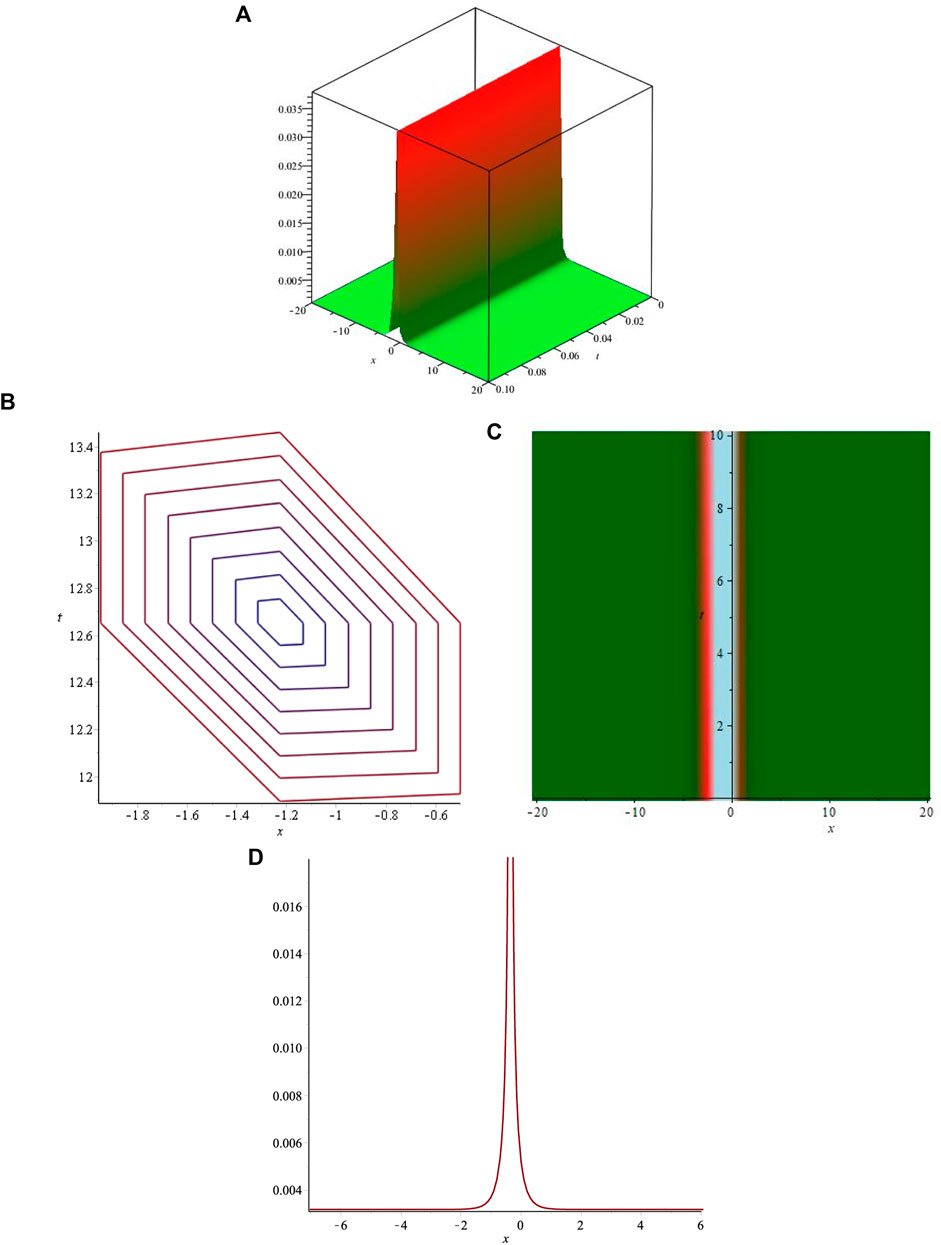
FIGURE 2. Graphical representations of $\Vert {\mathrm{\Lambda }}_2^8(x,t){\Vert }^2$ for c₁= ϵ = D = a = b = ϑ₁= κ =0.11, and the remaining arbitrary constants are assigned the value of 1.

FIGURE 3

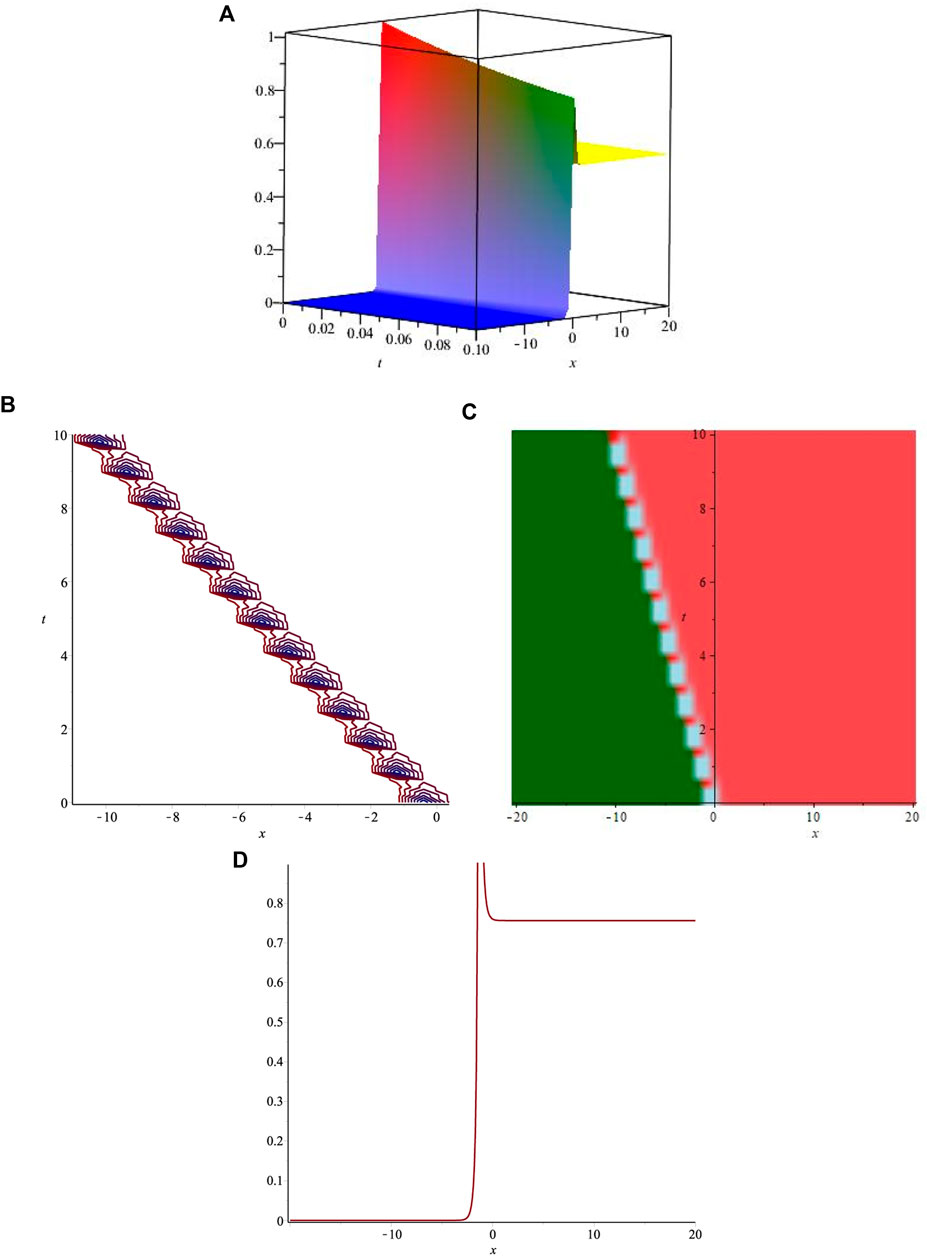
FIGURE 3. Graphical representations of $\Vert {\mathrm{\Lambda }}_2^9(x,t){\Vert }^2$ for D = ϵ = a = b =0.101, ϑ₁=0.9, C =2.1, and the remaining arbitrary constants are assigned the value of 1.

FIGURE 4

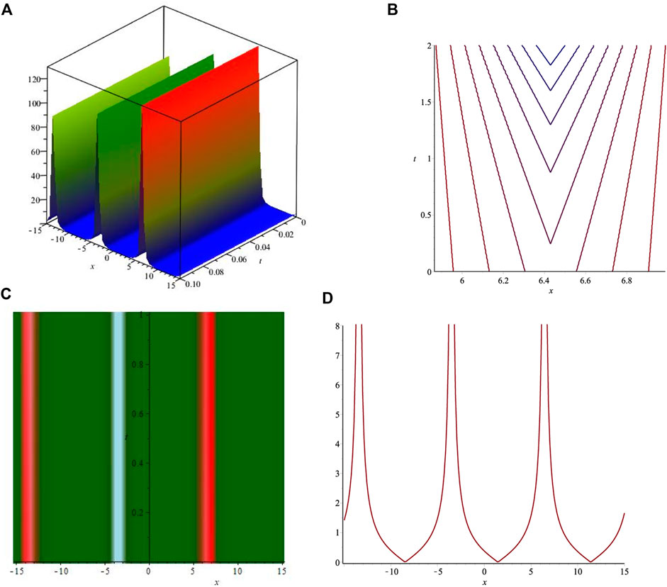
FIGURE 4. Graphical representations of $\Vert {\mathrm{\Lambda }}_1^{10}(x,t){\Vert }^2$ for D = ϵ = a = b =0.101, ϑ₁=0.99, C =2, and the remaining arbitrary constants are assigned the value of 1.

6 Conclusion

The LPD model is investigated in this paper. The exact soliton solutions of the proposed model are obtained by the extended $(\frac{G^{\prime }}{G^2})$-expansion method. The nonlinearity of this model is investigated using three laws of nonlinearity, namely, Kerr law, parabolic law, and anti-cubic law. Many novel solutions are obtained inducing dark, bright, kink, and singular soliton solutions. These optical solitons are successfully retrieved due to the balance of nonlinear effects and dispersion. Based on 3D-surface graphs, 2D contour graphs, density graphs, and 2D-line graphs of acquired soliton solutions, the dynamical behavior of the acquired solutions is discussed. The bright and dark solitons are particularly useful in transmission of data over long distances. They are characterized by the localized increase or decrease in the amplitude of the wave. To the best of our knowledge, the considered model is explored using the proposed technique for the first time in this study. The obtained results are compared with the results already available in the literature using different methods. The retrieved solutions include novel as well as already reported wave solutions of the LPD model showing the reliability of the obtained results. It is evident from the comparison of the results that the present study provides more useful results and a variety of solitonic behavior for the LPD model. The obtained optical solitons may be useful to understand the propagation of light waves through optical media. These solutions will facilitate in further explorations and analysis of wave solutions in physics and engineering. The reported results are hoped to be beneficial in telecommunications, signal transmission, ocean engineering, and optics.

Data availability statement

The original contributions presented in the study are included in the article/Supplementary Material; further inquiries can be directed to the corresponding authors.

Author contributions

GA: conceptualization, methodology, supervision, validation, and investigation; MS: methodology, validation, formal analysis, investigation, and writing—review and editing; MK: software, visualization, and writing—original draft; SP: software, visualization, writing—original draft, and validation.

Conflict of interest

The authors declare that the research was conducted in the absence of any commercial or financial relationships that could be construed as a potential conflict of interest.

Publisher’s note

All claims expressed in this article are solely those of the authors and do not necessarily represent those of their affiliated organizations, or those of the publisher, the editors, and the reviewers. Any product that may be evaluated in this article, or claim that may be made by its manufacturer, is not guaranteed or endorsed by the publisher.

References

1. Liu M, Li X, Zhao Q. Exact solutions to Euler equation and Navier-Stokes equation. Z Angew Math Phys (2019) 70(2):43–13. doi:10.1007/s00033–019–1088–0

CrossRef Full Text | Google Scholar

2. Akram G, Sadaf M, Khan MAU. Soliton dynamics of the generalized shallow water-like equation in nonlinear phenomenon. Front Phys (2022) 10:140. doi:10.3389/fphy.2022.822042

CrossRef Full Text | Google Scholar

3. Hayashi N, Naumkin PI, Sánchez-Suárez I. Asymptotics for the modified witham equation. Commun Pure Appl Anal (2018) 17(4):1407–48. doi:10.3934/cpaa.2018069

CrossRef Full Text | Google Scholar

4. Alquran M, Alqawaqneh A. New bidirectional wave solutions with different physical structures to the complex coupled Higgs model via recent ansatze methods: Applications in plasma physics and nonlinear optics. Opt Quan Electron (2022) 54:301. doi:10.1007/s11082–022–03685–w

CrossRef Full Text | Google Scholar

5. Younis M, Sulaiman TA, Bilal M, Rehman SU, Younas U. Modulation instability analysis, optical and other solutions to the modified nonlinear Schrödinger equation. Commun Theor Phys (2020) 72(6):065001. doi:10.1088/1572–9494/ab7ec8

CrossRef Full Text | Google Scholar

6. Güner Ö, Bekir A, Karaca F. Optical soliton solutions of nonlinear evolution equations using ansatz method. Optik (2016) 127:131–4. doi:10.1016/j.ijleo.2015.09.222

CrossRef Full Text | Google Scholar

7. Bekir A, Zahran EHM. Optical soliton solutions of the thin-film ferro-electric materials equation according to the Painlevé approach. Opt Quan Electron (2021) 53:118. doi:10.1007/s11082-021-02754-w

CrossRef Full Text | Google Scholar

8. Shehata MSM, Rezazadeh H, Jawad AJM, Zahran EHM, Bekir A. Optical solitons to a perturbed Gerdjikov-Ivanov equation using two different techniques. Rev Mex Fis (2021) 67:050704. doi:10.31349/RevMexFis.67.050704

CrossRef Full Text | Google Scholar

9. Tala-Tebue E, Tetchoka-Manemo C, Rezazadeh H, Bekir A, Chu YM. Optical solutions of the (2 + 1)-dimensional hyperbolic nonlinear Schrödinger equation using two different methods. Results Phys (2020) 19:103514. doi:10.1016/j.rinp.2020.103514

CrossRef Full Text | Google Scholar

10. Sabi’u J, Tala-Tebue E, Rezazadeh H, Arshed S, Bekir A. Optical solitons for the decoupled nonlinear Schrödinger equation using Jacobi elliptic approach. Commun Theor Phys (2021) 73:075003. doi:10.1088/1572–9494/abfcb1

CrossRef Full Text | Google Scholar

11. Ali M, Alquran M, Salman OB. A variety of new periodic solutions to the damped (2+1)-dimensional Schrodinger equation via the novel modified rational sine–cosine functions and the extended tanh–coth expansion methods. Results Phys (2022) 37:105462. doi:10.1016/j.rinp.2022.105462

CrossRef Full Text | Google Scholar

12. Alquran M. New interesting optical solutions to the quadratic-cubic Schrödinger equation by using the Kudryashov-expansion method and the updated rational sine-cosine functions. Opt Quan Electron (2022) 54:666. doi:10.1007/s11082–022–04070–3

CrossRef Full Text | Google Scholar

13. Lakshmanan M, Porsezian K, Daniel M. Effect of discreteness on the continuum limit of the Heisenberg spin chain. Phys Lett A (1998) 133(9):483–8. doi:10.1016/0375–9601(88)90520–8

CrossRef Full Text | Google Scholar

14. Al Qarni AA, Alshaery AA, Bakodah HO. Optical solitons for the Lakshmanan-Porsezian-Daniel model by collective variable method. Results Opt (2020) 1:100017. doi:10.1016/j.rio.2020.100017

CrossRef Full Text | Google Scholar

15. Biswas A, Yildirim Y, Yasar E, Zhou Q, Moshokoa SP, Belic M. Optical solitons for Lakshmanan-Porsezian-Daniel model by modified simple equation method. Optik (2018) 160:24–32. doi:10.1016/j.ijleo.2018.01.100

CrossRef Full Text | Google Scholar

16. Akram G, Sadaf M, Khan MAU. Abundant optical solitons for Lakshmanan–Porsezian–Daniel model by the modified auxiliary equation method. Optik (2022) 251:168163. doi:10.1016/j.ijleo.2021.168163

CrossRef Full Text | Google Scholar

17. Akram G, Sadaf M, Khan MAU. Soliton solutions of Lakshmanan–Porsezian–Daniel model using modified auxiliary equation method with parabolic and anti-cubic law of nonlinearities. Optik (2022) 252:168372. doi:10.1016/j.ijleo.2021.168372

CrossRef Full Text | Google Scholar

18. Manafian J, Foroutan M, Guzali A. Applications of the ETEM for obtaining optical soliton solutions for the Lakshmanan-Porsezian-Daniel model. Eur Phys J Plus (2017) 132(11):494–22. doi:10.1140/epjp/i2017–11762–7

CrossRef Full Text | Google Scholar

19. Hubert MB, Betchewe G, Justin M, Doka SY, Crepin KT, Biswas A, et al. Optical solitons with Lakshmanan–Porsezian–Daniel model by modified extended direct algebraic method. Optik (2018) 162:228–36. doi:10.1016/j.ijleo.2018.02.091

CrossRef Full Text | Google Scholar

20. Qarni AA, Banaja MA, Bakodah HO, Alshaery AA, Zhou Q, Biswas A, et al. Bright optical solitons for Lakshmanan–Porsezian–Daniel model with spatio-temporal dispersion by improved Adomian decomposition method. Optik (2019) 181:891–7. doi:10.1016/j.ijleo.2018.12.172

CrossRef Full Text | Google Scholar

21. Akram G, Sadaf M, Arshed S, Sameen F. Bright, dark, kink, singular and periodic soliton solutions of Lakshmanan–Porsezian–Daniel model by generalized projective Riccati equations method. Optik (2021) 241:167051. doi:10.1016/j.ijleo.2021.167051

CrossRef Full Text | Google Scholar

22. Mahak N, Akram G. Analytical solutions to the nonlinear space–time fractional models via the extended (G'/G²)-expansion method-expansion method. Indian J Phys (2020) 94(8):1237–47. doi:10.1007/s12648–019–01554–z

CrossRef Full Text | Google Scholar

23. Akkilic AN, Sulaiman TA, Bulut H. Applications of the extended rational sine-cosine and sinh-cosh techniques to some nonlinear complex models arising in mathematical physics. Appl Math Nonlinear Sci (2021) 6(2):19–30. doi:10.2478/amns.2021.1.00021

CrossRef Full Text | Google Scholar

24. Srivastava HM, Baleanu D, Machado JAT, Osman MS, Rezazadeh H, Arshed S, et al. Traveling wave solutions to nonlinear directional couplers by modified Kudryashov method. Phys Scr (202) 95(7):075217. doi:10.1088/1402–4896/ab95af

CrossRef Full Text | Google Scholar

25. Akram G, Zainab I. Dark Peakon, Kink and periodic solutions of the nonlinear Biswas–Milovic equation with Kerr law nonlinearity. Optik (2020) 208:164420. doi:10.1016/j.ijleo.2020.164420

CrossRef Full Text | Google Scholar