Contrastive Graph Learning for Social Recommendation

1 Introduction

With the rapid development of networks, it is becoming harder and harder for a user to extract useful information from a mass of redundant information. Recommender systems play an important role in solving this problem and have become a promising solution for enhancing economic benefits in many domains like e-commerce, social media, and advertising [1, 2]. The main task of recommender systems is to provide interesting items for each user, which saves a lot of time for users and increases turnover for companies. One of the most popular recommendation techniques is collaborative filtering (CF), which infers each user’s interests to items based on collaborative behaviors of all users without requiring the creation of explicit user and item profiles [3]. Matrix factorization (MF) is a key component in most learnable CF models [4, 5], which decomposes the user–item interaction matrix into two low-dimensional latent matrices for user and item representations [6]. However, MF-based models do not encode user and item embeddings well as a result of insufficient collaborative signals. To yield satisfactory embeddings for CF, a graph neural network (GNN) [7] has been successfully applied to recommender systems [8–10]. Due to the high-order connectivity of GNN [11], GNN-based models can mine collaborative signals including high-order neighbors from abundant historical interactions; thus, it can generate more powerful node representations. But in real-world scenarios, it is always very hard to collect enough historical interaction information. To overcome the problem of data sparsity, many prior CF models [12–14] combine social information with historical interaction information and thus upgrade the recommendation performance. Recently, to further solve the data sparsity, many studies introduced self-supervised learning into recommender systems. The most popular self-supervised learning technology is contrastive learning, which has been successfully employed in many fields [15–18]. Contrastive learning utilizes self-supervision signals in a contrastive way, which pulls positive signals and target embeddings together and pushes negative signals and target embeddings away. To achieve better recommendation performance, many existing recommendation models [19–21] encode node embeddings by a GNN framework and simultaneously resort to contrastive learning in the learning process. Though these models take “social recommendation” as one of their aims, they still have the following inherent limitations that need to be addressed [13].

Firstly, existing GNN-based models [11, 22] learn representations of users and items in the same way and do not consider the different sparsities of users and items. In real-world scenarios, users and items are usually different in number or sparsity. For instance, in the Flickr dataset [23, 24], the number of items is almost 10 times that of users. Due to the huge difference in sparsity, high-quality representations of users may be obtained earlier than items in the learning stage. Thus, representations of users and items learned in the same way might decrease the embedding quality and then degrade the recommendation performance of models.

Secondly, although some social recommendation studies have made efforts to combine contrastive learning and social behaviors, it is still difficult to apply contrastive learning to social recommendation in an appropriate way. On the one hand, existing social recommendation models [19, 25] utilize contrastive learning in a quite complex manner such as encoding hypergraph and data augmentation. This complex manner may destroy the original social graph structure and waste social information. On the other hand, existing social recommendation models [19, 25] do not directly utilize social information in the prediction process, which might reduce the influence of social information. In a word, existing contrastive learning manners increase the complexity of social recommendation models but do not make full use of useful information contained in social behaviors.

This paper explores how to overcome the above limitations in existing recommendation models based on GNN and contrastive learning and proposes a contrastive graph learning (CGL) model for social recommendation. In social recommender systems, there are two kinds of neighbors for each user: historically interacted items and interacted users. Generally speaking, users with similar preferences are more likely to be friends with each other in daily life; likewise, intimate friends often have similar preferences. Hence, it is reasonable to characterize each user’s preference by item aggregation and friend aggregation separately and to require user representations learned from the two views (user–item graph or user–user graph) to have consistent agreement [26]. This argument motivates us to simplify the contrastive learning task between social user embeddings and interest user embeddings. Moreover, to ensure that social user embeddings take part in the prediction process as well, we learn user embeddings in a diffused way inspired by some diffusion models [9, 24]. At each layer in the diffusion process, integrated user embeddings are obtained by taking the average value of social user and interest user embeddings. Besides, to avoid the negative effect of different sparsities in users and items [27], we design an asymmetrical readout strategy for users and items, which takes the average value of user embeddings from all diffusion layers and item embeddings from the last diffusion layer as their readouts, respectively. Since the task of our model is to find out the right items for users instead of mining potential social friends, we set up an extra interest graph for the final aggregation at the end of our model. Therefore, it is very essential to assure that historically interacted behaviors have a more powerful effect on recommendation results than social behaviors.

To summarize, this work makes the following main contributions:

• We successfully combine social information and interaction information by contrastive learning in recommender systems, which significantly improves the quality of recommendation results.

• We design a new readout strategy to alleviate the imbalance problem in the sparsity of users and items, which takes the average value of user embeddings from all layers and item embeddings from the last layer in the diffusion process as their readouts, respectively.

• We construct a pointwise loss between users and items in a contrastive way, which provides positive and negative signals for items. We place this loss and a pairwise loss in different modules to further promote the recommendation performance.

• We compare the proposed model with six state-of-the-art baselines on three real-world datasets, and experimental results demonstrate the effectiveness of our model.

The rest of our paper is organized as follows. Section 2 summarizes some related works in recommender systems. Section 3 introduces necessary notations and describes our model. In Section 4, we give some experimental results to validate the effectiveness of the proposed model and analyze the effect of hyper-parameters. Section 5 concludes our work and discusses some possible issues in future work.

2 Related Work

We simply review MF-based recommendation models and GNN-based recommendation models.

2.1 MF-Based Recommendation

In recommender systems, many classic collaborative filtering algorithms fall into the class of matrix factorization (MF) [28]. MF-based models project users and items into a low-dimensional latent space and represent a user or an item by a vector [29]. The inner product of a user vector and an item vector represents the user’s satisfaction degree to the item. MF-based models have been widely used as baselines in recommender systems. SocialMF [30] employs the MF technique in social networks and assumes each user’s features are dependent on his/her direct neighbors. So the feature vector of each user is supposed to keep consistent with social neighbors. TrustMF [31] considers a twofold influence of trust propagation, which analyzes different implications between truster to trustee and trustee to truster. To take advantage of these two different effects on performance, TrustMF also proposes a synthetic strategy to combine the truster model with the trustee model [32]. NeuMF [33] is the first model that combines the linearity of MF with the nonlinearity of the neural network. It indicates the importance of pre-training in the combination of two different models and achieves better performance than MF-based models and deep neural network (DNN)-based models. DASO [34] dynamically learns representations of users and items by using the generative adversarial network (GAN) [35].

2.2 GNN-Based Recommendation

In recent years, GNNs have shown their effectiveness in the recommendation field. GNNs aim to learn an embedding for each node which contains the information of neighbors [36, 37]. As the simplest GNN, LightGCN [22] does not have any complex operations other than neighbor aggregation, but it still achieves state-of-the-art performance for recommendation. In social recommender systems, GNN is first used in GraphRec [38]. In this model, the attention mechanism is extensively applied to aggregate neighbor information. After the aggregation process, rating scores can be obtained by putting user and item embeddings into a DNN. ConsisRec [39] takes social inconsistency into consideration and categorizes it into the context level and relation level. To solve the inconsistency at the context level, it obtains consistency scores by calculating the distance between neighbor embeddings and query embeddings and then samples consistent neighbors by relating sampling probability with consistency scores. After that, the attention mechanism is adopted to solve the inconsistency at the relation level. DiffNet++ [24] builds a unified framework to diffuse the social influence of social networks and interest influence of interest networks. Because information from social networks and interest networks can be spread into each other, it can receive different information in a recursive way, thereby learning more powerful representations of graph nodes. SGL [26] first introduces contrastive learning to recommendation and improves the accuracy and robustness of GNNs for recommendation. SGL generates graphs with different views by changing the graph structure in different manners and then utilizes supervised signals generated from these views to set an auxiliary self-supervised learning task. SEPT [19] adopts contrastive learning to social recommendation. It builds three different views by data augmentation, and each view provides supervision signals to other views. It employs contrastive learning for social recommendation for the first time, which takes recommendation and contrastive learning as the primary task and auxiliary task, respectively.

3 CGL Model

In this section, we present our CGL model. An overview of CGL is illustrated in Figure 1, which takes a user and an item as an example. CGL consists of three modules with different functions. The first one is a diffusion module, which builds connections between interest interactions and social links and guides the learning of representations in a recursive way. The second one is a readout module, which constructs user embeddings and item embeddings in an asymmetrical way to avoid the imbalance problem of users and items. The third one is a prediction module, which generates recommendations for users.

FIGURE 1

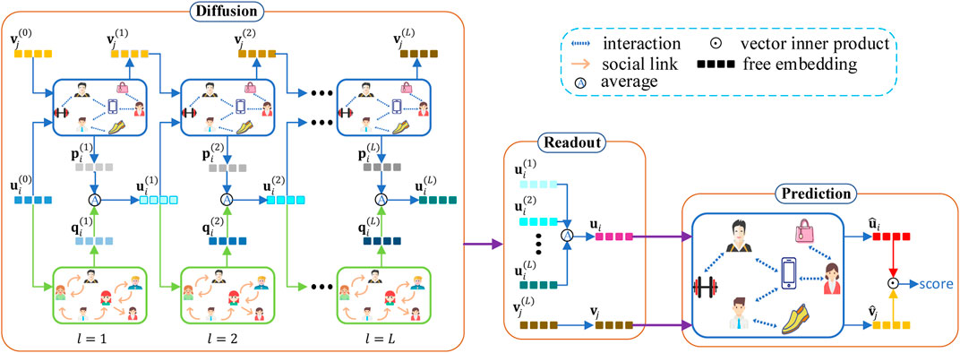
FIGURE 1. The overall architecture of the proposed model.

Some necessary notations are defined in Section 3.1. Section 3.2, Section 3.3, and Section 3.4 introduce the diffusion module, readout module, and prediction module, respectively. The training of the model is given in Section 3.5. Finally, the complexity of CGL is analyzed in Section 3.6.

3.1 Notations

To facilitate the reading, matrices appear in bold capital letters and vectors appear in bold lowercase letters. Let $\mathcal{U}$ and $\mathcal{V}$ be the set of m users and n items, respectively. Denote by ${\mathcal{G}}_r=(\mathcal{N},{\mathcal{E}}_r)$ the user–item interest graph, where $\mathcal{N}$ = $\mathcal{U}\cup \mathcal{V}$ and ${\mathcal{E}}_r$ is the edge set indicating interactions between users and items. Let ${\mathcal{G}}_s=(\mathcal{T},{\mathcal{E}}_s)$ be the user–user social graph, where $\mathcal{T}\subseteq \mathcal{U}$ and ${\mathcal{E}}_s$ is the edge set indicating social links among users. In this paper, we keep all users in a social network, so $\mathcal{T}=\mathcal{U}$. For ${\mathcal{G}}_r$, the binary matrix $\mathbf{R}={[r_{ij}]}_{m\times n}$ represents its user–item interactions, where r_ij = 1 if user i has an interaction with item j; otherwise, r_ij = 0. For ${\mathcal{G}}_s$, the binary matrix $\mathbf{S}={[s_{ij}]}_{m\times m}$ represents its user–user social links, where s_it = 1 if user i has a link with another user t; otherwise, s_it = 0.

For users and items, we encode two basic embedding matrices, ${\mathbf{U}}^{(0)}=[{\mathbf{u}}_1^{(0)},{\mathbf{u}}_2^{(0)},\dots ,{\mathbf{u}}_{|\mathcal{U}|}^{(0)}]$ and ${\mathbf{V}}^{(0)}=[{\mathbf{v}}_1^{(0)},{\mathbf{v}}_2^{(0)},\dots ,{\mathbf{v}}_{|\mathcal{V}|}^{(0)}]$, where ${\mathbf{u}}_i^{(0)}$ is a d-dimensional embedding of user i and ${\mathbf{v}}_j^{(0)}$ is a d-dimensional embedding of item j. Starting from U⁽⁰⁾ and V⁽⁰⁾, a graph convolution operation is implemented on ${\mathcal{G}}_r$ and ${\mathcal{G}}_s$ to produce user and item representations, respectively.

3.2 Diffusion Module

The diffusion module has L layers, and each layer consists of aggregation on the interest graph, aggregation on the social graph, and their integration. The input of the first layer is the initialized user latent embedding ${\mathbf{u}}_i^{(0)}$ and item latent embedding ${\mathbf{v}}_j^{(0)}$, and the input of other layers is the output of their respective previous layers. These layers recursively model the user’s latent preference and the item’s latent preference propagation in two graphs with layer-wise convolutions. LightGCN [22] is a brief graph convolution network (GCN)-based general recommendation model, which discards two standard operations in GCNs: feature transformation and nonlinear activation. We utilize LightGCN to realize aggregation operations in CGL.

To aggregate interaction information in the interest graph ${\mathcal{G}}_r$, we collect the neighbor information of each node by the simple way of LightGCN. Specifically, for a given user i and item j, let ${\mathbf{u}}_i^{(l-1)}$ and ${\mathbf{v}}_j^{(l-1)}$ represent user embedding and item embedding from the (l − 1)-th layer, respectively. Then the l-th layer interest aggregation process is given by

${\mathbf{p}}_i^{\left(l\right)}=Ag{g}_{items}\left({\mathbf{v}}_j^{\left(l-1\right)},\forall j\in {\mathcal{N}}_i\right)=\sum _{j\in {\mathcal{N}}_i}\frac{{\mathbf{v}}_j^{\left(l-1\right)}}{\sqrt{|{\mathcal{N}}_i\Vert {\mathcal{N}}_j|}},(1)$

${\mathbf{v}}_j^{\left(l\right)}=Ag{g}_{users}\left({\mathbf{u}}_i^{\left(l-1\right)},\forall i\in {\mathcal{N}}_j\right)=\sum _{i\in {\mathcal{N}}_j}\frac{{\mathbf{u}}_i^{\left(l-1\right)}}{\sqrt{|{\mathcal{N}}_j\Vert {\mathcal{N}}_i|}},(2)$

where ${\mathcal{N}}_i$ is the set of items that are interacted by user i and ${\mathcal{N}}_j$ is the set of users that interact with item j. LightGCN keeps the same normalization operation as standard GCNs [40]; i.e., the neighbor number of the current node and aggregated node is utilized for normalization during aggregating information. This strategy is rather essential to avoid the unreasonable increase of embedding in graph convolution operations.

To aggregate social information of the social graph ${\mathcal{G}}_s$, we perform node aggregation based on LightGCN as well. Note that there are only user nodes in social graphs. Let ${\mathbf{u}}_i^{(l-1)}$ and ${\mathcal{T}}_i$ be user embeddings from the (l − 1)-th layer and the set of social neighbors linked with user i, respectively. The l-th layer social aggregation process is defined by

${\mathbf{q}}_i^{\left(l\right)}=Ag{g}_{neighbors}\left({\mathbf{u}}_t^{\left(l-1\right)},\forall t\in {\mathcal{T}}_i\right)=\sum _{t\in {\mathcal{T}}_i}\frac{{\mathbf{u}}_t^{\left(l-1\right)}}{\sqrt{|{\mathcal{T}}_i\Vert {\mathcal{T}}_t|}}.(3)$

As the above equation shows, LightGCN designs normalization by taking the neighbor number of current trustee node and aggregated truster node.

Aggregation on the interest graph generates user embedding ${\mathbf{p}}_i^{(l)}$ and aggregation on the social graph produces user embedding ${\mathbf{q}}_i^{(l)}$. These two user embeddings contain different information about user i and will be further integrated to generate user embedding ${\mathbf{u}}_i^{(l)}$ at the l-th layer. We simply integrate ${\mathbf{p}}_i^{(l)}$ and ${\mathbf{q}}_i^{(l)}$ by taking their average value. That is to say, we get integrated user embedding at the l-th layer by

${\mathbf{u}}_i^{\left(l\right)}=\frac{{\mathbf{p}}_i^{\left(l\right)}+{\mathbf{q}}_i^{\left(l\right)}}{2}.(4)$

Then integrated user embedding ${\mathbf{u}}_i^{(l)}$ and aggregated item embedding ${\mathbf{v}}_j^{(l)}$ are input into the (l + 1)-th layer so as to diffuse interest and social information into two graphs. By integrating social user embeddings and interest user embeddings at each layer, we can update integrated user embeddings consecutively. Consequently, the fusion between social information and interest information becomes closer and closer in the convolution process. Moreover, although item embeddings do not take part in the diffusion process, due to the high-order connectivity in GNN, social user embeddings and item embeddings can still exert a powerful influence on each other, especially when the diffusion process becomes deeper.

The diffusion process of CGL is inspired by the validity of the diffusion model DiffNet++, but it is much more concise than that of DiffNet++. Unlike the Diffnet++, CGL does not absorb any information from other attribute features of users or items and introduce any attention mechanism. The former will take us a lot of time to process attribute features, and the latter will use DNNs. As such, the time complexity of our diffusion process is lower compared with that of DiffNet++.

3.3 Readout Module

After the above L layer diffusion process, we construct readouts for users and items, separately, and then these readouts are sent to the last interest graph in the subsequent prediction module. Our strategy for constructing readouts is different from existing GNN-based recommendation models. In existing GNN-based models, there are two strategies to prepare embeddings for the prediction phase or other subsequent phases. One is taking the average value of all layers’ embeddings for users and items, and the other is taking the embedding value of the last stacked layer. Both these strategies deal with users and items in a symmetrical manner, which results in the model being unable to learn good representations of users and items while the numbers of users and items in the training data are very different. To alleviate the problem, we integrate these two strategies to constitute readouts of users and items and adopt the former for users and the latter for items. Because of the massive use of social information, user embeddings in each layer of the diffusion process contain some collaborative signals, which can improve the quality of user embeddings. Thus high-quality representations of users may be generated in early stages of the diffusion process. That encourages us to use all user embeddings in the diffusion process to build readouts of users. Specifically, the readout u_i of user i is defined as the average of embeddings from all L layers in the diffusion process:

${\mathbf{u}}_i=Rdou{t}_{users}\left(\left\{{\mathbf{u}}_i^{\left(l\right)}|l=\left[1,\dots ,L\right]\right\}\right)=\frac{1}{L}\sum _{l=1}^L{\mathbf{u}}_i^{\left(l\right)}.(5)$

For an item, its embedding in the early stage of the diffusion process may be poor due to the large item number, sparsity, and lack of auxiliary information. So the readout v_j of item j is defined as its embedding at the last layer in the diffusion process:

${\mathbf{v}}_i=Rdou{t}_{items}\left(\left\{{\mathbf{v}}_i^{\left(l\right)}|l=\left[1,\dots ,L\right]\right\}\right)={\mathbf{v}}_j^{\left(L\right)}.(6)$

From Eq. 5 and Eq. 6, it can be seen that our readout strategy is asymmetrical for users and items.

3.4 Prediction Module

Considering that the task of recommendation is to predict interactions between users and items, we add a separate interest graph to emphasize the influence of interaction information between their readouts. The interest graph generates the final user embedding ${\widehat{\mathbf{u}}}_i$ and item embedding ${\widehat{\mathbf{v}}}_j$ by aggregating v_js and u_is, respectively. That is,

${\widehat{\mathbf{u}}}_i=Ag{g}_{items}\left({\mathbf{v}}_j,\forall j\in {\mathcal{N}}_i\right),(7)$

${\widehat{\mathbf{v}}}_j=Ag{g}_{users}\left({\mathbf{u}}_i,\forall i\in {\mathcal{N}}_j\right).(8)$

Then the prediction module defines the inner product between the final user and item embeddings

${\widehat{r}}_{ij}=<{\widehat{\mathbf{u}}}_i,{\widehat{\mathbf{v}}}_j>.(9)$

The inner product is taken as the ranking score to generate recommendations.

3.5 Model Training

To train the model, we design a self-supervised loss for the diffusion module and a supervised loss for the readout module and prediction module. At each layer of the diffusion module, the interest graph and social graph generate two user embeddings for each user separately. In order to make the integration on them more reasonable, we design a self-supervised loss to close two embeddings of the same user. Users and items are two aspects of recommender systems, and we can recommend items for a given user or select users for a given item. According to these two tasks, we design a supervised loss in the readout module and prediction module, respectively. By jointly optimizing the above three losses, we learn parameters in the model.

3.5.1 Self-Supervised Loss

We integrate social user embeddings and interest user embeddings by Eq. 4 at each layer of the diffusion process. Such a direct integration strategy can make the two groups of embeddings complement each other but cannot guarantee that they know each other in the training process. So, we introduce a social contrastive learning loss in the diffusion module. The main idea comes from the assumption that social behaviors can usually reflect the preference of a user. As a result, the user’s embedding from the social graph is supposed to have a close connection with that from the interest graph.

For convenience, let ${\mathbf{P}}^{(l)}=[{\mathbf{p}}_1^{(l)},{\mathbf{p}}_2^{(l)},\dots ,{\mathbf{p}}_{|\mathcal{U}|}^{(l)}]\in {\mathbb{R}}^{m\times k}$ be the l-th interest aggregation matrix on the interest graph, where ${\mathbf{p}}_i^{(l)}$ is calculated by Eq. 1. Similarly, ${\mathbf{Q}}^{(l)}=[{\mathbf{q}}_1^{(l)},{\mathbf{q}}_2^{(l)},\dots ,{\mathbf{q}}_{|\mathcal{V}|}^{(l)}]\in {\mathbb{R}}^{m\times k}$ denote the l-th social aggregation matrix, where ${\mathbf{q}}_i^{(l)}$ is calculated by Eq. 3. We first produce two user embedding matrices P and Q by

$\mathbf{P}=\frac{{\sum }_{l=1}^L{\mathbf{P}}^{\left(l\right)}}{L},(10)$

$\mathbf{Q}=\frac{{\sum }_{l=1}^L{\mathbf{Q}}^{\left(l\right)}}{L}.(11)$

We randomly ruffle matrix Q row-wise and column-wise in turn and denote the ruffled one as $\tilde{\mathbf{Q}}$

$\tilde{\mathbf{Q}}=r\left(\mathbf{Q}\right),(12)$

where r(⋅) is the ruffle operation. Then the i-th row of the user embedding matrix can be a latent embedding of user i, and the j-th row of the item embedding matrix can be a latent embedding of item j. Thus, for user i and item j, we can get the interest user embedding p_i from P, real social user embedding q_i from Q, and fake social user embedding ${\tilde{\mathbf{q}}}_i$ from $\tilde{\mathbf{Q}}$. We assume that fake social user embeddings are quite different from their corresponding interest user embeddings. We minimize the agreement between each fake social user embedding and its corresponding interest user embedding, and the social contrastive learning loss in the diffusion module can be formulated as

${\mathcal{L}}_{c-uu}=\sum _{i\in \mathcal{U}}-\left(\mathit{log}\left(\sigma \left(<{\mathbf{p}}_i,{\mathbf{q}}_i>\right)\right)+\mathit{log}\left(1-\sigma \left(<{\mathbf{p}}_i,{\tilde{\mathbf{q}}}_i>\right)\right)\right),(13)$

where σ(⋅) is the sigmoid function.

3.5.2 Supervised Loss

In the prediction module, we can get rating scores by Eq. 9. To assure observed interactions can achieve higher scores than unobserved interactions, we employ the pairwise Bayesian personalized ranking (BPR) loss as our primary loss to induce model learning, which is proposed to make the observed interactions be ranked in front of unobserved interactions. The BPR loss in CGL is formulated as

${\mathcal{L}}_{bpr}=\sum _{\left(i,j^{+},j^{-}\right)\in \mathcal{R}}-\mathit{log}\left(\sigma \left({\widehat{r}}_{i{j}^{+}}-{\widehat{r}}_{i{j}^{-}}\right)\right),(14)$

where $\mathcal{R}=\{(i,j^{+},j^{-})|(i,j^{+})\in R^{+},(i,j^{-})\in R^{-}\}$ denotes training data, R⁺ indicates observed interactions, and R⁻ indicates unobserved interactions. By minimizing the BPR loss, the predictive score of an observed interaction could be enforced to be higher than that of its unobserved counterparts. However, as a pairwise loss, it ignores the entrywise consistency between predictive scores and real scores. Besides, the BPR loss only provides positive and negative signals for a given user, which is unfair for items and makes it hard to learn good item representations.

To overcome this shortcoming, we employ a pointwise loss as a complement to the BPR loss and formulate it as

${\mathcal{L}}_{c-uv}=\sum _{j\in \mathcal{V}}\sum _{i\in {\mathcal{N}}_j}-\mathit{log}\frac{\exp \left(<{\mathbf{u}}_i,{\mathbf{v}}_j>\right)}{\sum _{t\in \mathcal{U}}\exp \left(<{\mathbf{u}}_t,{\mathbf{v}}_j>\right)},(15)$

where each u_i and v_j are given by Eqs 5 and 6, respectively. Obviously, this loss provides positive and negative supervised signals for a given item, instead of a given user. By minimizing Eq. 15, predictive scores could be consistent with real scores. It is worth mentioning that we define the loss in the readout module instead of in the prediction module. This is different from most existing heterogeneous losses that typically combine the pointwise loss and pairwise loss in the prediction module. The main reason is that we separate the predictive task and the ranking task by using different user and item representations. The pointwise loss focuses on users for a given item and enhances the user representation directly derived from the aggregation operation on both interest and social graphs. And these enhanced user and item representations are used to aggregate information on an interest graph for the ranking task.

3.5.3 Final Loss

With the above three losses in three modules of the CGL model, we set its final loss as

${\mathcal{L}}_{CGL}={\mathcal{L}}_{bpr}+\alpha {\mathcal{L}}_{c-uu}+\beta {\mathcal{L}}_{c-uv}+\lambda \Vert \mathrm{\Theta }{\Vert }_2^2,(16)$

where α and β are two additional regularizers to control the strength of ${\mathcal{L}}_{c-uu}$ and ${\mathcal{L}}_{c-uv}$, respectively; Θ is the set of all learnable parameters; and λ controls the strength of L₂ regularization. The overall training process of CGL is given in Algorithm 1.

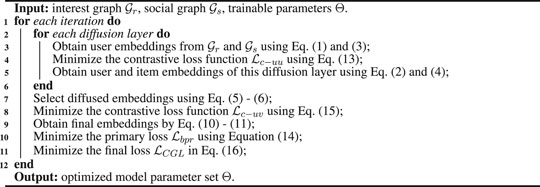
Algorithm 1. The training process of CGL.

3.6 Complexity Analysis

The overall time complexity of CGL mainly comes from two parts: aggregation on graphs and calculation on three losses. At each iteration, training data aggregate neighbor information on interest graphs L + 1 times and on social graphs L times. Thus, the complexity of aggregation on interest graphs is $\mathcal{O}(|\mathbf{R}|d(L+1))$, which is only dependent on the latent dimension and the size of rating data. Similarly, the complexity of aggregation on social graphs is $\mathcal{O}(|\mathbf{S}|dL)$. Compared with interest aggregation, besides the difference in aggregation number, social aggregation has fewer nodes in the graph structure. In short, the time complexity of the aggregation operation on graphs increases linearly with the size of training data, the dimension of latent embedding, and the number of aggregation. For the complexity of calculation on three losses, we only take the inner product operation into consideration, since it produces the major complexity in our model. Within a batch, the complexity of the contrastive loss ${\mathcal{L}}_{c-uu}$ is $\mathcal{O}(2Bd)$, where B is the batch size. For another contrastive learning loss ${\mathcal{L}}_{c-uv}$, we get its numerator by calculating the inner product between each positive pair in a batch; hence, the complexity of the numerator is $\mathcal{O}(Bd)$. Likewise, the denominator is obtained by the product between the user embedding matrix and item embedding matrix, and its complexity is $\mathcal{O}(B^{2}d)$. For the BPR loss, we calculate the inner product of all positive pairs and negative pairs in each batch, and its complexity is $\mathcal{O}(2Bd)$. Therefore, the total time complexity of training CGL in one batch is $\mathcal{O}(|\mathbf{R}|d(L+1)+|\mathbf{S}|dL+5Bd+B^{2}d)$.

4 Experiments

We conduct multiple experiments to verify the effectiveness of CGL in this section. Experimental setup is introduced in Section 4.1. The performance of CGL is compared with six baselines in Section 4.2. Section 4.3 analyzes the effects of different strategies for the readout strategy and pointwise contrastive loss. Section 4.4 shows the performance of CGL under different hyper-parameters. Note that we omit the percent sign of model performance in all tables.

4.1 Experimental Setup

Experimental setup contains datasets, evaluation metrics, baselines, and parameter settings.

4.1.1 Datasets

The task of our experiments is a top-K recommendation, and we conduct experiments on three representative real-world datasets: Yelp [24], Flickr [23], and Ciao [41].

• Yelp: This dataset is crawled from an online location-based review site, Yelp. Users on the site are encouraged to interact with others and express their opinions through the form of reviews and ratings. The ratings data are converted into implicit feedback as the dataset. The itemset of this dataset includes a variety of locations visited or reviewed by users. And the relationship among users can be found out directly in terms of the friend list of users.

• Flickr: This dataset is crawled from one of the largest social image-sharing platforms, Flickr. In this platform, users can share their preferences in images with their social followers and follow the people they are interested in. So, social images make up the itemset, and the social relationship can be confirmed through followers of users.

• Ciao: This dataset is crawled from an online shopping site, Ciao. On the site, people not only write critical reviews for various products but also read and rate the reviews written by others. Furthermore, people can add members to their trust networks or “Circle of Trust”, if they find their reviews consistently interesting and helpful [41]. The itemset of this dataset includes a variety of goods.

The above three datasets can be publicly downloaded online (Yelp and Flickr,¹ and Ciao²) provided by [19, 23], and their statistics are summarized in Table 1. Following many previous works [9, 24], we convert all explicit ratings into implicit ratings and remove repeated ratings in each dataset. Similar to [30], we only focus on the social information in these datasets and do not consider the attribute information of users and items. Finally, we randomly select 10% of rating data as testing set and the rest as training set.

TABLE 1

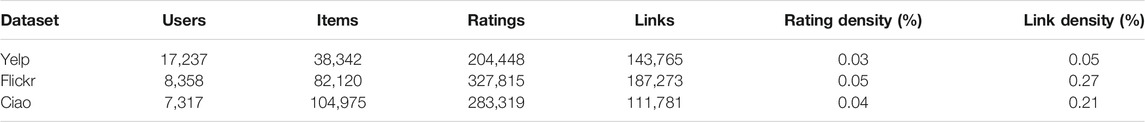
TABLE 1. The statics of datasets.

4.1.2 Evaluation Metrics

For all models, we perform item ranking on all candidate items and evaluate the performance of each model with Precision@K, Recall@K, and NDCG@K metrics, which are three widely used evaluation protocols. The NDCG metric is sensitive to rank, and the other two metrics can measure the relevancy of the recommendation list.

4.1.3 Baselines

• MF-BPR [42]: It exploits how to represent users and items in a low-dimensional latent space, which is optimized by the BPR loss.

• SocialMF [30]: It combines social information and purchase information through the form of MF. For a specific user, this model focuses on not only items purchased by the user but also social neighbors around the user.

• LightGCN [22]: It is a light version of the GNN-based model and only performs aggregation operations. As a state-of-the-art model, it has been widely used as a baseline in many recommender system studies.

• SEPT [19]: It builds complementary views of the raw data so as to provide self-supervision signals (pseudo-labels) to participate in the contrastive learning. To ensure the effectiveness of contrastive learning, it simultaneously employs the tri-training scheme to coordinate the labeling process.

• SGL [26]: It constructs different views by perturbing the raw data graph with uniform node/edge dropout and then conducts self-discrimination-based contrastive learning over these views to learn node representations.

• DiffNet++ [24]: It recursively diffuses different information into social networks and interest networks, which can be used without attribute information fusion and attention mechanism.

4.1.4 Settings

For a fair comparison, all models are optimized by the Adam optimizer [43] and initialized in the same way. The size of each batch is set to 2,048, and the dimension of the latent vector is tuned in {8, 16, 32, 64, 128}. It is worth noting that MF-based models are often different from GNN-based models in L₂ regularization. In order to ensure that all models can achieve good results, the L₂ regularization coefficient λ is chosen from {1.0 × 10^–1, 1.0 × 10^–2} for MF-based models and from {1.0 × 10^–4, 5.0 × 10^–5, 1.0 × 10^–5} for GNN-based models. The learning rate is tuned in {1.0 × 10^–2, 5.0 × 10^–3, 1.0 × 10^–3}, and the maximum train epoch is 150. For α and β, we tune them in different ranges on three datasets. On Yelp, α and β are searched in {4.0 × 10^–4, 4.0 × 10^–5, 4.0 × 10^–6, 4.0 × 10^–7, 4.0 × 10^–8} and {6.5 × 10^–1, 6.5 × 10^–2, 6.5 × 10^–3, 6.5 × 10^–4, 6.5 × 10^–5}, respectively. On Flickr, α and β are tuned in {1.6 × 10^–4, 1.6 × 10^–5, 1.6 × 10^–6, 1.6 × 10^–7, 1.6 × 10^–8} and {8.5 × 10^–5, 8.5 × 10^–6, 8.5 × 10^–7, 8.5 × 10^–8, 8.5 × 10^–9}, respectively. On Ciao, α and β are tuned in {2.0 × 10^–5, 2.0 × 10^–6, 2.0 × 10^–7, 2.0 × 10^–8, 2.0 × 10^–9} and {1.0 × 10^–0, 1.0 × 10^–1, 1.0 × 10^–2, 1.0 × 10^–3, 1.0 × 10^–4}, respectively. Our experiments are implemented in PyTorch.

4.2 Overall Performance Comparison

We evaluate our proposed CGL model by comparing it with six baselines. For all models, we exhibit the performance of the top 10, top 15, and top 20 in Table 2, Table 3, and Table 4, respectively. From these tables, we have the following observations:

• CGL outperforms all baselines on Yelp and Flickr by a large margin. On Yelp, the average top-K (10, 15, 20) improvement of CGL on Precision, Recall, and NDCG is 6.60%, 5.77%, and 6.63%, respectively. On Flickr, the average top-K (10, 15, 20) improvement of CGL on Precision, Recall, and NDCG is 9.76%, 10.80%, and 10.01%, respectively. On Ciao, the average top-K (10, 15, 20) improvement of CGL on Precision, Recall, and NDCG is −2.17%, 3.97%, and 2.06%, respectively. Although CGL’s performance on Ciao is not as good as that on Yelp and Flickr, it is still the best or second best among all models in terms of the three metrics. Since the overall performance of all models is similar when K = 10, K = 15, and K = 20, we only discuss the case of K = 20 in the subsequent experiments.

• Nearly all GNN-based models (e.g., LightGCN, DiffNet++, and SGL) perform much better than MF-based models (MF-BPR and SocialMF), which demonstrates the important role of GNNs for the recommendation task. We also observe that some GNN-based models (DiffNet++ and SEPT) incorporate the social information, but cannot beat other models without social information on some metrics. It illustrates that though social behaviors may reflect a person’s interest information to an item indeed, it is hard to mathematically design a reasonable and effective manner to utilize social information. Fortunately, CGL performs better than almost all baselines, which proves that contrastive learning in CGL can ensure the effectiveness of the social information.

• Compared with its performance on Yelp and Ciao, CGL brings more improvement on Flickr. As Flickr has much denser social information, this may indicate that CGL can make full use of social information. Besides, by analyzing the performance of DiffNet++ and CGL on Ciao, we conclude that there may be much noise in the raw data of Ciao so that it is hard to improve the recommendation performance by directly diffusing social information and interest information. Naturally, SGL shows better performance on some metrics because self-discrimination-based contrastive learning can help to alleviate noise effect greatly.

TABLE 2

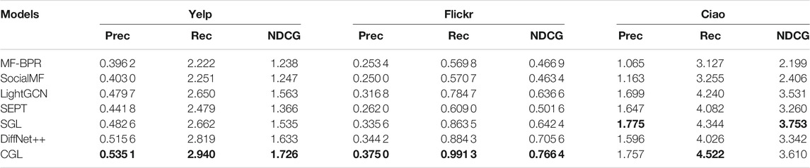
TABLE 2. Overall comparison (K = 10). The best results are in bold.

TABLE 3

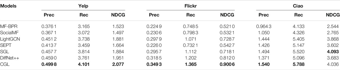
TABLE 3. Overall comparison (K = 15). The best results are in bold.

TABLE 4

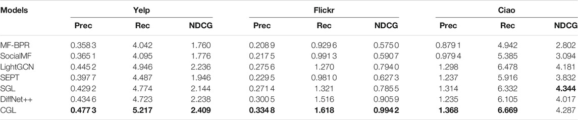
TABLE 4. Overall comparison (K = 20). The best results are in bold.

Moreover, to concretely investigate the impact of contrastive learning and the diffusion process on the model, we further compare CGL with two other GNN-based models (LightGCN and DiffNet++) at each layer and show the relevant results in Table 5 (K = 20). From the table, we have the following observations:

• CGL outperforms LightGCN and DiffNet++ at the first and the third layers on both Yelp and Flickr with respect to all metrics. At the second layer, CGL still achieves the best performance except Recall and NDCG on Flickr. On Ciao, our model reaches its best performance at the first layer, and the performance is better than that of DiffNet++ and LightGCN at any layer. These experiment results illustrate the superiority of our model and the necessity of constructing supervised loss for social user representations.

• The overall performance of LightGCN at each layer is better than that of Diffnet++ on Yelp. However, DiffNet++ performs better than LightGCN on Flickr. A possible reason is that directly diffusing social information without any supervised measure cannot guarantee the validity of social information, especially while social information is inadequate. However, the performance of DiffNet++ is inferior to that of LightGCN on Ciao; we infer there may be much noise in this dataset and it makes a negative effect on the diffusion process. We will further validate our argument in the parameter analysis experiments.

• LightGCN reaches its best performance at the third layer on Yelp and at the second layer on Flickr and Ciao. DiffNet++ has a similar trend with LightGCN at each layer, even though it incorporates social information. CGL achieves its best results at the third layer on Yelp and Flickr and at the first layer on Ciao. The difference between the trend of CGL and the other two models may be attributed to two aspects. Firstly, when there exists few noise in the raw data of rating data and social links, a deeper diffusion layer can help the model extract useful information from them. Secondly, if there exists a lot of noise in the raw data, a deeper diffusion layer will have a negative effect on the model since noise will be diffused at each layer.

TABLE 5

TABLE 5. Comparison of CGL and two GNN-based baselines at each layer (K = 20). The best results at each layer are in bold.

Lastly, we show the runtime of each model on three datasets in Table 6 so as to evaluate the model performance thoroughly. The layer number is set as three for all GNN-based models to assure the fairness of comparison. From Table 6, we can see that the average time of our model for each epoch is about 25 s, which is much less than SEPT and SGL. Considering the excellent performance of CGL, we conclude it is efficient and effective.

TABLE 6

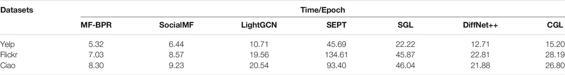
TABLE 6. Average epoch runtime of all models (seconds).

4.3 Component Study

We analyze the impact of the readout strategy and the pointwise loss in the readout module of CGL in this section. For the readout strategy, CGL employs the average values of user embeddings from all layers in the diffusion process and item embeddings from the last layer, which is an asymmetrical manner for users and items and originates from the huge difference in number and sparsity of users and items. To validate the effectiveness of this asymmetrical readout strategy in CGL, its two variants are designed to compare their performance, which uses two common symmetrical readout strategies. One variant is denoted by CGL-M, which takes the average value of user and item embeddings from all layers in the diffusion process as readouts of users and items, respectively. The other is CGL-L, which treats embeddings from the last layer in the diffusion process as readouts of users and items. Experimental results of CGL and its variants on three datasets are given in Table 7 (K = 20).

TABLE 7

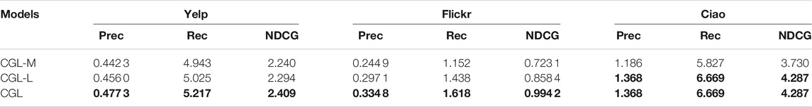
TABLE 7. Comparison of CGL and its variants with different readout strategies (K = 20). The best results are in bold.

From Table 7, we can see that CGL outperforms CGL-M and CGL-L on all three datasets, which indicates the superiority of our asymmetrical readout strategy. Note that the structures of CGL and CGL-L are identical when we fix the layer number at one, which explains why they have the same performance on Ciao (they achieve their best results at the first layer). Moreover, CGL exceeds CGL-M and CGL-L by a bigger margin on Flickr and Ciao than on Yelp. It is worth noting that the imbalance between the number of users and items in Flickr (8,358 vs. 82,120) and Ciao (7,317 vs. 104,975) is much more serious than that in Yelp (17,237 vs. 38,342). So, the bigger margin further demonstrates that the asymmetrical readout strategy in CGL can effectively alleviate the bad effect of the imbalance between users and items.

CGL has a pointwise loss ${\mathcal{L}}_{c-uv}$ in the readout module and a pairwise BPR loss in the prediction module, but existing models usually combine these two losses in the prediction module. To investigate the benefit of placing two losses separately in CGL, we transfer ${\mathcal{L}}_{c-uv}$ together with the BPR loss in the prediction module, take corresponding mode as a CGL variant, and denote it by CGL-P. Experimental results of CGL-P and CGL on all datasets are given in Table 8 (K = 20).

TABLE 8

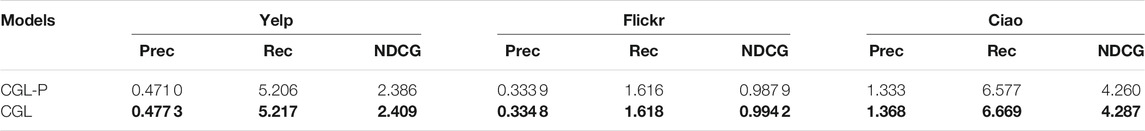
TABLE 8. Comparison of CGL and its variant with different pointwise loss positions (K = 20). The best results are in bold.

From Table 8, we can see that CGL achieves better performance on all datasets with respect to all three metrics compared with CGL-P. This indicates that the performance of CGL is affected by the position of ${\mathcal{L}}_{c-uv}$ and that it is better to put it in the readout module. Actually, the pointwise ${\mathcal{L}}_{c-uv}$ loss and the pairwise BPR loss emphasize different aspects of user and item embeddings, and they should be placed in different positions according to different goals. The pointwise loss focuses on the entrywise consistency between user embeddings and item embeddings, which is used to provide accurate profiles of users and items and should be put before the aggregation in the prediction module. However, the pairwise loss focuses on the consistency between observed and unobserved interactions, which is used to improve ranking performance and should be set after the aggregation in the prediction module.

4.4 Parameter Analysis

Impacts of α, β, and embedding size d on CGL are analyzed, where α and β are two unique parameters of our model to control the strength of contrastive losses ${\mathcal{L}}_{c-uu}$ and ${\mathcal{L}}_{c-uv}$. Experimental results of CGL with different α, β, and d values are given in Table 9, Table 10, and Table 11 (K = 20), respectively. For the simplicity of expression, we omit the coefficient of α (4.0 on Yelp, 2.0 on Ciao, and 6.5 on Flickr) in Table 9 and the coefficient of β (1.6 on Yelp, 1.0 on Ciao, and 8.5 on Flickr) in Table 10.

TABLE 9

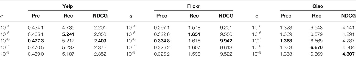
TABLE 9. Performance of CGL with respect to different values of α (K = 20). The best results are in bold.

TABLE 10

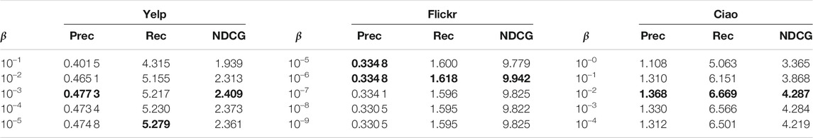
TABLE 10. Performance of CGL with respect to different values of β (K = 20). The best results are in bold.

TABLE 11

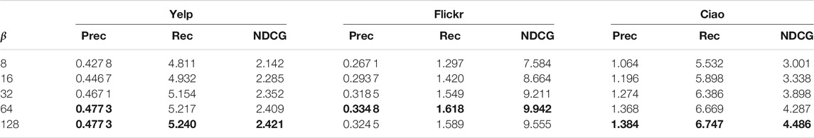
TABLE 11. Performance of CGL with respect to different embedding sizes d (K = 20). The best results are in bold.

From Table 9, we can see that on Yelp and Flickr, all three metrics achieve their peaks while tuning α in its parameter range. This illustrates that ${\mathcal{L}}_{c-uu}$ can have a stable influence on the model even though it faces different sparsities of social information in different datasets. When α is bigger than a certain number (10^–5 for Yelp and Flickr and 10^–7 for Ciao), the performance of CGL degrades. This phenomenon indicates that placing too much emphasis on the consistency between social behaviors and historical interactions will destroy the learning process of model parameters. When α is smaller than 10^–6, CGL generates worse performance on Yelp and Flickr as well. This is because social behaviors and historical interactions can provide supervised signals for each other, and it is unreasonable to set α to be too small. So it is important to find a suitable α value to balance the effect between two behaviors. However, on Ciao, CGL performs well when α is set to be small. This shows evidence that there exists too much noise in the dataset and explains the reason why DiffNet++ performs badly. In general, we suggest to carefully tune α in the range of [10^–5, 10^–7].

From Table 10, we observe that on Yelp all three metrics have relatively large fluctuation ranges while increasing β from 10^–1 to 10^–5 and Recall achieves its best result at a β value (10^–5) quite different from that of Precision and NDCG (10^–3). However, on Flickr and Ciao, all three metrics keep relatively stable, and they achieve their best results at the same β value. Moreover, β is tuned in quite different ranges on three datasets. CGL achieves the best performance at a larger β value on Ciao and Flickr and a smaller value on Yelp. The reason might be that these datasets have different sparsities in rating information. Compared with Yelp and Ciao, Flickr provides denser social information and interest information to train the model, which makes the model insensitive to parameter β and easy to train. On Yelp and Ciao, there is not enough social information or there exists too much noise, so the model depends more on the supervised signals in ${\mathcal{L}}_{c-uv}$. In general, a larger value is suggested for β for sparse datasets and a smaller value for dense datasets. By considering the overall performance, we suggest to carefully choose β in [10^–2, 10^–3] on spare datasets and in [10^–5, 10^–6] on dense datasets.

To investigate the influence of the embedding size d, we adjust its value from 8 to 128 and give the corresponding results in Table 11 (K = 20). On Yelp and Ciao, CGL improves its performance gradually while increasing the value of d. This is easy to understand, since a larger embedding size corresponds to more powerful user and item representations. On Flickr, the model performance increases while d increases from 8 to 64 and then decreases. One possible reason is that Flickr has denser interest information and social links than the other two datasets, and a too large embedding size might result in overfitting in learning user and item representations. In a nutshell, we may set the embedding size to 64 to compromise the complexity and effectiveness.

5 Conclusions and Future Work

In this work, we present a CGL-based model for social recommendation, which explores how to effectively combine social information and interest information in a contrastive way. Aiming to overcome the problem of imbalance of users and items, we design an asymmetrical readout strategy to get user embeddings and item embeddings. Besides, to make full use of social information and alleviate the problem of data sparsity, we also introduce a self-supervised loss and a supervised pointwise loss, respectively. We conduct multiple experiments on three real-world datasets, and the experimental performance verifies that our model is simpler but more powerful than other social recommendation models [19, 25].

Although our model improves the recommendation performance significantly, there still exist some limitations. For example, we only fuse social user embeddings and interest user embeddings in the diffusion module, which may limit the influence of items. Our model can utilize social information efficiently, but the model’s performance degrades when the social information is not enough. In addition, the proposed model may be extended by modeling multiple auxiliary information [33], such as user reviews [44], knowledge bases [45], and temporal signals [46]. And supervised signals are mined from the auxiliary information, and then different losses are designed to drive the model training. Inspired by the effectiveness of adversarial learning, an adversarial process between different views can also be considered in the model. Although some works [34, 47] have explored adversarial learning in recommendation, they are complex and hard to train. A simple way to utilize adversarial learning in social recommendation is worth being investigated.

Data Availability Statement

The original contributions presented in the study are included in the article/Supplementary Material, further inquiries can be directed to the corresponding author.

Author Contributions

YZ, JH, and JY conceived and designed the study and established the proposed model. JH and YZ wrote the algorithms and executed the experiments. YZ, JH, and JY made great contributions to the writing of the study. And ML provided valuable comments on the manuscript writing. All authors approved the submitted version.

Conflict of Interest

The authors declare that the research was conducted in the absence of any commercial or financial relationships that could be construed as a potential conflict of interest.

Publisher’s Note

All claims expressed in this article are solely those of the authors and do not necessarily represent those of their affiliated organizations, or those of the publisher, the editors, and the reviewers. Any product that may be evaluated in this article, or claim that may be made by its manufacturer, is not guaranteed or endorsed by the publisher.

Footnotes

¹https://github.com/PeiJieSun/diffnet

²https://https://github.com/Coder-Yu/QRec

References

1. Wei Y, Wang X, Nie L, He X, Hong R, Chua T-S. Mmgcn. In: Proceedings of the 27th ACM International Conference on Multimedia (MM 2019); October 21-25, 2019; Nice, France (2019). p. 1437–45. doi:10.1145/3343031.3351034

CrossRef Full Text | Google Scholar

2. Huang T, Dong Y, Ding M, Yang Z, Feng W, Wang X, et al. MixGCF. In: Proceedings of the 27th ACM SIGKDD Conference on Knowledge Discovery and Data Mining (KDD 2021); August 14-18, 2021; Virtual Event, Singapore (2021). p. 665–74. doi:10.1145/3447548.3467408

CrossRef Full Text | Google Scholar

3. Wu L, Sun P, Hong R, Ge Y, Wang M. Collaborative Neural Social Recommendation. IEEE Trans Syst Man Cybern, Syst (2021) 51:464–76. doi:10.1109/TSMC.2018.2872842

CrossRef Full Text | Google Scholar

4. Deng Z-H, Huang L, Wang C-D, Lai J-H, Yu PS. DeepCF: A Unified Framework of Representation Learning and Matching Function Learning in Recommender System. In: Proceedings of the 33rd AAAI Conference on Artificial Intelligence (AAAI 2019); January 27 - February 1, 2019; Hawaii, USA, 33 (2019). p. 61–8. doi:10.1609/aaai.v33i01.330161Aaai

CrossRef Full Text | Google Scholar

5. Xue H-J, Dai X, Zhang J, Huang S, Chen J. Deep Matrix Factorization Models for Recommender Systems. In: Proceedings of the 26th International Joint Conference on Artificial Intelligence (IJCAI 2017); August 19-25, 2017; Melbourne, Australia (2017). p. 3203–9. doi:10.24963/ijcai.2017/447

CrossRef Full Text | Google Scholar

6. Mao K, Zhu J, Wang J, Dai Q, Dong Z, Xiao X, et al. SimpleX. In: Proceedings of the 30th ACM International Conference on Information and Knowledge Management (CIKM 2021); November 1 - 5, 2021; Virtual Event, Queensland, Australia (2021). p. 1243–52. doi:10.1145/3459637.3482297

CrossRef Full Text | Google Scholar

7. Scarselli F, Gori M, Ah Chung Tsoi AC, Hagenbuchner M, Monfardini G. The Graph Neural Network Model. IEEE Trans Neural Netw (2009) 20:61–80. doi:10.1109/TNN.2008.2005605

PubMed Abstract | CrossRef Full Text | Google Scholar

8. Song W, Xiao Z, Wang Y, Charlin L, Zhang M, Tang J. Session-Based Social Recommendation via Dynamic Graph Attention Networks. In: Proceedings of the 20th ACM International Conference on Web Search and Data Mining (WSDM 2019); February 11-15, 2019; Melbourne, Australia (2019). p. 555–63. doi:10.1145/3289600.3290989

CrossRef Full Text | Google Scholar

9. Wu L, Sun P, Fu Y, Hong R, Wang X, Wang M. A Neural Influence Diffusion Model for Social Recommendation. In: Proceedings of the 42nd International ACM SIGIR Conference on Research and Development in Information Retrieval (SIGIR 2019); July 21-25, 2019; Paris, France (2019). p. 235–44. doi:10.1145/3331184.3331214

CrossRef Full Text | Google Scholar

10. Yu J, Yin H, Li J, Gao M, Huang Z, Cui L. Enhance Social Recommendation with Adversarial Graph Convolutional Networks. IEEE Trans Knowl Data Eng (2020) 1. doi:10.1109/TKDE.2020.3033673

CrossRef Full Text | Google Scholar

11. Wang X, He X, Wang M, Feng F, Chua T-S. Neural Graph Collaborative Filtering. In: Proceedings of the 42nd International ACM SIGIR Conference on Research and Development in Information Retrieval (SIGIR 2019); July 21-25, 2019; Paris, France (2019). p. 165–74. doi:10.1145/3331184.3331267

CrossRef Full Text | Google Scholar

12. Ma H, Yang H, Lyu MR, King I. SoRec. In: Proceedings of the 17th ACM Conference on Information and Knowledge Management (CIKM 2008); October 26-30, 2008; Napa Valley, USA (2008). p. 931–40. doi:10.1145/1458082.1458205

CrossRef Full Text | Google Scholar

13. Ma H, Zhou D, Liu C, Lyu MR, King I. Recommender Systems with Social Regularization. In: Proceedings of the 4th International Conference on Web Search and Web Data Mining (WSDM 2011); February 9-12, 2011; Hong Kong, China (2011). p. 287–96. doi:10.1145/1935826.1935877

CrossRef Full Text | Google Scholar

14. Ma H, King I, Lyu MR. Learning to Recommend with Social Trust Ensemble. In: Proceedings of the 32nd Annual International ACM SIGIR Conference on Research and Development in Information Retrieval (SIGIR 2009); July 19-23, 2009; Boston, USA (2009). p. 203–10. doi:10.1145/1571941.1571978

CrossRef Full Text | Google Scholar

15. Devlin J, Chang M, Lee K, Toutanova K. BERT: Pre-training of Deep Bidirectional Transformers for Language Understanding. In: Proceedings of the 2019 Conference of the North American Chapter of the Association for Computational Linguistics: Human Language Technologies (NAACL-HLT 2019); June 2-7, 2019; Minneapolis, USA (2019). p. 4171–86. doi:10.18653/v1/n19-1423

CrossRef Full Text | Google Scholar

16. Lan Z, Chen M, Goodman S, Gimpel K, Sharma P, Soricut R. ALBERT: A Lite BERT for Self-Supervised Learning of Language Representations. In: Proceedings of the 8th International Conference on Learning Representations (ICLR 2020); April 26-30, 2020; Addis Ababa, Ethiopia (2020).

Google Scholar

17. van den Oord A, Li Y, Vinyals O. Representation Learning with Contrastive Predictive Coding. CoRR abs/1807.03748 (2018).

Google Scholar

18. Gidaris S, Singh P, Komodakis N. Unsupervised Representation Learning by Predicting Image Rotations. In: Proceedings of 6th International Conference on Learning Representations (ICLR 2018); April 30-May 3, 2018; Vancouver, Canada (2018).

Google Scholar

19. Yu J, Yin H, Gao M, Xia X, Zhang X, Viet Hung NQ. Socially-Aware Self-Supervised Tri-training for Recommendation. In: Proceedings of the 27th ACM SIGKDD Conference on Knowledge Discovery and Data Mining (KDD 2021); August 14-18, 2021; Virtual Event, Singapore (2021). p. 2084–92. doi:10.1145/3447548.3467340

CrossRef Full Text | Google Scholar

20. Zhu D, Sun Y, Du H, Tian Z. Self-Supervised Recommendation with Cross-Channel Matching Representation and Hierarchical Contrastive Learning. CoRR abs/2109.00676 (2021).

Google Scholar

21. Xia X, Yin H, Yu J, Shao Y, Cui L. Self-Supervised Graph Co-training for Session-Based Recommendation. In: Proceedings of the 30th ACM International Conference on Information and Knowledge Management (CIKM 2021); November 1 - 5, 2021; Virtual Event, Queensland, Australia (2021). p. 2180–90. doi:10.1145/3459637.3482388

CrossRef Full Text | Google Scholar

22. He X, Deng K, Wang X, Li Y, Zhang Y, Wang M. LightGCN. In: Proceedings of the 43rd International ACM SIGIR conference on research and development in Information Retrieval (SIGIR 2020); July 25-30, 2020; Virtual Event, China (2020). p. 639–48. doi:10.1145/3397271.3401063

CrossRef Full Text | Google Scholar

23. Wu L, Chen L, Hong R, Fu Y, Xie X, Wang M. A Hierarchical Attention Model for Social Contextual Image Recommendation. IEEE Trans Knowl Data Eng (2020) 32:1854–67. doi:10.1109/TKDE.2019.2913394

CrossRef Full Text | Google Scholar

24. Wu L, Li J, Sun P, Hong R, Ge Y, Wang M. DiffNet++: A Neural Influence and Interest Diffusion Network for Social Recommendation. IEEE Trans Knowl Data Eng (2021) 1. doi:10.1109/TKDE.2020.3048414

CrossRef Full Text | Google Scholar

25. Yu J, Yin H, Li J, Wang Q, Hung NQV, Zhang X. Self-Supervised Multi-Channel Hypergraph Convolutional Network for Social Recommendation. In: Proceeding of the Web Conference 2021 (WWW 2021); April 19-23, 2021; Virtual Event, Ljubljana, Slovenia (2021). p. 413–24. doi:10.1145/3442381.3449844

CrossRef Full Text | Google Scholar

26. Wu J, Wang X, Feng F, He X, Chen L, Lian J, et al. Self-Supervised Graph Learning for Recommendation. In: Proceedings of the 44th International ACM SIGIR Conference on Research and Development in Information Retrieval (SIGIR 2021); July 11-15, 2021; Virtual Event, Canada (2021). p. 726–35. doi:10.1145/3404835.3462862

CrossRef Full Text | Google Scholar

27. Wang W, Feng F, He X, Nie L, Chua T-S. Denoising Implicit Feedback for Recommendation. In: Proceedings of the 14th ACM International Conference on Web Search and Data Mining (WSDM 2021); March 8-12, 2021; Virtual Event, Israel (2021). p. 373–81. doi:10.1145/3437963.3441800

CrossRef Full Text | Google Scholar

28. van den Berg R, Kipf TN, Welling M. Graph Convolutional Matrix Completion. CoRR abs/1706.02263 (2017).

Google Scholar

29. Wang Z, Wang C, Gao C, Li X, Li X. An Evolutionary Autoencoder for Dynamic Community Detection. Sci China Inf Sci (2020) 63:1–16. doi:10.1007/s11432-020-2827-9

CrossRef Full Text | Google Scholar

30. Jamali M, Ester M. A Matrix Factorization Technique with Trust Propagation for Recommendation in Social Networks. In: Proceedings of the 2010 ACM Conference on Recommender Systems (RecSys 2010); September 26-30, 2010; Barcelona, Spain (2010). p. 135–42. doi:10.1145/1864708.1864736

CrossRef Full Text | Google Scholar

31. Yang B, Lei Y, Liu D, Liu J. Social Collaborative Filtering by Trust. In: Proceedings of the 23rd International Joint Conference on Artificial Intelligence (IJCAI 2013); August 3-9, 2013; Beijing, China (2013). p. 2747–53. doi:10.1109/tpami.2016.2605085

CrossRef Full Text | Google Scholar

32. Guo G, Zhang J, Yorke-Smith N. TrustSVD: Collaborative Filtering with Both the Explicit and Implicit Influence of User Trust and of Item Ratings. In: Proceedings of the 29th AAAI Conference on Artificial Intelligence (AAAI 2015); January 25-30, 2015; Austin, USA (2015). p. 123–9.

Google Scholar

33. He X, Liao L, Zhang H, Nie L, Hu X, Chua T. Neural Collaborative Filtering. In: Proceedings of the 26th International Conference on World Wide Web (WWW 2017); April 3-7, 2017; Perth, Australia (2017). p. 173–82. doi:10.1145/3038912.3052569

CrossRef Full Text | Google Scholar

34. Fan W, Derr T, Ma Y, Wang J, Tang J, Li Q. Deep Adversarial Social Recommendation. In: Proceedings of the 28th International Joint Conference on Artificial Intelligence (IJCAI 2019); August 10-16, 2019; Macao, China (2019). p. 1351–7. doi:10.24963/ijcai.2019/187

CrossRef Full Text | Google Scholar

35. Goodfellow I, Pouget-Abadie J, Mirza M, Xu B, Warde-Farley D, Ozair S, et al. Generative Adversarial Networks. In: Proceedings of the 27th International Conference on Neural Information Processing Systems; December 8-13, 2014; Montreal, Canada, 63 (2020). p. 139–44. doi:10.1145/3422622

CrossRef Full Text | Google Scholar

36. Liu Y, Liang C, He X, Peng J, Zheng Z, Tang J. Modelling High-Order Social Relations for Item Recommendation. IEEE Trans Knowl Data Eng (2020) 1. doi:10.1109/TKDE.2020.3039463

CrossRef Full Text | Google Scholar

37. Zhu J, Li X, Gao C, Wang Z, Kurths J. Unsupervised Community Detection in Attributed Networks Based on Mutual Information Maximization. New J Phys (2021) 23:113016. doi:10.1088/1367-2630/ac2fbd

CrossRef Full Text | Google Scholar

38. Fan W, Ma Y, Li Q, He Y, Zhao E, Tang J, et al. Graph Neural Networks for Social Recommendation. In: Proceedings of the World Wide Web Conference (WWW 2019); May 13-17, 2019; San Francisco, USA (2019). p. 417–26. doi:10.1145/3308558.3313488

CrossRef Full Text | Google Scholar

39. Yang L, Liu Z, Dou Y, Ma J, Yu PS. ConsisRec: Enhancing GNN for Social Recommendation via Consistent Neighbor Aggregation. In: Proceedings of the 44th International ACM SIGIR Conference on Research and Development in Information Retrieval (SIGIR 2021); July 11-15, 2021; Virtual Event, Canada (2021). p. 2141–5. doi:10.1145/3404835.34630280

CrossRef Full Text | Google Scholar

40. Kipf TN, Welling M. Semi-Supervised Classification with Graph Convolutional Networks. In: Proceedings of the 5th International Conference on Learning Representations (ICLR 2017); April 24-26, 2017; Toulon, France (2017).

Google Scholar

41. Tang J, Gao H, Liu H. mTrust. In: Proceedings of the 5th International Conference on Web Search and Web Data Mining (WSDM 2012); February 8-12, 2012; Seattle, WA, USA. Seattle, WA: ACM (2012). p. 93–102. doi:10.1145/2124295.2124309

CrossRef Full Text | Google Scholar

42. Rendle S, Freudenthaler C, Gantner Z, Schmidt-Thieme L. BPR: Bayesian Personalized Ranking from Implicit Feedback. In: Proceedings of the 25th Conference on Uncertainty in Artificial Intelligence (UAI 2009); June 18-21, 2009; Montreal, Canada (2009). p. 452–61.

Google Scholar

43. Kingma DP, Ba J. Adam: A Method for Stochastic Optimization. In: Proceedings of the 3rd International Conference on Learning Representations (ICLR 2015); May 7-9, 2015; San Diego, USA (2015).

Google Scholar

44. He X, Chen T, Kan M-Y, Chen X. TriRank. In: Proceedings of the 24th ACM International Conference on Information and Knowledge Management (CIKM 2015); October 19 - 23, 2015; Melbourne, Australia (2015). p. 1661–70. doi:10.1145/2806416.2806504

CrossRef Full Text | Google Scholar

45. Zhang F, Yuan NJ, Lian D, Xie X, Ma W-Y. Collaborative Knowledge Base Embedding for Recommender Systems. In: Proceedings of the 22nd ACM SIGKDD International Conference on Knowledge Discovery and Data Mining (KDD 2016); August 13-17, 2016; San Francisco, USA (2016). p. 353–62. doi:10.1145/2939672.2939673

CrossRef Full Text | Google Scholar

46. Bayer I, He X, Kanagal B, Rendle S. A Generic Coordinate Descent Framework for Learning from Implicit Feedback. In: Proceedings of the 26th International Conference on World Wide Web (WWW 2017); April 3-7, 2017; Perth, Australia (2017). p. 1341–50. doi:10.1145/3038912.3052694

CrossRef Full Text | Google Scholar

47. He X, He Z, Du X, Chua T-S. Adversarial Personalized Ranking for Recommendation. In: Proceedings of the 41st International ACM SIGIR Conference on Research and Development in Information Retrieval (SIGIR 2018); July 08-12, 2018; Ann Arbor, USA (2018). p. 355–64. doi:10.1145/3209978.3209981

CrossRef Full Text | Google Scholar