Early Warning Signals for Critical Transitions in Sandpile Cellular Automata

Introduction

Open complex systems usually operate in a nonequilibrium state, which can lead to the appearance of fluctuations in them, induced by external influence. When the initial structureless state is lost, which is an extrapolation of the equilibrium state to nonequilibrium conditions, a critical transition occurs in the system, leading to the emergence of new stationary states. In addition to the specified critical transition that occurs as a result of bifurcations (the so-called bifurcation-induced critical transition), noise-induced critical transition and rate-induced critical transition can occur in systems. An important feature of such critical transitions is the fact that such transitions have common features, despite the differences in the details of the elements interactions of each system. Due to this reason, many common (unifying) quantitative and qualitative precursors of critical transitions or early warning signals (EWS) in the critical transitions have been proposed (see the papers [1–5]). Despite this, we assume that there should be differences in the EWS for different types of critical transitions, at least in the neighborhood of the critical transition point. Finding such differences is one of the objectives of our research.

The justification for the use of most early warning measures is associated with an increase in the time that needed to return to a stable state with small disturbances in the neighborhood of the critical point. These EWS include autocorrelation, variance, skewness and kurtosis, power spectral density, and Hurst exponents. These measures are estimated for the time series characterizing changes in some parameters of the systems. For example, the order parameter can be used as such parameter, if the critical transition is the first or the second order phase transition. Other EWS are recurrence measures such as determinism, laminarity and entropy (see the paper [6]).

Complex systems surround us everywhere. Starting from processes at microscopic distances in the human brain and ending with large-scale water flows in the oceans. In the complex systems, the interaction of individual elements with each other is so complex that the entire system acquires completely new and unexpected properties that cannot be reduced to the properties of individual parts. Controlling such parameters as temperature or magnetization, it is possible to provide a phase transition—a transition through a critical point, which is characterized by power laws. However, there are various examples of processes and systems (see the papers [7–9]), which are characterized by power laws that have arisen without any parameters’ tunning: seismic activity with destructive earthquakes, neural and social networks, financial markets, forest fires, etc. P. Bak, C. Tang, and K. Wiesenfeld [8] discovered self-organized criticality (SOC) phenomena in 1987. They built a mechanism that explains how a system reaches the critical state without tunning of any parameters. Their model, called the sandpile or BTW model, is implemented on a square lattice on which grains of sand fall. Sandpile cellular automata have simple rules that lead to complex critical behavior. A detailed description of sandpile models is provided in Time Series Data Generation using Sandpile Cellular Automata. The self-organized critical transition corresponds to the second order phase transitions. It was recently found (see the papers [10–13]) that in real complex systems the self-organized bistable (SOB) transition is possible, which corresponds to the first order phase transition. A sandpile cellular automata with facilitated rules has also been proposed (see the paper [13]), which is capable to demonstrate the SOB transition. At this moment, we are not aware of papers that present the results of the study of time series features generated by systems when they approach the SOC state and the SOB state. To close this gap, we conducted a study on discovering the EWS of the critical transitions and the features of the critical transitions for sandpile cellular automata. Our study is based on the results of multifractal time series analysis generated by the automata. Research results are presented in this paper.

The paper is structured as follows. Methods provides descriptions of local sandpile cellular automata rules in square lattice and random graphs—time series generators for the number of collapsed cells, and the wavelet leader method for time series analysis. In the Result and Their Discussion, the results of EWS detection for the critical transitions and multifractal features of the automata being in the subcritical phase and the critical state are presented and discussed. The Result and Their Discussion is devoted to the discussion of obtained results, as well as the discussion of possible practical applications obtained by EWS for detecting critical transitions.

Methods

This Section describes the rules for the operation of sandpile cellular automata - time series generators for number of the falls ($x_t,t\in \left\{0\right\}\cup {\mathrm{\mathbb{Z}}}^{+}$, where $t$ is the iteration step). The rules of automata capable to self-organize into a critical state and the rules of automata capable to self-organize into a bistable state are considered. A brief description of wavelet leader method in the context of multifractal formalism is presented, as well as the role of log wavelet leaders cumulant in the analysis of multifractal time series.

Time Series Data Generation Using Sandpile Cellular Automata

To date, isotropic sandpile cellular automata (SCA) with a variety of local rules have been developed (see the reviews [14, 15]). To generate the time series data, we used the standard rules of the Bak—Tang—Wiesenfeld (BTW) [8], Feder—Feder (FF) [16] and Manna (M) [17] models. SCA with standard rules (SR) are capable to self-organize into a critical state. We also looked at facilitated sandpile cellular automata or facilitated rules (FR) automata. Such automata are capable to self-organize into a bistable state. A modification of the Manna model as a facilitated SCA model is presented in the paper [13]. Finally, we investigated the dynamics of sand grains not only on square lattice (SL), but also on random networks grown using the Erdos—Renyi (ER) model and the Barabasi—Albert (BA) model (see the papers [18, 19]). The introduced abbreviations will further be used to denote a cellular automaton. For example, FF-ST-BA matches sandpile cellular automata with standard Feder—Feder rules on Barabasi—Albert (BA) network.

The basic operating principle of any SCA is quite simple. Let us describe it in the form of an algorithm, at each step of which the similarities and differences of each of the automata are indicated. First of all, if cellular automata on random graphs are considered, then it is necessary to grow these graphs. A description of cultivation is provided at the end of this Subsection.

Step 1. Randomly selected cells (x, y) of a square lattice or a grown random graph are filled randomly, one particle at a time. As a result, the number of particles in these cells is z_i (x,y)→z_i (x,y)+1.

Step 2. The critical value of particles (z_c) is determined for each cell. For square lattices z_c = 4, for random graphs z_c is equal to the number of connections of the vertex (x, y).

Step 3. Collapse of cells and redistribution of particles between cells.

The stability condition for each of the cells of the automaton for a model with standard rules is checked. If z_i (x, y) ≥z_c, then the given cell (x, y) crumbles with the distribution of particles into neighboring cells. After the cell is overturned, grains of sand are distributed equally to each neighboring cell in deterministic models (FF- and BTW-model); a grain of sand falls into a randomly selected neighboring cell in the stochastic M-model. On nodes with degree 1 of random graphs, the collapse of a cell (node) can only lead to the escape of particles from these nodes.

For the model with facilitated rules, the stability condition for each of the cells of the automaton is also checked. If z_i (x, y) ≥z_c or f_i-1 (x, y) ≥2 (f is the number of falls into a cell on the previous move), then cell (x, y) collapses into neighboring cells in accordance with rules of the model. Also, shedding can be deterministic and random.

Step 4. The number of collapsed cells is calculated, which corresponds to the value of the time series at a certain step.

In conservative models (M- and BTW-model) on the SL, when the unstable cell is overturned, the value in it decreases by the value $z_c$, as a result the number of sand grains is preserved. In such models, sand grains can leave the RSL only through the boundaries of the lattice. In the dissipative FF-model on the RSL, after overturning, the number of sand grains sand in the unstable cell becomes zero. In this case, a supercritical number of sand grains $z\left(x,y\right)>z_c$ occurs, which are also capable to leave the system through the lattice.

The sandpile cellular automata on the RSL are very approximate models of real systems, which are characterized by self-organization into a critical and bistable states. First of all, the approximation of the models is associated with a fixed and limited number of nearest neighbors of each node of the automaton. Therefore, the study of critical transitions in SCA on ER- and BA-networks is under particular interest. For example, although the ER model does not reproduce some of the typical properties of real networks, on average, the model is a good model for transportation networks, contagion and diffusion (see the paper [19]). The BA model is a good model for complex networks, and therefore has a much wider application area (see the papers [20, 21]). Random graph $G_{ER}\left(V,E\right)$ in the ER model is grown as a result of joining any two vertices $v_i$ and $v_j$ ($v\in V$), using edge $e_{ij}\in E$ with some probability $p\in \left[\mathrm{0,1}\right]$ regardless of all other pairs of vertices $e_{km}\in E$, the number of which is $C_n^2-1$. In other words, edges are grown according to the standard Bernoulli scheme with a fixed number of vertices equal to $n$. Random graph $G_{BA}\left(V,E\right)$ in the BA model is grown from an initial graph with the number of vertices $n\ge 2$ and degree of vertices $k\ge 1$. Each new vertex $i$ joins the existing vertices with probability $k_i/{\displaystyle \sum k_j}$. The network built using the BA model is a scale-free network with a power-law probability distribution for the degree of vertices. The total number of the edges for the BA graph and ER graph is the same and equals 2,500. The total number of edges in the square lattice is 4,900.

Below, we consider the formal rules of all studied sandpile cellular automata.

Sandpile Cellular Automata on the Square Lattice

Lets $N$ is the number of the square lattice nodes, $K$ is the number of nearest neighbors of the node, $\text{Ne}=\left(x, y\pm 1;x\pm 1,y\right)$ denotes the nearest neighbors of the node.

Then the formal rules for BTW-ST-SL automata will take the following form.

$\begin{array}{c}{z}_c=4,x,y\in \left[1,N\right], z_i\left(x,y\right)\ge z_c\\ z_{i+1}\left(x,y\right)\to z_{i+1}\left(x,y\right)-z_c\\ z_{i+1}\left(\mathrm{N}\mathrm{e}\right)\to z_{i+1}\left(\mathrm{N}\mathrm{e}\right)+1\end{array}.(1)$

BTW-FA-SL automata.

$\begin{array}{c}{z}_c=4,x,y\in \left[1,N\right],z_i\left(x,y\right)\ge z_c \vee f_i\left(x,y\right)\ge 2\\ z_i\left(x,y\right)\ge z_c: \{\begin{array}{c}{z}_{i+1}\left(x,y\right)\to z_{i+1}\left(x,y\right)-z_c\\ z_{i+1}\left(\mathrm{N}\mathrm{e}\right)\to z_{i+1}\left(\mathrm{N}\mathrm{e}\right)+1\\ f_{i+1}\left(\mathrm{N}\mathrm{e}\right)\to f_{i+1}\left(\mathrm{N}\mathrm{e}\right)+1\end{array}\\ z_i\left(x,y\right)<z_c: \{\begin{array}{c}{z}_{i+1}\left(x,y\right)\to z_{i+1}\left(x,y\right)-z_i\left(x,y\right)\\ z_{i+1}\left(\mathrm{N}\mathrm{e}\right)\to z_{i+1}\left(\mathrm{N}\mathrm{e}\right)+{\delta }_k,{\displaystyle \sum _{k=1}^K\left({\delta }_k\ge 0\right)=z_i\left(x,y\right)}\\ f_{i+1}\left(\mathrm{N}\mathrm{e}\right)\to f_{i+1}\left(\mathrm{N}\mathrm{e}\right)+1, {\delta }_k>0\end{array}\end{array}.(2)$

FF-ST-SL automata.

$\begin{array}{c}{z}_c=4,x,y\in \left[1,N\right], z_i\left(x,y\right)\ge z_c\\ z_{i+1}\left(x,y\right)\to z_{i+1}\left(x,y\right)-z_i\left(x,y\right)\\ z_{i+1}\left(\mathrm{N}\mathrm{e}\right)\to z_{i+1}\left(\mathrm{N}\mathrm{e}\right)+1\end{array}.(3)$

FF-FA-SL automata.

$\begin{array}{c}{z}_c=4,x,y\in \left[1,N\right], z_i\left(x,y\right)\ge z_c \vee f_i\left(x,y\right)\ge 2\\ z_i\left(x,y\right)\ge z_c:\{\begin{array}{c}{z}_{i+1}\left(x,y\right)\to z_{i+1}\left(x,y\right)-z_i\left(x,y\right)\\ z_{i+1}\left(\mathrm{N}\mathrm{e}\right)\to z_{i+1}\left(\mathrm{N}\mathrm{e}\right)+1\\ f_{i+1}\left(\mathrm{N}\mathrm{e}\right)\to f_{i+1}\left(\mathrm{N}\mathrm{e}\right)+1\end{array}\\ z_i\left(x,y\right)<z_c:\{\begin{array}{c}{z}_{i+1}\left(x,y\right)\to z_{i+1}\left(x,y\right)-z_i\left(x,y\right)\\ z_{i+1}\left(\mathrm{N}\mathrm{e}\right)\to z_{i+1}\left(\mathrm{N}\mathrm{e}\right)+{\delta }_k,{\displaystyle \sum _{k=1}^{K_n}\left({\delta }_k\ge 0\right)=z_i\left(x,y\right)}\\ f_{i+1}\left(\mathrm{N}\mathrm{e}\right)\to f_{i+1}\left(\mathrm{N}\mathrm{e}\right)+1, {\delta }_k>0\end{array}\end{array}.(4)$

M-ST-SL automata.

$\begin{array}{c}{z}_c=4,x,y\in \left[1,N\right], z_i\left(x,y\right)\ge z_c\\ z_{i+1}\left(x,y\right)\to z_{i+1}\left(x,y\right)-z_c\\ z_{i+1}\left(\mathrm{N}\mathrm{e}\right)\to z_{i+1}\left(\mathrm{N}\mathrm{e}\right)+{\delta }_k,{\displaystyle \sum _{k=1}^K\left({\delta }_k\ge 0\right)=z_c}\end{array}.(5)$

M-FA-SL automata.

$\begin{array}{c}{z}_c=4,x,y\in \left[1,N\right], z_i\left(x,y\right)\ge z_c \vee f_i\left(x,y\right)\ge 2\\ z_i\left(x,y\right)\ge z_c: \{\begin{array}{c}{z}_{i+1}\left(x,y\right)\to z_{i+1}\left(x,y\right)-z_c\\ z_{i+1}\left(\mathrm{N}\mathrm{e}\right)\to z_{i+1}\left(\mathrm{N}\mathrm{e}\right)+{\delta }_k,{\displaystyle \sum _{k=1}^K\left({\delta }_k\ge 0\right)}=z_c\\ f_{i+1}\left(\mathrm{N}\mathrm{e}\right)\to f_{i+1}\left(\mathrm{N}\mathrm{e}\right)+1, {\delta }_k>0\end{array}\\ z_i\left(x,y\right)<z_c: \{\begin{array}{c}{z}_{i+1}\left(x,y\right)\to z_{i+1}\left(x,y\right)-z_i\left(x,y\right)\\ z_{i+1}\left(\mathrm{N}\mathrm{e}\right)\to z_{i+1}\left(\mathrm{N}\mathrm{e}\right)+{\delta }_k,{\displaystyle \sum _{k=1}^K\left({\delta }_k\ge 0\right)}=z_i\left(x,y\right)\\ f_{i+1}\left(\mathrm{N}\mathrm{e}\right)\to f_{i+1}\left(\mathrm{N}\mathrm{e}\right)+1, {\delta }_k>0\end{array}\end{array}.(6)$

Sandpile Cellular Automata on the Random Graphs

Let $K_n$ is the number of nearest neighbors for each node $n$ of the graph, $\text{Ne}=(x, y\pm 1;x\pm 1,y)$ denotes the nearest neighbors of the node.

Then the formal rules for BTW-ST automata will take the following form.

$\begin{array}{c}{z}_{cn}=K_n, z_i\left(n\right)\ge z_{cn}\\ z_{i+1}\left(n\right)\to z_{i+1}\left(n\right)-z_{cn}\\ z_{i+1}\left(\mathrm{N}\mathrm{e}\right)\to z_{i+1}\left(\mathrm{N}\mathrm{e}\right)+1,z_{cn}>1\end{array}.(7)$

BTW-FA automata.

$\begin{array}{c}{z}_{cn}=K_n, z_i\left(n\right)\ge z_{cn} \vee f_i\left(n\right)\ge 2\\ z_i\left(n\right)\ge z_{cn}: \{\begin{array}{c}{z}_{i+1}\left(n\right)\to z_{i+1}\left(n\right)-z_{cn}\\ z_{i+1}\left(\mathrm{N}\mathrm{e}\right)\to z_{i+1}\left(\mathrm{N}\mathrm{e}\right)+1, z_{cn}>1 \\ f_{i+1}\left(\mathrm{N}\mathrm{e}\right)\to f_{i+1}\left(\mathrm{N}\mathrm{e}\right)+1, z_{cn}>1\end{array}\\ z_i\left(n\right)<z_{cn}: \{\begin{array}{c}{z}_{i+1}\left(n\right)\to z_{i+1}\left(n\right)-z_i\left(n\right)\\ z_{i+1}\left(\mathrm{N}\mathrm{e}\right)\to z_{i+1}\left(\mathrm{N}\mathrm{e}\right)+{\delta }_k,{\displaystyle \sum _{k=1}^{K_n}\left({\delta }_k\ge 0\right)}=z_i\left(n\right), z_{cn}>1\\ f_{i+1}\left(\mathrm{N}\mathrm{e}\right)\to f_{i+1}\left(\mathrm{N}\mathrm{e}\right)+1, {\delta }_k>0, z_{cn}>1\end{array}\end{array}.(8)$

FF-ST automata.

$\begin{array}{c}{z}_{cn}=K_n, z_i\left(n\right)\ge z_{cn}\\ z_{i+1}\left(n\right)\to z_{i+1}\left(n\right)-z_i\left(n\right)\\ z_{i+1}\left(\mathrm{N}\mathrm{e}\right)\to z_{i+1}\left(\mathrm{N}\mathrm{e}\right)+1, z_{cn}>1\end{array}.(9)$

FF-FA automata.

$\begin{array}{c}{z}_{cn}=K_n, z_i\left(n\right)\ge z_{cn} \vee f_i\left(n\right)\ge 2\\ z_i\left(n\right)\ge z_{cn}: \{\begin{array}{c}{z}_{i+1}\left(n\right)\to z_{i+1}\left(n\right)-z_i\left(n\right)\\ z_{i+1}\left(\mathrm{N}\mathrm{e}\right)\to z_{i+1}\left(\mathrm{N}\mathrm{e}\right)+1, z_{cn}>1\\ f_{i+1}\left(\mathrm{N}\mathrm{e}\right)\to f_{i+1}\left(\mathrm{N}\mathrm{e}\right)+1, z_{cn}>1\end{array}\\ z_i\left(n\right)<z_{cn}:\{\begin{array}{c}{z}_{i+1}\left(n\right)\to z_{i+1}\left(n\right)-z_i\left(n\right)\\ z_{i+1}\left(\mathrm{N}\mathrm{e}\right)\to z_{i+1}\left(\mathrm{N}\mathrm{e}\right)+{\delta }_k,{\displaystyle \sum _{k=1}^{K_n}\left({\delta }_k\ge 0\right)}=z_i\left(n\right), z_{cn}>1\\ f_{i+1}\left(\mathrm{N}\mathrm{e}\right)\to f_{i+1}\left(\mathrm{N}\mathrm{e}\right)+1, {\delta }_k>0, z_{cn}>1\end{array}\end{array}.(10)$

M-ST automata.

$\begin{array}{c}{z}_{cn}=K_n,z_i\left(n\right)\ge z_{cn}\\ z_{i+1}\left(n\right)\to z_{i+1}\left(n\right)-z_{cn}\\ z_{i+1}\left(\mathrm{N}\mathrm{e}\right)\to z_{i+1}\left(\mathrm{N}\mathrm{e}\right)+{\delta }_k,{\displaystyle \sum _{k=1}^{K_n}\left({\delta }_k\ge 0\right)}=z_{cn},z_{cn}>1\end{array}.(11)$

M-FA automata.

$\begin{array}{c}{z}_{cn}=K_n,z_i\left(n\right)\ge z_{cn} \vee f_i\left(n\right)\ge 2\\ z_i\left(n\right)\ge z_{cn}:\{\begin{array}{c}{z}_{i+1}\left(n\right)\to z_{i+1}\left(n\right)-z_{cn}\\ z_{i+1}\left(\mathrm{N}\mathrm{e}\right)\to z_{i+1}\left(\mathrm{N}\mathrm{e}\right)+{\delta }_k,{\displaystyle \sum _{k=1}^{K_n}\left({\delta }_k\ge 0\right)}=z_{cn}\\ f_{i+1}\left(\mathrm{N}\mathrm{e}\right)\to f_{i+1}\left(\mathrm{N}\mathrm{e}\right)+1, {\delta }_k>0, z_{cn}>1\end{array}\\ z_i\left(n\right)<z_{cn}:\{\begin{array}{c}{z}_{i+1}\left(n\right)\to z_{i+1}\left(n\right)-z_i\left(n\right)\\ z_{i+1}\left(\mathrm{N}\mathrm{e}\right)\to z_{i+1}\left(\mathrm{N}\mathrm{e}\right)+{\delta }_k,{\displaystyle \sum _{k=1}^{K_n}\left({\delta }_k\ge 0\right)}=z_i\left(n\right), z_{cn}>1\\ f_{i+1}\left(\mathrm{N}\mathrm{e}\right)\to f_{i+1}\left(\mathrm{N}\mathrm{e}\right)+1,{\delta }_k>0, z_{cn}>1\end{array}\end{array}.(12)$

Wavelet Leaders Multifractal Analysis of Time Series Generated by Self-Organizing Cellular Automata

Multifractal analysis, being a method of local investigation of the temporal structure of a signal, allows to evaluate its correlation properties even with a relatively short signal registration. This is an undoubted advantage of this method (see the papers [22–24]). There are several methods of multifractal time series analysis, which have their own capabilities and limitations. The most common are multifractal detrended fluctuation analysis (MFDFA) [25, 26], wavelet transform maxima modules (WTMM) [27], and wavelet leader method (WLM) [28, 29], which is the development of the WTMM method. We used the WLM to estimate the multifractal singularity spectrum. One of the obvious advantages of WLM in relation to the MFDF method is the absence of the need to detrend the initial time series data, because the wavelets are not sensitive to the trend. In addition, the MFDFA method gives good estimates only for positive values of Holder exponents; at the same time, the accuracy of determining the values of $h\left(q\right)$ significantly decreases as $h\left(q\right)\to 0$.

Without consideration technical details of WLM, let us consider the main features of the method in the context of the multifractal formalism. A detailed description of the method is presented in the papers [30–32]. After the discrete wavelet transform, the time series is decomposed into discrete wavelet coefficients of different levels, which are presented in the form of a matrix. After that, this matrix is analyzed: the coefficient and its neighbors (right and left) are analyzed at each level. The largest of them is selected. Thus, a set of the largest coefficients is obtained. These are the wavelet leaders defined for each wavelet expansion level.

Next, the standard procedure for multifractal analysis will be considered. Structural functions are found that have the following form:

$S\left(j,q\right)=\frac{1}{n_j}{\displaystyle \sum _{k=1}^{n_j}{L}_x{\left(j,k\right)}^q}\simeq j^{\zeta \left(q\right)},(13)$

where $j$ is the scale, $q$ is the moment, $L_x\left(j,k\right)$ are the wavelet leaders for the time series $x_t$, $\zeta \left(q\right)$ denotes the scaling exponent, $n_j$ denotes the number of $L_x\left(j,k\right)$ available at scale $2^j$.

The scaling exponent $\zeta \left(q\right)$ usually represented as the following decomposition:

$\zeta \left(q\right)=c_1+c_2\frac{q^2}{2}+\dots ,(14)$

where $c_i$ is the ith log-cumulant.

The singularity spectrum $D\left(h\right)$ also allows quadratic expansion in the following form:

$D\left(h\right)=d+\frac{c_2}{2!}{\left(\frac{h-c_1}{c_2}\right)}^2+\dots ,(15)$

where $h$ is the Holder exponent.

Expressions (14) and (15) allow to represent $\zeta \left(q\right)$ and $D\left(h\right)$ as a series with degrees of $q$ with coefficients $c_p$. The first two log-cumulants have the following interpretation. The log cumulant $c_1$ corresponds to the position of the singularity spectrum maximum $D\left(h\right)$, and therefore $c_1=h\left(q=0\right)$; $c_2$ characterizes the spectrum width. Indeed, a typical singularity spectrum $D\left(h\right)$ has the shape of a bell and is characterized by the width of the spectrum and the position of the maximum. Also, the log cumulant $c_1$ characterizes the slope of the scaling exponents $\tau \left(q\right)$; $c_2$ characterizes the deviation from linearity $\zeta \left(q\right)$.

If $c_1\ne 0$ at $c_2\to 0$, then $\zeta \left(q\right)$ is a linear function corresponding to a monofractal time series. For such time series, the spectrum $D\left(h\right)$ is narrow and degenerates into a single point in the limit, while the Holder exponent $h$ is equal to the Hurst exponent $\left(H\right)$.

Thus, the doublet $c_1,c_2$ contains the main part of multifractal information obtained from real data.

Results and Their Discussion

In this Section, we consider the features of the time series for number of falls ($x_t$)—the presence of long-range dependences and multifractal properties for fragments of time series corresponding to the subcritical (SubC) phase ($t\in \left[0,t_{\text{C}}\right]$) and critical state ($t\in \left[t_{\text{C}},10000\right]$). Here $t_{\text{C}}$ is the time of the cellular automaton reaching the critical state. The results of consideration of the first two log cumulants behavior ($c_1,c_2$) as early warning identifiers for critical transitions are also presented. We generated fifty time series for each cellular automaton. Thus, we got fifty realizations for each random process. Obtaining such a number of realizations is due to the need to obtain interval estimates, in particular, for log cumulants.

Long-Range Dependence in the Time Series for the Sandpile Cellular Automata

Figure 1 shows the time series x_t, t ∈ [0,10000], for the BTW automata on the square lattice. These figures also show the autocorrelation functions and Holder exponents ($h\left(q\right)$), corresponding to the SubC phase and the critical state for the sandpile cellular automata on the lattice square. Critical state is considered either as the self-organized critical state (the SOC state), implemented using standard rules, or as the self-organized bistability state (the SOB state) implemented using facilitated rules. By the SubC phase, we mean the phase in which the cellular automaton occurs until it reaches one of the critical states at the time moment corresponding to the critical iteration step ($t_{\text{C}}$). The time series for automata on random graphs has a qualitatively similar form, so we limited ourselves to visualizing time series for automata on square lattices Despite this, in Supplementary Table S1, we presented the first two log cumulants ($c_1,c_2$) for all cellular automata, which are both in the SubC phase, as well as in one of two critical states.

FIGURE 1

FIGURE 1. Time series of falls for a standard (left) and facilitated (right) BTW automaton, and the corresponding autocorrelation functions (log-log plot) and Holder exponents.

It has been established (Figure 1) that for all cellular automata the rate of decrease of the autocorrelation function in the SubC phase $\left(t\in \left[0,t_C\right]\right)$ is much greater than the rate of decrease of the autocorrelation function in the critical phase $\left(t\in \left[t_{\text{C}},10000\right]\right)$ for the automata with the standard rules. This phenomenon is typical for all cellular automata, regardless of the graphs’ structure. The shape of the curves $h\left(q\right)$ indicates that the SubC phase and critical state of cellular automata are characterized by time series $x_t$ with multifractal properties, i.e. are described by a set of exponents $h\left(q\right)$ depending on the moment $q$. A feature of time series corresponding to the SubC phase is the predominant influence of weak fluctuations (at $q<0$), while at strong fluctuations (at $q>0$) the values of $h$ are close to zero. First of all, this is due to the presence of a large number of zero values in the time series. In the critical state, the influence of strong fluctuations increases, and the influence of weak fluctuations decreases in comparison with the SubC phase. In the critical state, the stochastic dynamics of falls becomes both anticorrelated (at $h<0.5$) for strong fluctuations, and correlated (at $h>0.5$) for weak fluctuations for the automata with the standard rules. Thus, the transition of the standard cellular automaton into the critical state is accompanied by a significant decrease of the correlated dynamics corresponding to weak fluctuations, and an insignificant increase in the uncorrelated dynamics corresponding to strong fluctuations. In a critical state, facilitated automata correspond to Holder exponents greater than 0.5.

The value $c_1$ and its change during a critical transition, presented in Supplementary Table S1, indicate an increase in $c_1$ during the transition of the facilitated cellular automaton from the SubC phase to the critical state.

Thus, the first two log cumulants can be used as precursors of critical transitions in the sandpile cellular automata. The next Subsection is devoted to a discussion of this problem.

Early Detection of Critical Transitions Based on Time Series for Log Wavelet Leaders Cumulant

In a previous Subsection, we showed that $c_1$ and $c_2$ can be used as a system of independent quantitative indicators for early detection of critical transitions in the sandpile cellular automata. Indeed, these indicators sufficiently describe the multifractal properties of the time series for the number of falls ($x_t$). And their change makes it possible to determine the presence or absence of the critical transition in the sandpile cellular automata. If we consider the sandpile cellular automata as time series generators $x_t$, recorded in real time, then it is quite possible to identify the approach of the automaton to the critical state based on the analysis results of the time series for the log cumulants $c_{1t}\left(x_t\right)$ and $c_{2t}\left(x_t\right)$. This Subsection is devoted to this analysis.

Figure 2 shows the time series $c_{1t}$ and $c_{2t}$ for cellular automata on square lattices. Time series for automata on random graphs have a similar form. The early warning time ($t_{\text{EW}}$) for the critical transitions is the same for all sandpile cellular automata, except for automaton on the BA graph, and takes the value $t_{\text{EW}}=4087$. Despite this, the time until a decision is made $\left(\Delta t=t_C-t_{EW}\right)$ depends on the structure and rules of the automaton. Thus, the time $\Delta t=1413$ for the standard BTW model on the square lattice; the time $\Delta t=413$ for facilitated BTW model on the square lattice. The $\Delta t$ values for all cellular automata are presented in Supplementary Table S2, from which the following conclusions can be made. The $\Delta t$ values for automata with Manna stochastic rules (M-ST-SL, M-FA-SL, M-ST-BA, M-FA-BA, M-ST-ER, and M-FA-ER) less than for other automata. This empirical phenomenon has a simple explanation. In automata with Manna rules, the critical state occurs earlier than in automata with the BTW model and FF model rules. This is because of the Manna model rules are stochastic and, therefore, when some cells overturn, it is possible to quickly bring neighboring cells to an unstable state. Also, $\Delta t$ for automata with facilitated rules is less than $\Delta t$ for automata with standard rules. This is due to the fact that automata with facilitated rules transit into the critical state earlier than automata with standard rules. The reason for this is additional stochastic components in facilitated rules.

FIGURE 2

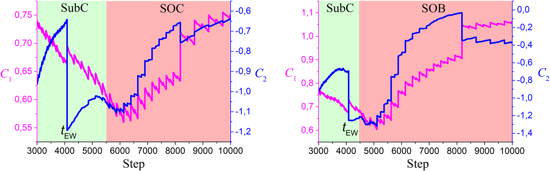
FIGURE 2. Time series of the log cumulants for the standard (left) and facilitated (right) BTW automaton.

All cellular automata show the same behavior $c_{1t}$ and $c_{2t}$, when approaching to $t_{\text{EW}}$ (Figure 2). A decrease in the value of $c_{1t}$ by the value $\Delta c_1^{-}$ is observed, accompanied by a sharp increase by the value $\Delta c_1^{+}$. For example, for BTW-ST-SL automaton $\Delta c_1^{-}=0.0776$ and $\Delta c_1^{+}=0.0343$. An increase in the value of $c_{1t}$ by the value $\Delta c_2^{+}$ is observed, accompanied by a sharp decrease by the value $\Delta c_2^{-}$. For example, for BTW-ST-SL automaton $\Delta c_2^{+}=0.2935$ and $\Delta c_2^{-}=0.5586$. Consequently, the approach to $t_{\text{EW}}$ is accompanied by an increase in the width of the singularity spectrum, and only at time $t_{\text{EW}}$ a sharp decrease in the spectrum occurs. The considered values $\Delta c$ are presented in Supplementary Table S2 for all cellular automata. In general, the behavior of the log cumulants is independent of the structure and rules of the automata.

Discussion

This Section presents a discussion of linking of our research results to some recent results from the theory of early warning indicators for critical transitions. Also, a discussion of possible practical applications of proposed early warning measures for detection of critical transitions is presented.

We will start by considering the main similarities and differences in the stochastic dynamics of the number of unstable cells $\left(x_t\right)$ of automata located in the SubC phase and in one of the critical states (the SOC state and the SOB state), summarizing the discussions from Result and Their Discussion. Common to automata with standard and facilitated rules is the multifractal structure $x_t$ in the SubC phase, and the monofractal (more precisely, a weak multifractal) structure $x_t$ in the SOC state (for the standard models) and in the SOB state (for the facilitated models). Such a transition into the critical state corresponds to the multifractal-monofractal transition (see the paper [33]). Another common feature is the long-range dependence (LRD) in the time series $\left(c_1>0.5\right)$ for cellular automata in the SubC phase. Therefore, this multifractality is due to the existence of long-term correlations of small and large fluctuations [34]. The only fundamental difference between the SOC state and the SOB state is the presence of the short-range dependence (SRD) in the $x_t$ in the first case $\left(c_1<0.5\right)$, and the presence of the LRD in the $x_t$ in the second case.

As it is shown in the paper [35], the average magnetization time series in the Ising model are multifractal in the SubC phase and in the critical state. Moreover, the structure of the time series is more heterogeneous in the critical state, than in the SubC phase. The increase of the memory in time series as the system approaches the critical point is also shown. In our opinion, a significant difference between the indicated results and those obtained by us lies in the fundamental difference between the rules for the Ising model and the rules for the sandpile cellular automata. In the paper [36], the results of the study of changes in the temporal autocorrelation at lag 1 and the power spectral density (PSD) as the system approaches to the critical point are presented. There was a significant increase in the autocorrelation in the neighborhood of the critical point, which is associated with the critical slowing down, as well as an increase in the parameter $\beta$ of the power law for PSD $\left(S\left(\omega \right)\propto {\omega }^{-\beta }\right)$. These results are consistent with our results for the facilitated model. Similar results are presented in [37–39], but obtained using fractal analysis methods. The results we obtained for facilitated models are also fully confirmed by the results presented in the papers [40–43]. However, the results similar to the one obtained by us for the standard models have not been presented yet.

The time series generated by real systems have a more complex structure than the time series generated by the sandpile cellular automata. However, we believe that the main features of $c_{1t}$ and $c_{2t}$ behavior, when the automata approach the critical state, will also be observed for real complex systems (see the papers [44, 45]). Let us take social media as an example. Recent studies have shown that most social networks are capable to self-organize into the critical state (see the papers [7, 46–51]). The mechanisms (local rules) for online social networks (for example, Twitter) for transition into the SOC state are similar to the standard rules of the sandpile cellular automaton on the BA graph. It is known (see the paper [52]) that the graph structure of user interactions in online social networks corresponds to BA graphs. Indeed, the information distribution is carried out by users who are in the state of high-level reflection (unstable state). It manifests itself in the form of reposts to their subscribers (neighboring nodes of the graph). These subscribers, being in the unstable state, send reposts to their subscribers, etc. As a result, starting from the moment $t_{\text{C}}$ avalanche-like distribution of information in the network is observed. On the contrary, the SubC phase ($t\in \left[0,t_{\text{C}}\right]$) of the online social network is characterized by stochastic fluctuations in repost activity with a relatively small amplitude. In most of such situations, it becomes necessary to evaluate $t_{\text{EW}}$, which is of undoubted interest for all specialists in social networks monitoring. Obtaining of such estimates for real time series of retweets relevant to various topics is one of the goals of our further studies.

Finally, we look at the limitations and possible further research in the analysis of critical transition precursors in sandy cellular automata.

We have established only one limitation of the proposed approach associated with the length of the analyzed time series and the large number of zero values in it. To obtain reliable results, the length of the time series must be at least 2000 steps. Otherwise, significant fluctuations in the value of the log cumulants are observed, in which it is impossible to determine their smoothed behavior.

From the point of view of the prospects for further research, in our opinion, one should focus on the interpretation of jumps in the values ​​of log-cumulants, which are characteristic of critical states of all cellular automata. An explanation of this empirical phenomenon is possible by analyzing the time series obtained under various initial conditions and sizes of all investigated cellular automata.

Data Availability Statement

The raw data supporting the conclusions of this article will be made available by the authors, without undue reservation.

Author Contributions

AD, VK, and VD designed the research. VK, VD and NA performed the simulations. NA prepared the figures. All authors contributed to writing and reviewing the manuscript.

Funding

The work is an output of a research project implemented as part of the Basic Research Program at the National Research University Higher School of Economics (HSE University).

Conflict of Interest

The authors declare that the research was conducted in the absence of any commercial or financial relationships that could be construed as a potential conflict of interest.

Publisher’s Note

All claims expressed in this article are solely those of the authors and do not necessarily represent those of their affiliated organizations, or those of the publisher, the editors, and the reviewers. Any product that may be evaluated in this article, or claim that may be made by its manufacturer, is not guaranteed or endorsed by the publisher.

Supplementary Material

The Supplementary Material for this article can be found online at: https://www.frontiersin.org/articles/10.3389/fphy.2022.839383/full#supplementary-material

References

1. Scheffer M, Carpenter SR, Lenton TM, Bascompte J, Brock W, Dakos V, et al. Anticipating Critical Transitions. Science (2012) 338:344–8. doi:10.1126/science.1225244

PubMed Abstract | CrossRef Full Text | Google Scholar

2. Morales IO, Landa E, Angeles CC, Toledo JC, Rivera AL, Temis JM, et al. Behavior of Early Warnings Near the Critical Temperature in the Two-Dimensional Ising Model. PLoS ONE (2015) 10:e0130751. doi:10.1371/journal.pone.0130751

PubMed Abstract | CrossRef Full Text | Google Scholar

3. Suweis S, D'Odorico P Early Warning Signs in Social-Ecological Networks. PLoS ONE (2014) 9:e101851. doi:10.1371/journal.pone.0101851

PubMed Abstract | CrossRef Full Text | Google Scholar

4. Scheffer M, Bascompte J, Brock WA, Brovkin V, Carpenter SR, Dakos V, et al. Early-warning Signals for Critical Transitions. Nature (2009) 461:53–9. doi:10.1038/nature08227

PubMed Abstract | CrossRef Full Text | Google Scholar

5. Dakos V, Carpenter SR, van Nes EH, Scheffer M Resilience Indicators: Prospects and Limitations for Early Warnings of Regime Shifts. Phil Trans R Soc B (2015) 370:20130263. doi:10.1098/rstb.2013.0263

CrossRef Full Text | Google Scholar

6. George SV, Kachhara S, Misra R, Ambika G Early Warning Signals Indicate a Critical Transition in Betelgeuse. A&A (2020) 640:L21. doi:10.1051/0004-6361/202038785

CrossRef Full Text | Google Scholar

7. Tadić B, Melnik R Self-Organised Critical Dynamics as a Key to Fundamental Features of Complexity in Physical, Biological, and Social Networks. Dynamics (2021) 1:181–97. doi:10.3390/dynamics1020011

CrossRef Full Text | Google Scholar

8. Bak P, Tang C, Wiesenfeld K Self-organized Criticality: An Explanation of the 1/fnoise. Phys Rev Lett (1987) 59:381–4. doi:10.1103/PhysRevLett.59.381

PubMed Abstract | CrossRef Full Text | Google Scholar

9. Shapoval A, Shapoval B, Shnirman M 1/x Power-Law in a Close Proximity of the Bak-Tang-Wiesenfeld Sandpile. Sci Rep (2021) 11:18151. doi:10.1038/s41598-021-97592-x

PubMed Abstract | CrossRef Full Text | Google Scholar

10. Buendía V, di Santo S, Bonachela JA, Muñoz MA Feedback Mechanisms for Self-Organization to the Edge of a Phase Transition. Front Phys (2020) 8:333. doi:10.3389/fphy.2020.00333

CrossRef Full Text | Google Scholar

11. Cocchi L, Gollo LL, Zalesky A, Breakspear M Criticality in the Brain: A Synthesis of Neurobiology, Models and Cognition. Prog Neurobiol (2017) 158:132–52. doi:10.1016/j.pneurobio.2017.07.002

PubMed Abstract | CrossRef Full Text | Google Scholar

12. Buendía V, di Santo S, Villegas P, Burioni R, Muñoz MA Self-organized Bistability and its Possible Relevance for Brain Dynamics. Phys Rev Res (2020) 2:013318. doi:10.1103/PhysRevResearch.2.013318

CrossRef Full Text | Google Scholar

13. di Santo S, Burioni R, Vezzani A, Muñoz MA Self-organized Bistability Associated with First-Order Phase Transitions. Phys Rev Lett (2016) 116:240601. doi:10.1103/PhysRevLett.116.240601

PubMed Abstract | CrossRef Full Text | Google Scholar

14. Járai AA The Sandpile Cellular Automaton. In: Louis PY, and Nardi F, editors. Probabilistic Cellular Automata. Emergence, Complexity and Computation, Vol. 27 (2018). p. 79–88. doi:10.1007/978-3-319-65558-1_6

CrossRef Full Text | Google Scholar

15. Bak P, Tang C, Wiesenfeld K Self-organized Criticality. Phys Rev A (1988) 38:364–74. doi:10.1103/PhysRevA.38.364

CrossRef Full Text | Google Scholar

16. Feder HJS, Feder J Self-organized Criticality in a Stick-Slip Process. Phys Rev Lett (1991) 66:2669–72. doi:10.1103/PhysRevLett.66.2669

PubMed Abstract | CrossRef Full Text | Google Scholar

17. Manna SS Two-state Model of Self-Organized Criticality. J Phys A: Math Gen (1991) 24:L363–L369. doi:10.1088/0305-4470/24/7/009

CrossRef Full Text | Google Scholar

18. Albert R, Barabási A-L Statistical Mechanics of Complex Networks. Rev Mod Phys (2002) 74:47–97. doi:10.1103/RevModPhys.74.47

CrossRef Full Text | Google Scholar

19. Newman MEJ, Strogatz SH, Watts DJ Random Graphs with Arbitrary Degree Distributions and Their Applications. Phys Rev E (2001) 64:026118. doi:10.1103/PhysRevE.64.026118

CrossRef Full Text | Google Scholar

20. Buldyrev SV, Parshani R, Paul G, Stanley HE, Havlin S Catastrophic cascade of Failures in Interdependent Networks. Nature (2010) 464:1025–8. doi:10.1038/nature08932

PubMed Abstract | CrossRef Full Text | Google Scholar

21. Cannings C, Penman DB Ch. 2. Models of Random Graphs and Their Applications. Handbook Stat (2003) 21:51–91. doi:10.1016/S0169-7161(03)21004-X

CrossRef Full Text | Google Scholar

22. Arneodo A, Bacry E, Muzy JF The Thermodynamics of Fractals Revisited with Wavelets. Physica A: Stat Mech its Appl (1995) 213:232–75. doi:10.1016/0378-4371(94)00163-N

CrossRef Full Text | Google Scholar

23. Muzy JF, Bacry E, Arneodo A Multifractal Formalism for Fractal Signals: The Structure-Function Approach versus the Wavelet-Transform Modulus-Maxima Method. Phys Rev E (1993) 47:875–84. doi:10.1103/PhysRevE.47.875

CrossRef Full Text | Google Scholar

24. Yamamoto M. Fluctuations Observed in Biological Time Series Signals and Their Functional Significance. Front Med Biol Eng (1991) 3:135–7.

PubMed Abstract | Google Scholar

25. Ihlen EAF Introduction to Multifractal Detrended Fluctuation Analysis in Matlab. Front Physio (2012) 3:141. doi:10.3389/fphys.2012.00141

CrossRef Full Text | Google Scholar

26. Kantelhardt JW, Zschiegner SA, Koscielny-Bunde E, Havlin S, Bunde A, Stanley HE Multifractal Detrended Fluctuation Analysis of Nonstationary Time Series. Physica A: Stat Mech its Appl (2002) 316:87–114. doi:10.1016/S0378-4371(02)01383-3

CrossRef Full Text | Google Scholar

27. Mallat S, Hwang WL Singularity Detection and Processing with Wavelets. IEEE Trans Inform Theor (1992) 38:617–43. doi:10.1109/18.119727

CrossRef Full Text | Google Scholar

28. Wendt H, Abry P Multifractality Tests Using Bootstrapped Wavelet Leaders. IEEE Trans Signal Process (2007) 55:4811–20. doi:10.1109/TSP.2007.896269

CrossRef Full Text | Google Scholar

29. Jaffard S, Lashermes B, Abry P Wavelet Leaders in Multifractal Analysis. In: Qian T, Vai MI, and Yuesheng X, editors. Wavelet Analysis and Applications (2006). p. 201–46. doi:10.1007/978-3-7643-7778-6_17

CrossRef Full Text | Google Scholar

30. Wendt H, Roux SG, Abry P Bootstrap for Log Wavelet Leaders Cumulant Based Multifractal Analysis. In: 2006 14th European Signal Processing Conference (2006). p. 1–5.

Google Scholar

31. Ciuciu P, Abry P, Rabrait C, Wendt H Log Wavelet Leaders Cumulant Based Multifractal Analysis of EVI fMRI Time Series: Evidence of Scaling in Ongoing and Evoked Brain Activity. IEEE J Sel Top Signal Process (2008) 2:929–43. doi:10.1109/JSTSP.2008.2006663

CrossRef Full Text | Google Scholar

32. Wendt H Contributions of Wavelet Leaders and Bootstrap to Multifractal Analysis: Images, Estimation Performance, Dependence Structure and Vanishing Moments. Confidence Intervals and Hypothesis Tests. Signal and Image Processing. Lyon, France: Ecole normale superieure de lyon - ENS LYON (2008). Available from: https://tel.archives-ouvertes.fr/tel-00333599/document (Accessed December 5, 2021).

Google Scholar

33. Murcio R, Masucci AP, Arcaute E, Batty M Multifractal to Monofractal Evolution of the London Street Network. Phys Rev E (2015) 92. doi:10.1103/PhysRevE.92.062130

CrossRef Full Text | Google Scholar

34. Zhou W-X Finite-size Effect and the Components of Multifractality in Financial Volatility. Chaos, Solitons & Fractals (2012) 45:147–55. doi:10.1016/j.chaos.2011.11.004

CrossRef Full Text | Google Scholar

35. Zhao L, Li W, Yang C, Han J, Su Z, Zou Y Multifractality and Network Analysis of Phase Transition. PLoS ONE (2017) 12:e0170467. doi:10.1371/journal.pone.0170467

PubMed Abstract | CrossRef Full Text | Google Scholar

36. Morales IO, Landa E, Angeles CC, Toledo JC, Rivera AL, Temis JM, et al. Behavior of Early Warnings Near the Critical Temperature in the Two-Dimensional Ising Model. PLoS ONE (2015) 10:e0130751. doi:10.1371/journal.pone.0130751

PubMed Abstract | CrossRef Full Text | Google Scholar

37. Rypdal M Early-Warning Signals for the Onsets of Greenland Interstadials and the Younger Dryas-Preboreal Transition. J Clim (2016) 29:4047–56. doi:10.1175/JCLI-D-15-0828.1

CrossRef Full Text | Google Scholar

38. Zhang X, Xu Y, Liu Q, Kurths J, Grebogi C Rate-dependent Tipping and Early Warning in a Thermoacoustic System under Extreme Operating Environment. Chaos (2021) 31:113115. doi:10.1063/5.0071977

PubMed Abstract | CrossRef Full Text | Google Scholar

39. Dexing L, Enyuan W, Xiangguo K, Xiaoran W, Chong Z, Haishan J, et al. Fractal Characteristics of Acoustic Emissions from Coal under Multi-Stage True-Triaxial Compression. J Geophys Eng (2018) 15:2021–32. doi:10.1088/1742-2140/aac31a

CrossRef Full Text | Google Scholar

40. Dakos V, Carpenter SR, Brock WA, Ellison AM, Guttal V, Ives AR, et al. Methods for Detecting Early Warnings of Critical Transitions in Time Series Illustrated Using Simulated Ecological Data. PLoS ONE (2012) 7:e41010. doi:10.1371/journal.pone.0041010

PubMed Abstract | CrossRef Full Text | Google Scholar

41. van der Bolt B, van Nes EH, Scheffer M No Warning for Slow Transitions. J R Soc Interf (2021) 18:20200935. doi:10.1098/rsif.2020.0935

CrossRef Full Text | Google Scholar

42. Diks C, Hommes C, Wang J Critical Slowing Down as an Early Warning Signal for Financial Crises? Empir Econ (2019) 57:1201–28. doi:10.1007/s00181-018-1527-3

CrossRef Full Text | Google Scholar

43. Zhang Z, Li Y, Hu L, Tang Ca., Zheng H Predicting Rock Failure with the Critical Slowing Down Theory. Eng Geology (2021) 280:105960. doi:10.1016/j.enggeo.2020.105960

CrossRef Full Text | Google Scholar

44. Aschwanden MJ, Crosby NB, Dimitropoulou M, Georgoulis MK, Hergarten S, McAteer J, et al. 25 Years of Self-Organized Criticality: Solar and Astrophysics. Space Sci Rev (2016) 198:47–166. doi:10.1007/s11214-014-0054-6

CrossRef Full Text | Google Scholar

45. Lise S, Paczuski M Self-organized Criticality and Universality in a Nonconservative Earthquake Model. Phys Rev E (2001) 63:036111. doi:10.1103/PhysRevE.63.036111

CrossRef Full Text | Google Scholar

46. Zhukov D, Kunavin K, Lyamin S Online Rebellion: Self-Organized Criticality of Contemporary Protest Movements. SAGE Open (2020) 10:215824402092335. doi:10.1177/2158244020923354

CrossRef Full Text | Google Scholar

47. Tadic B Self-organised Criticality and Emergent Hyperbolic Networks: Blueprint for Complexity in Social Dynamics. Eur J Phys (2019) 40:024002. doi:10.1088/1361-6404/aaf144/meta

CrossRef Full Text | Google Scholar

48. Dmitriev A, Dmitriev V Identification of Self-Organized Critical State on Twitter Based on the Retweets' Time Series Analysis. Complexity (2021) 2021:6612785. doi:10.1155/2021/6612785

CrossRef Full Text | Google Scholar

49. Dmitriev A, Dmitriev V, Balybin S Self-Organized Criticality on Twitter: Phenomenological Theory and Empirical Investigation Based on Data Analysis Results. Complexity (2019) 2019:8750643. doi:10.1155/2019/8750643

CrossRef Full Text | Google Scholar

50. Wang Y, Fan H, Lin W, Lai Y-C, Wang X Growth, Collapse and Self-Organized Criticality in Complex Networks. Sci Rep (2016) 6:24445. doi:10.1038/srep24445

PubMed Abstract | CrossRef Full Text | Google Scholar

51. Tadić B, Dankulov MM, Melnik R Mechanisms of Self-Organized Criticality in Social Processes of Knowledge Creation. Phys Rev E (2017) 96:032307. doi:10.1103/PhysRevE.96.032307

PubMed Abstract | CrossRef Full Text | Google Scholar

52. Broido AD, Clauset A Scale-free Networks Are Rare. Nat Commun (2019) 10:1017. doi:10.1038/s41467-019-08746-5

PubMed Abstract | CrossRef Full Text | Google Scholar