Simulating the Responses of the Magnetosphere–Ionosphere System to the IMF By Reversal

Introduction

The solar wind-magnetosphere interaction is largely controlled by the interplanetary magnetic field (IMF). Various investigations investigated the magnetosphere-ionosphere (MI) response to sudden changes in the IMF based on observations and numerical simulations (e.g., [1–9]). For example, Wing et al. [10] reported that following a sudden orientation change of the IMF B_z, the geomagnetic field on the dayside of geosynchronous orbit responds in 4–5 min while that on the nightside reacts in 12 min. Yu and Ridley [11] simulated the magnetosphere-ionosphere responses to a sudden southward turning of the IMF B_z component and found that, depending on the solar wind speed, the ionospheric convection responds in 4–8 min and the magnetosphere reconfigures into a new state within 15–20 min.

On the other hand, the IMF B_y plays an important role in modifying the magnetospheric configuration and introducing asymmetric magnetic flux across two hemispheres. With the presence of duskward IMF B_y, the dayside magnetopause reconnection shifts to the northern duskward and southern dawnward quadrants. Such a dawn-dusk asymmetry introduces asymmetric magnetic flux onto the tail magnetosphere, resulting in the appearance of the y-component of the geomagnetic field in the magnetotail, or called IMF B_y penetration. According to 9 years of cluster observations, Cao et al. [12] found that the neutral sheet B_y is nearly linearly correlated to the IMF B_y, and the penetration efficiency of the IMF B_y is enhanced under southward IMF conditions. Browett et al. [13] further expanded the statistical work of Cao et al. [12]. They found that the response of plasma sheet to IMF B_y in the case of southward IMF is obviously faster than that of northward IMF. However, the time delay in responding to sudden IMF B_y variations was not considered in their statistical analysis. Rong et al. [14] reported a time delay of 1–1.5 h for the IMF B_y penetration into the magnetotail. But Kabin et al. [15] found the response time scale to be 4–8 min and 14–20 min in the dayside and nightside magnetosphere respectively. Tenfjord et al. [16] surveyed the Geostationary Operational Environmental Satellite (GOES) satellite observations and reported an average response time of about 15 min over all local times and a reconfiguration time of about 45 min at geosynchronous distances following the IMF B_y reversal.

Using idealized simulations, Tenfjord et al. [17] illustrated the magnetic induction process in the magnetosphere associated with the IMF B_y emergence. Their study assumed a gradual emergence of IMF B_y (within 10 min) from a purely northward IMF B_z condition instead of a sudden orientation change of IMF B_y. We speculate that a pre-existing y-component of the geomagnetic field effect probably would affect the response processes. Therefore, in this study, we simulate the MI system in response to an abrupt IMF B_y reversal (within 1 min) from duskward to dawnward, intending to reveal the transitional responses in both the ionosphere and the magnetotail in a global context. Such a sudden IMF B_y orientation change without varying other solar wind/IMF parameters indicates a tangential discontinuity. Our analysis of the magnetospheric configuration and ionospheric electrodynamics suggests that the ionosphere reacts in a few minutes but spends about 30 min finishing the transition, while the tail magnetosphere reconfigures in a much longer time. The magnetotail reconfiguration transits in a much slower and more complicated way under northward IMF conditions than under southward IMF conditions.

Methodology

We use the Space Weather Modeling Framework (SWMF) [18,19] to simulate the response of the MI system to the sudden orientation change of the IMF B_y. The SWMF contains the global MHD model BATS-R-US that solves the ideal MHD equations [20], and an ionospheric potential solver [21]. The electric potential is determined by ionospheric conductance and field-aligned currents (FACs), which are calculated at a sphere of 3.0 Earth radius (R_E) in the MHD model and mapped to the ionosphere altitude. The ionosphere conductance is specified based on two dominant sources: the solar EUV-generated conductance and the auroral zone conductance [21]. The resultant electric potential is mapped back to the inner boundary of the MHD model (i.e., 2.5 R_E) to determine the convection velocity. Such an integrated model is suitable for solving the geospace circulation dynamics and has been extensively validated (e.g., [22–27]).

The simulation is an idealized numerical experiment with the Earth’s rotation axis aligned with the magnetic dipole axis. The solar wind input of the model at the upstream boundary includes a simple step function of IMF B_y from 5 nT to −5 nT (i.e., from duskward to dawnward), with other solar wind parameters remaining constant: solar wind density n = 5/cm³, U_x = −400 km/s, U_y = U_z = 0, B_x = 0, B_z = 5nT, and T = 100,000K. The simulation is firstly run for 1 hour before IMF B_y is abruptly flipped, after which the simulation continues for 5 h.

Simulation Results

To understand how the global magnetosphere changes in response to the IMF B_y turning from duskward to dawnward, several snapshots of the global magnetic configuration are shown in Figure 1. It is found that after the IMF B_y reversal arrives at the bow shock (denoted as t = 0 min), the dawnward B_y gradually occupies the magnetosheath and then the cusp regions in both hemispheres from t = 9 to 28 min. Note that as the dawnward IMF B_y approaches the dayside magnetopause and the originally strong duskward B_y in the cusp region gradually decreases (red turning to green), the nightside magnetospheric configuration is hardly affected until t = 28 min, after which the duskward y-component of the geomagnetic field in the magnetotail neutral sheet starts fading. However, an enhancement of the duskward geomagnetic field appears again at t = 34 min around X ∼ −18 R_E and propagates Earthward. This is due to a temporary twist of magnetic fields in the near-Earth region, as will be discussed later. After t = 54 min, the dawnward geomagnetic field starts to emerge in the far magnetotail at X ∼ −40 R_E and moves Earthward, while in the middle-tail region around −20 R_E < X < −10 R_E, the duskward geomagnetic field remains and continues decreasing. The far-tail dawnward geomagnetic field penetrates Earthward and the global configuration finally stabilizes after ∼2 h.

FIGURE 1

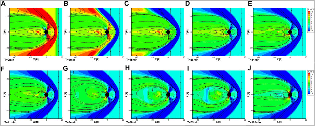
FIGURE 1. Global magnetospheric configuration in the XZ plane. Color indicates B_y component. The black streamlines represent magnetic field lines.

It demonstrates that the dayside ionosphere is influenced much earlier than the nightside magnetosphere due to the direct penetration of IMF B_y into the high-latitude cusp region, and the nightside magnetosphere does not seem to react linearly with radial distance. We therefore investigate the ionosphere and nightside magnetosphere separately in detail. Figure 2 shows the evolution of the FACs pattern in the northern hemisphere. The initial NBZ current consists of a bulk upward (red) current in the polar cap region and an elongated downward (blue) current at 75° magnetic latitude in the dawn sector. After the reversed IMF B_y encountering the high-latitude lobe reconnection site (as seen in Figure 1) at t = 9 min, a new upward FACs in the post-noon sector at 75° magnetic latitude starts to grow, while the original NBZ current system fades (from t = 9 min to t = 30 min). The growth of the new upward FACs into an elongated pattern in the dusk sector is accompanied by downward FACs at an even higher latitude in the post-noon, which eventually becomes a bulk current. The new state, established after about 40 min, is an expected pattern with the opposite IMF B_y orientation. We note that the ionospheric FACs do not respond until about 10 min after the IMF B_y reversal arrives at the bow shock. Such a belated effect is owing to the transitional development of the new reconnection site in the dawn sector, rather than an instantaneous shift from dusk to dawn.

FIGURE 2

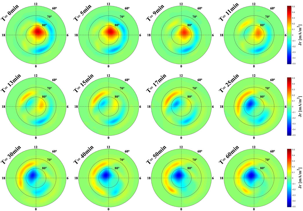
FIGURE 2. Ionospheric FACs pattern in the northern hemisphere. Red indicates upward current and blue indicates downward current.

Figure 3 shows the change of magnetic topology at X = −1 R_E. The chosen position is based on the location of lobe reconnection. All the field lines are projected to the YZ plane. Colors on field lines indicate By. The contour colors denote E•J, an indicator of energy conversion. A negative value suggests energy conversion from plasma kinetic energy to electromagnetic energy, and a positive value means the opposite conversion. The outer-most purple circle denotes the bow shock, and the internal circle represents the magnetopause boundary. Initially, the duskward IMF B_y (red) is reconnected with the geomagnetic field in the duskside lobe at t = 0 min. One of the reconnected field lines is open and connected to the southern polar region, while the other one is connected to the northern cap and open to the northern hemisphere. A similar reconnection occurs in the southern hemisphere in the dawnside lobe. The arrival of dawnward IMF B_y (blue) in the magnetosheath at t = 5 min only changes the orientation of the originally connected field lines outside the magnetopause, forming a “Z”-shaped reconnected field line still connecting to the other hemisphere. This “Z”-shaped line relaxes into a more stretched line at t = 9 min, with the reconnection site moving to the midnight meridian. Two minutes later, the stretched dawnward IMF line is reconnected again at the high latitude lobe region. This time it is near the midnight meridian local time toward dawn. The new reconnection brings in new energy sources down to the high-latitude polar region to generate the new FAC pattern. Such a dynamic evolution of the newly approaching IMF B_y from the dayside magnetosheath to the new high-latitude nightside lobe leads to a delayed reaction in the ionosphere by ∼10 min. Later on, the new reconnection site migrates dawnward while keeping the topology unchanged.

FIGURE 3

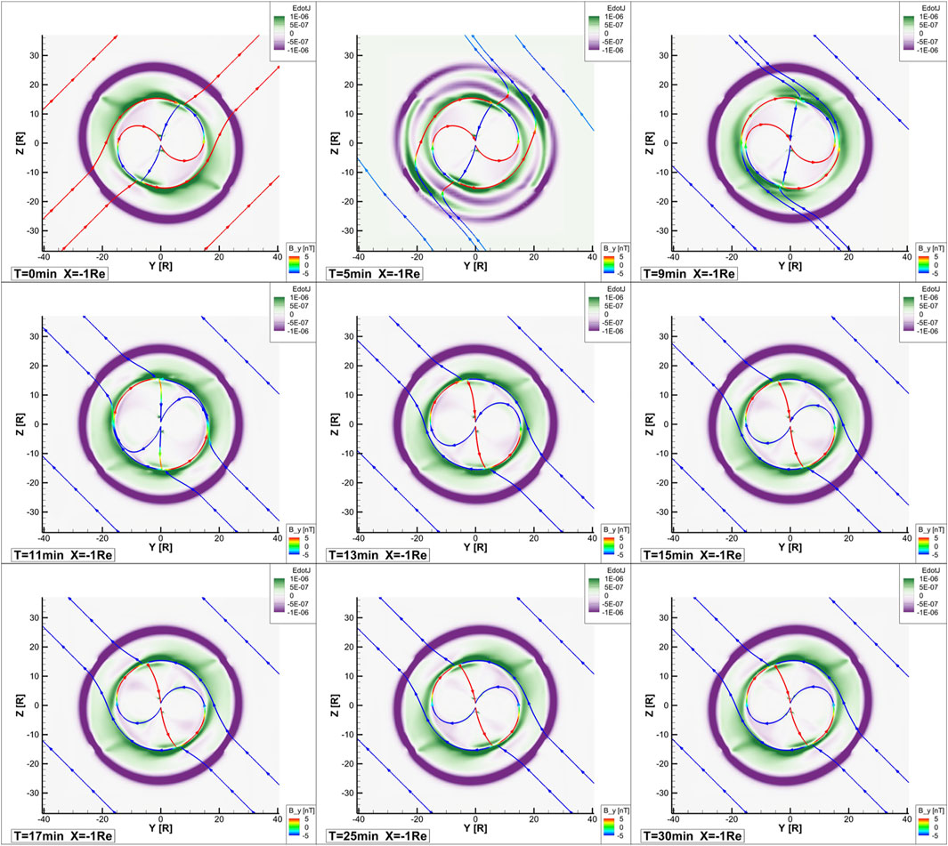
FIGURE 3. Magnetic field lines projected to the YZ plane at X = −1 R_E. The color on the lines indicates B_y. The contour color in the background represents E•J.

Figure 4 shows the temporal evolution of the 3D magnetotail configuration, to understand the response in the nightside magnetosphere. Field lines are selected with their footprints fixed in the ionosphere throughout the process. Colors on the field lines denote the y-component of the geomagnetic field. Initially, with IMF B_y>0, the middle-tail field lines (X∼−10 R_E) are twisted with a moderate duskward geomagnetic field in the neutral sheet (shown in yellow), while the far-tail region (X ∼ −30 R_E) is less twisted. Such a configuration does not change much until approximately 30 min after the bow shock encounter of the IMF B_y reversal. At t = 36 min, the near-Earth y-component of the geomagnetic field in the neutral sheet is significantly enhanced as the magnetic field lines are pushed to be highly duskward (large positive B_y in red), likely a result of Earthward depolarization and bursty flows. The field line stretching and depolarization can be seen in Figure 1 at t = 34 and 41 min. The contour color of U_x in the magnetic equator suggests a fast Earthward flow. Calculation of E•J (not shown) also indicates an energy transfer from electromagnetic energy to kinetic energy, i.e., an indication of local reconnection. As the highly twisted duskward magnetic field lines in the neutral sheet gradually relax, the off-equator magnetic field starts to change to dawnward (see t = 40 min). After t = 60 min, the tail magnetic fields clearly show dawnward tilt, although the middle-tail fields still appear to be aligned with the midnight meridian with very limited tilt in the Y direction.

FIGURE 4

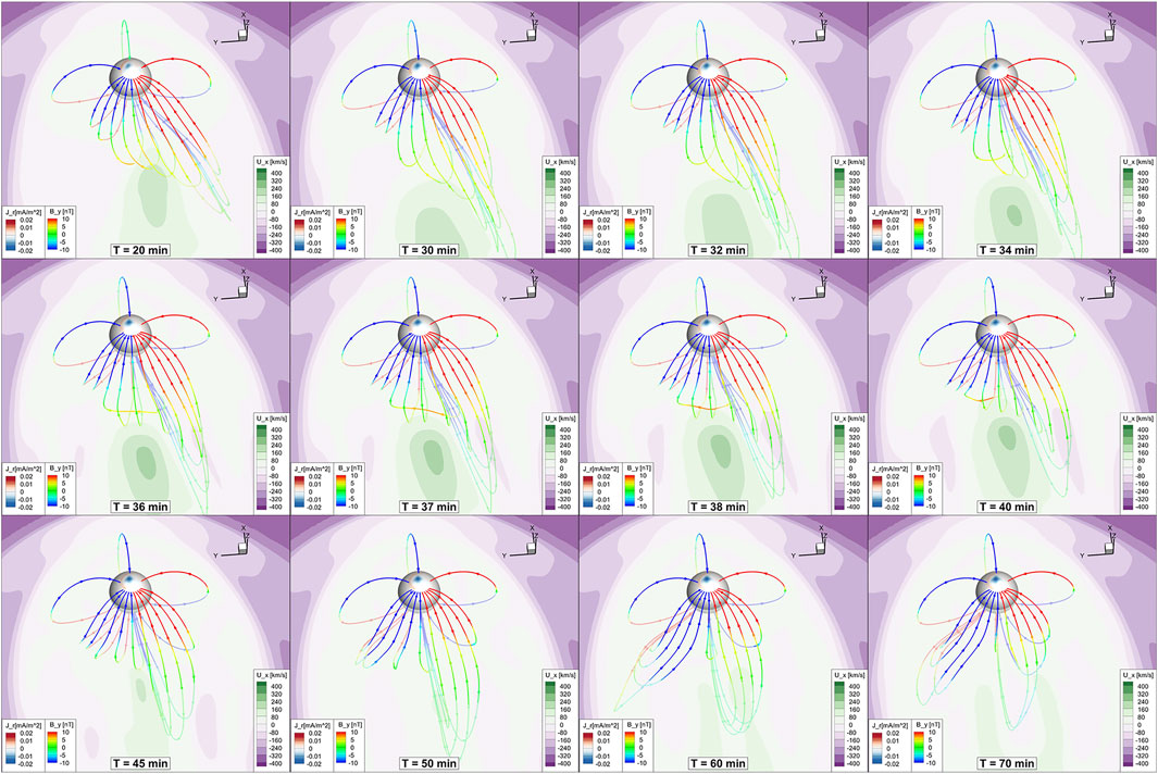
FIGURE 4. Nightside magnetospheric configuration. Streamlines indicate magnetic field lines with the color representing B_y component. The background color indicates U_x. The color on the sphere near the Earth indicates FACs (Jr).

Discussion

The above simulation reveals the MI response to the IMF B_y reversal (from duskward to dawnward) under northward IMF conditions. It is found that the ionosphere can quickly react within 10 min, although the entire reconfiguration to the new FACs pattern takes about another 30 min. On the other hand, the magnetotail reconfiguration is more complex. The near-Earth duskward geomagnetic field undergoes an enhancement before the dawnward geomagnetic field is finally induced. The middle-tail geomagnetic field does not change much even after t = 60 min. Whether a similar reconfiguration process takes place if the IMF B_z<0 is not well known. Therefore, a new simulation with the IMF B_z = −5 nT has been carried out. It is found that the ionospheric responses are similar. That is, after the arrival of the IMF B_y reversal on the magnetopause, the FACs start to react within 10 min and gradually shift to a new state. But the magnetotail fields appear to respond in a much simpler way.

Figure 5 shows the response time of the y-component of geomagnetic fields at any location in the central plasma sheet along the Sun-Earth line. The time of zero is defined when the IMF By discontinuity encounters the bow shock, and the response time at a location along the Sun-Earth line is recorded when the geomagnetic field changes from duskward to dawnward. The black dashed line marks the propagating time of the IMF By discontinuity. In general, the y-component of the geomagnetic field responds in a faster way under IMF B_z < 0 than under IMF B_z > 0. While the response time in the dayside magnetosphere in both cases monotonically increases with decreasing distances, the nightside magnetosphere shows vastly different response times. With IMF B_z < 0, the near-Earth region (X > −13 R_E) reacts quickly within 10–30 min, depending on the distance from the Earth. Around X ∼ −13 R_E, an abrupt change in response time denotes the tail reconnection site, beyond which the reconnected magnetic fields are completely open in the solar wind and need 40 min to respond, without a clear distance-dependence though. In contrast, with IMF B_z > 0, the near-Earth and far-tail regions can quickly react with a time scale of 20–60 min. Note that the signal of duskward-to-dawnward turning of magnetic fields in these two regions appears to propagate in opposite directions, both towards the middle-tail region, which ends up with a very late response. After analyzing the 3D configuration, it is found that the field lines in the middle-tail region are firstly twisted more duskward and then slowly recover and stay aligned with the midnight meridian for a while before they finally turn dawnward. Such a reluctant response may be associated with shear flows in the azimuthal direction, which helps balance the forces from the twisted magnetic field. Figure 6 displays the field configuration with the flow speed shown in color. At t = 70 min, a fast Earthward flow from the tail diverges to east/west directions near X ∼ −15 R_E, and remains at a high speed of ∼100 km/s. This strong shear flow lasts for about 20 min before disappearing. This is consistent with the response time in the middle-tail region. Therefore, the slow response in the middle-tail region is probably hindered by the external forces in association with fast shear flows.

FIGURE 5

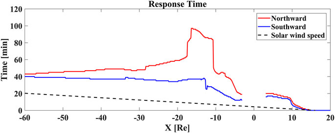
FIGURE 5. Response time of the y-component of the geomagnetic field variation on the Sun-Earth line under northward (red) and southward (blue) IMF B_z conditions.

FIGURE 6

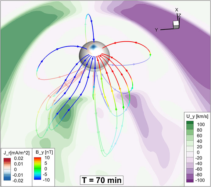
FIGURE 6. Magnetic configuration at t = 70 min with the equatorial flow speed indicated by color.

We speculate that the difference between the two cases is ultimately due to different magnetic flux loading processes from the dayside reconnection. As the magnetosphere is open under IMF B_z < 0 due to both the dayside and nightside magnetic reconnection, the asymmetric magnetic flux from the dayside magnetopause can be easily exerted on the nightside lobe magnetosphere and then the tail reconnection through the Dungey cycle. On the other hand, when IMF B_z > 0, the magnetosphere is closed in a vast region even down to X < −60 R_E, and the reconnection occurs only in high-latitude tail lobes. Therefore, the asymmetric magnetic flux from the lobe reconnection cannot directly penetrate the middle-tail magnetosphere without the assistance of tail reconnection, but rather introduce disturbances on the magnetopause first and later induces the dawnward geomagnetic field through it. This also explains the longer time scales. Exactly through what kind of mechanism requires further investigation and we plan to do it in our future study.

Summary

IMF B_y is one of the most critical conditions that control the electromagnetic energy input into the MI system, leading to asymmetric responses in the system. In this study, we analyzed the transitional responses in the ionospheric FACs and magnetospheric configuration after the IMF B_y suddenly changing its orientation using MHD simulations. We mainly focused on solar wind conditions with the northward IMF B_z. The main results are summarized as follows.

1) The ionospheric FACs pattern responds in about 10 min after the IMF B_y discontinuity encounters the bow shock. The delayed response is because of the propagation of reversed IMF B_y inside the magnetosheath before touching the high-latitude lobe reconnection. Later on, the gradual reconfiguration of the reconnected field lines in the high-latitude lobes from dusk to the dawn sector takes another 5 min, and the penetration of reversed B_y into the cusp region is not significant until about 15 min later. Thus, the ionosphere reconfiguration needs about 30 min at least. This is consistent with the result of Kabin et al. [15].

2) In contrast to the quick response in the ionosphere, the magnetospheric response time on the nightside is longer. The local y-component of the geomagnetic field in the nightside neutral sheet does not change much until approximately 30 min later after the arrival of the IMF B_y turning signal at the bow shock. It is consistent with the result in Tenfjord et al. [17] that the response time is about 30 min based on an observational study of Geostationary Operational Environmental Satellite (GOES) data. However, the response time is not linearly correlated with the radial distance. Instead, the near-Earth (X > −15 R_E) and far-tail (X < −30 R_E) regions appear to have a quicker reaction with a time scale of 20–60 min than the middle-tail zone (−30 R_E < X < −15 R_E), which responds in about 80–100 min. The slow response in the middle-tail is probably due to local disturbances, such as localized dipolarization and flow burst.

3) The response is less complex when IMF B_z < 0. The response time scales throughout the magnetosphere are shorter than when IMF B_z > 0, consistent with the observational results in Browett et al. [13]. The response time also shows a linear correlation with the radial distance inside the closed field line region. The above mentioned comparison suggests that the asymmetric magnetic flux loading from the dayside reconnection site to the nightside magnetosphere may differ. As IMF B_z < 0, the loading can directly occur via the open tail reconnection, while this is not easy when the magnetosphere is largely closed if IMB B_z > 0.

Data Availability Statement

The raw data supporting the conclusions of this article will be made available by the authors, without undue reservation.

Author Contributions

FG performed the simulations, analyzed and visualized the results, and wrote the draft manuscript. YY provided the project idea, helped with the result interpretation, and revised the manuscript. JC contributed comments and edits to the manuscript.

Funding

This work is supported by NSFC grant 41821003.

Conflict of Interest

The authors declare that the research was conducted in the absence of any commercial or financial relationships that could be construed as a potential conflict of interest.

Publisher’s Note

All claims expressed in this article are solely those of the authors and do not necessarily represent those of their affiliated organizations, or those of the publisher, the editors, and the reviewers. Any product that may be evaluated in this article, or claim that may be made by its manufacturer, is not guaranteed or endorsed by the publisher.

Acknowledgments

This work was carried out using the SWMF and BATS-R-US tools developed at the University of Michigan’s Center for Space Environment Modeling (CSEM). Simulations were performed on the Tianhe-2 National Supercomputer Center in Guangzhou, China.

References

1. Nishida A. Coherence of geomagneticDP2 Fluctuations with Interplanetary Magnetic Variations. J Geophys Res (1968) 73(17):5549–59. doi:10.1029/JA073i017p05549

CrossRef Full Text | Google Scholar

2. Friis-Christensen E, Kamide Y, Richmond AD, Matsushita S. Interplanetary Magnetic Field Control of High-Latitude Electric fields and Currents Determined from Greenland Magnetometer Data. J Geophys Res (1985) 90(A2):1325–38. doi:10.1029/JA090iA02p01325

CrossRef Full Text | Google Scholar

3. Ridley AJ, Clauer CR. Characterization of the Dynamic Variations of the Dayside High-Latitude Ionospheric Convection Reversal Boundary and Relationship to Interplanetary Magnetic Field Orientation. J Geophys Res (1996) 101(A5):10919–38. doi:10.1029/JA101iA05p10919

CrossRef Full Text | Google Scholar

4. Dudeney JR, Rodger AS, Freeman MP, Pickett J, Scudder J, Sofko G, et al. The Nightside Ionospheric Response to IMF by Changes. Geophys Res Lett (1998) 25(14):2601–4. doi:10.1029/98GL01413

CrossRef Full Text | Google Scholar

5. Khan H, Cowley SWH. Observations of the Response Time of High-Latitude Ionospheric Convection to Variations in the Interplanetary Magnetic Field Using EISCAT and IMP-8 Data. Ann Geophys (1999) 17:1306–35. doi:10.1007/s00585-999-1306-8

CrossRef Full Text | Google Scholar

6. Lu G, Holzer TE, Lummerzheim D, Ruohoniemi JM, Stauning P, Troshichev O, et al. Ionospheric Response to the Interplanetary Magnetic Field Southward Turning: Fast Onset and Slow Reconfiguration. J Geophys Res (2002) 107(A8):2–1. doi:10.1029/2001JA000324

CrossRef Full Text | Google Scholar

7. Ruohoniemi JM, Shepherd SG, Greenwald RA. The Response of the High-Latitude Ionosphere to IMF Variations. J Atmos Solar-Terrestrial Phys (2002) 64(2):159–71. doi:10.1016/S1364-6826(01)00081-5

CrossRef Full Text | Google Scholar

8. Merkin VG, Anderson BJ, Lyon JG, Korth H, Wiltberger M, Motoba T. Global Evolution of Birkeland Currents on 10 Min Timescales: MHD Simulations and Observations. J Geophys Res Space Phys (2013) 118:4977–97. doi:10.1002/jgra.50466

CrossRef Full Text | Google Scholar

9. Tenfjord P, Østgaard N, Snekvik K, Laundal KM, Reistad JP, Haaland S, et al. How the IMF B Y Induces a B Y Component in the Closed Magnetosphere and How it Leads to Asymmetric Currents and Convection Patterns in the Two Hemispheres. J Geophys Res Space Phys (2015) 120:9368–84. doi:10.1002/2015JA021579

CrossRef Full Text | Google Scholar

10. Wing S, Sibeck DG, Wiltberger M, Singer H. Geosynchronous Magnetic Field Temporal Response to Solar Wind and IMF Variations. J Geophys Res (2002) 107(A8):32–1. doi:10.1029/2001JA009156

CrossRef Full Text | Google Scholar

11. Yu Y, Ridley AJ. Response of the Magnetosphere-Ionosphere System to a Sudden Southward Turning of Interplanetary Magnetic Field. J Geophys Res (2009) 114:n/a. doi:10.1029/2008JA013292

CrossRef Full Text | Google Scholar

12. Cao J, Duan A, Dunlop M, Wei X, Cai C. Dependence of IMFBypenetration into the Neutral Sheet on IMFBzand Geomagnetic Activity. J Geophys Res Space Phys (2014) 119:5279–85. doi:10.1002/2014JA019827

CrossRef Full Text | Google Scholar

13. Browett SD, Fear RC, Grocott A, Milan SE. Timescales for the Penetration of IMF B Y into the Earth's Magnetotail. J Geophys Res Space Phys (2017) 122:579–93. doi:10.1002/2016JA023198

CrossRef Full Text | Google Scholar

14. Rong ZJ, Lui ATY, Wan WX, Yang YY, Shen C, Petrukovich AA, et al. Time Delay of Interplanetary Magnetic Field Penetration into Earth's Magnetotail. J Geophys Res Space Phys (2015) 120:3406–14. doi:10.1002/2014JA020452

CrossRef Full Text | Google Scholar

15. Kabin K, Rankin R, Marchand R, Gombosi TI, Clauer CR, Ridley AJ, et al. Dynamic Response of Earth's Magnetosphere toByreversals. J Geophys Res (2003) 108:1132. doi:10.1029/2002JA009480

CrossRef Full Text | Google Scholar

16. Tenfjord P, Østgaard N, Strangeway R, Haaland S, Snekvik K, Laundal KM, et al. Magnetospheric Response and Reconfiguration Times Following IMF B Y Reversals. J Geophys Res Space Phys (2017) 122:417–31. doi:10.1002/2016JA023018

CrossRef Full Text | Google Scholar

17. Tenfjord P, Østgaard N, Haaland S, Snekvik K, Laundal KM, Reistad JP, et al. How the IMFByInduces a LocalByComponent during Northward IMFBzand Characteristic Timescales. J Geophys Res Space Phys (2018) 123:3333–48. doi:10.1002/2018JA025186

CrossRef Full Text | Google Scholar

18. Tóth G, Sokolov IV, Gombosi TI, Chesney DR, Clauer CR, De Zeeuw DL, et al. Space Weather Modeling Framework: A New Tool for the Space Science Community. J Geophys Res (2005) 110:A12226. doi:10.1029/2005JA011126

CrossRef Full Text | Google Scholar

19. Tóth G, van der Holst B, Sokolov IV, de Zeeuw DL, Gombosi TI, Fang F, et al. Adaptive Numerical Algorithms in Space Weather Modeling. J Comput Phys (2012) 231:870–903. doi:10.1016/j.jcp.2011.02.006

CrossRef Full Text | Google Scholar

20. Powell KG, Roe PL, Linde TJ, Gombosi TI, De Zeeuw DL. A Solution-Adaptive Upwind Scheme for Ideal Magnetohydrodynamics. J Comput Phys (1999) 154(2):284–309. doi:10.1006/jcph.19r99.629910.1006/jcph.1999.6299

CrossRef Full Text | Google Scholar

21. Ridley AJ, Gombosi TI, DeZeeuw DL. Ionospheric Control of the Magnetosphere: Conductance. Ann Geophys (2004) 22(2):567–84. doi:10.5194/angeo-22-567-2004

CrossRef Full Text | Google Scholar

22. Wang H, Lühr H, Ridley A, Ritter P, Yu Y. Storm Time Dynamics of Auroral Electrojets: CHAMP Observation and the Space Weather Modeling Framework Comparison. Ann Geophys (2008) 26:555–70. doi:10.5194/angeo-26-555-2008

CrossRef Full Text | Google Scholar

23. Yu Y, Ridley AJ. Validation of the Space Weather Modeling Framework Using Ground-Based Magnetometers. Space Weather (2008) 6:n/a. doi:10.1029/2007SW000345

CrossRef Full Text | Google Scholar

24. Yu Y, Ridley AJ, Welling DT, Tóth G. Including gap Region Field-Aligned Currents and Magnetospheric Currents in the MHD Calculation of Ground-Based Magnetic Field Perturbations. J Geophys Res (2010) 115:n/a. doi:10.1029/2009JA014869

CrossRef Full Text | Google Scholar

25. Yu Y, Jordanova V, Zou S, Heelis R, Ruohoniemi M, Wygant J. Modeling Subauroral Polarization Streams during the 17 March 2013 Storm. J Geophys Res Space Phys (2015) 120:1738–50. doi:10.1002/2014JA020371

CrossRef Full Text | Google Scholar

26. Welling DT, Ridley AJ. Exploring Sources of Magnetospheric Plasma Using Multispecies MHD. J Geophys Res (2010) 115(A4):A04201. doi:10.1029/2009ja014596

CrossRef Full Text | Google Scholar

27. Ridley AJ, De Zeeuw DL, Rastätter L. Rating Global Magnetosphere Model Simulations through Statistical Data‐model Comparisons. Space Weather (2016) 14(10):819–34. doi:10.1002/2016SWr00146510.1002/2016sw001465

CrossRef Full Text | Google Scholar