Comparing Quasi-Parallel and Quasi-Perpendicular Configuration in the Terrestrial Magnetosheath: Multifractal Analysis

1 Introduction

Since the beginning of space exploration, instruments on-board satellites have measured interplanetary space particles and fields, allowing precious in-situ experimental study of turbulent plasmas. Turbulence [1] is the main responsible for the transfer of energy from its injection, mostly occurring at large scales, to its dissipation, typically expected at microscopic scales, where kinetic processes eventually heat the plasma or accelerate particles [2]. At high Reynolds’ numbers, nonlinear interactions, opportunely described by various terms in the magnetohydrodynamic (MHD) equations, transfer energy among wave vectors, generating the so-called energy cascade. The scale-invariance properties of the idealized MHD equations result in power-law scaling of the fields fluctuations. This is evident, for example, in the power-law decay of the power spectral density of the fluctuations. This displays specific power-law exponents in a range of scales, smaller than the energy-injection scale, where nonlinear interactions dominate the dynamics and dissipation can be neglected, called the inertial range. In the framework of classical turbulence phenomenology, spectral indexes are derived by dimensional arguments [3]. Power-law spectra are routinely seen in space plasmas velocity, magnetic field and density fluctuations [4]. An additional, ubiquitous characteristic of turbulence is intermittency [1]. Initially introduced to describe the scale-dependent, inhomogeneous spatial distribution of the turbulent energy transfer (and, subsequently, of turbulent dissipation), it refers to the formation of large amplitude small-scale fluctuations intermittently distributed in space. This cause the scale-dependent modification of the probability distribution function (PDF) of the fluctuations, and in particular the formation at small scales of non-Gaussian high tails, broadly observed in turbulent systems [1]. Space plasmas turbulence and intermittency have been thoroughly studied using spacecraft data. In the solar wind, typical spectra and scale-dependent PDFs are observed [4–6]. On the other hand, the low collisionality of space plasmas results in different scaling laws in the sub-ion range of scales [7]. At these scales, the magnetohydrodynamic description is no longer valid and viscous-resistive dissipation is replaced by field-particle interactions, whose effects on spectra and intermittency are still not completely understood. Additionally, several works have also studied the properties of turbulence in the near-Earth plasmas [8], in particular in the highly turbulent magnetosheath (MSH), showing the presence of strongly intermittent fluctuations. The magnetosheath is the turbulent, slowed down, compressed and heated solar wind plasma confined between the bow shock (BS) and the magnetopause. The magnetosheath plasma properties strongly depend on the geometry of the bow shock. For quasi-parallel BS configuration (the angle θ between upstream interplanetary magnetic field (IMF) and the BS normal is $<45°$), the downstream magnetosheath region is characterized by higher power fluctuations (see [9], and references therein) and abundance of discontinuities and strong currents [10,11]. In the quasi-perpendicular BS configuration (θ > 45°), the fluctuations are smaller and the magnetic field and ion density power spectra often show a bump at low frequencies that is attributed to the presence of different wave modes ([9,12,13], and references therein). Another differentiation between the two geometries has been recently introduced by Karlsson et al. [14] based on the ion energy flux: high energy ions are registered in the highest energy channels of particle instruments in quasi-parallel MSH, while such energy fluxes are completely absent in the quasi-perpendicular MSH. Also, the temperature anisotropy (the ratio between the perpendicular and parallel ion temperature with respect to the background magnetic field) is another indicator for the magnetosheath configuration [15], where typically the anisotropy is larger in the quasi-perpendicular MSH.

One of the most successful ways to describe the statistical properties of turbulent fluctuations is by means of the multifractal approach [16]. The scaling properties of the dynamical equations (in this case the MHD equations) result in the possibility to define singularity exponents of the fields fluctuations (i.e., a scaling exponent that describes the local regularity of a signal). While self-similar (fractal) fields are described by just one singularity exponent homogeneously covering the whole space, (multifractal) turbulent fields require a broader variety of singularity exponents to correctly describe the inhomogeneity resulting from the intermittent the energy transfer [17,18]. Various techniques exist to determine multifractal properties, including generalized dimensions and singularity spectra [19,20]. A formal relation connects the anomalous scaling of intermittent fluctuations and the multifractal nature of turbulence [17,18,21,22]. Interplanetary magnetic field [23,24], velocity [25,26] and density [27] have shown multifractal properties, which were studied to describe the fields intermittency and to describe the radial evolution of heliospheric turbulence in Voyager measurements [28,29]. High latitude turbulence was also explored in the multifractal framework [30]. Similar analyses were performed in the near-Earth space, for example in the heliopause region [31] and at the magnetospheric cusp [32].

In this article, we explore the turbulence, intermittency and multifractal properties of magnetic field fluctuations in the terrestrial magnetosheath, using an interval of data recorded by the Cluster spacecraft. In Section 2 we describe the Cluster measurements of magnetosheath plasma and fields used for this work and preliminary analysis of the turbulent properties; Section 3 provides a brief description of the multifractal analysis technique used here, and shows the comparison between results in two intervals with different magnetic field geometry; conclusions are summarized in Section 4.

2 Magnetosheath Data: Quasi-Parallel and Quasi-Perpendicular Intervals

For this study we consider an interval of measurements collected by the four Cluster spacecraft on 05 June 2008, between 00:00:00 and 05:00:00 UTC. The spacecraft were positioned in the dawn flank of the magnetosheath at ∼(1.4,-18.3,-6) R_E (where R_E is the earth radius) in GSE coordinates¹, with interspacecraft separation at about 8,830 km. We use magnetic field measured by the Flux-Gate Magnetometer (FGM) instrument in normal mode (sampling rate dt = 0.04 s) and plasma data from the Cluster Ion Spectrometry (CIS) instrument with spin resolution 4 s. The overview plot in Figure 1 from top to bottom shows the magnetic field components, the ion density, the plasma velocity and the temperature anisotropy from Cluster 3. The other three spacecraft observe very similar fluctuations. In that period, the Cluster formation was crossing the magnetosheath from initially a region where the solar wind ambient magnetic field was quasi-parallel to the bow-shock normal transitioning to one where the field was quasi-perpendicular. This is evident by the sudden changes in most of the measured parameters. First, the magnetic field components fluctuate strongly and change sign in the period 00:00–02:30 UTC (quasi-parallel MSH), while in 03:00–05:00 UTC (quasi-perpendicular MSH) there are no directional changes and the fluctuations are much smaller. Exceptions from this behavior are observed as few spiky events, e.g., centered at 03:45 and 04:15 UTC, where the spacecraft probably crossed for a brief moment the transition between the two geometries. Similar intensified fluctuations are present in the ion density and velocity in the quasi-parallel MSH. The temperature anisotropy also has the typical behavior of intensive variations around 1 in the quasi-parallel MSH, while in the quasi-perpendicular MSH it is predominantly steady and larger than 1 (not shown). After separating the two samples, three disturbed periods were additionally removed (probably crossings of the transition between quasi-parallel and quasi-perpendicular, evidenced for example by the sharp bursts in the density in the quasi-perpendicular sub-interval). This resulted in a final dataset of three sub-intervals in the quasi-parallel sample and two in the quasi-perpendicular sample. The main statistical properties of the magnetic fluctuations were studied for each sub-interval, using standard statistical techniques. Assuming homogeneity, the quantities were then averaged over the sub-intervals, providing the characterization of each sample.

FIGURE 1

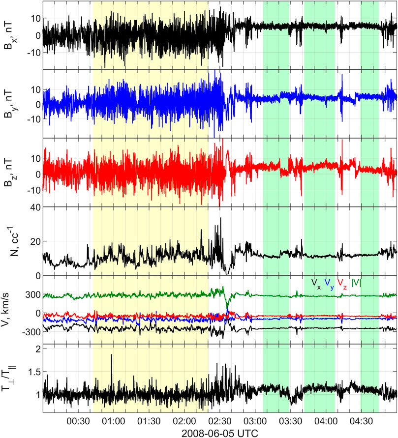
FIGURE 1. Overview of the event on 5 June 2008, 00:00–05:00 UTC observed by Cluster 3. From top to bottom: three components of the magnetic field; ion density; ion velocity components and magnitude; temperature anisotropy. The vectors are in GSE coordinate frame. The shaded areas indicate the sub-samples in the quasi-parallel (yellow) and quasi-perpendicular (green) regions.

First of all, the autocorrelation function $A_c(\mathrm{\Delta }t)=⟨B_i(t)B(t+\mathrm{\Delta }t)⟩/{\sigma }_{B_i}^2$ [33] was estimated in each sub-interval, for each field component B_i (with i = x, y, z) and for each of the four Cluster spacecraft after removing the mean, so that ${\sigma }_{B_i}^2$ indicates the variance of the field fluctuations. Since the results were found to be relatively independent of the chosen component and on the specific spacecraft, an average was estimated in order to improve the statistical convergence. The Figure 2A shows the averaged autocorrelation function for both samples, indicating a smooth decrease for the quasi-parallel sample, and a slower decay for the quasi-perpendicular case. In both cases, an e-folding estimate provided an autocorrelation timescale of $\sim 5$ s, a typical value for the magnetosheath plasma. The secondary peak near Δt ≃ 10 s, clearly observed in the quasi-perpendicular case, is likely due to the presence of waves typical of such configuration.

FIGURE 2

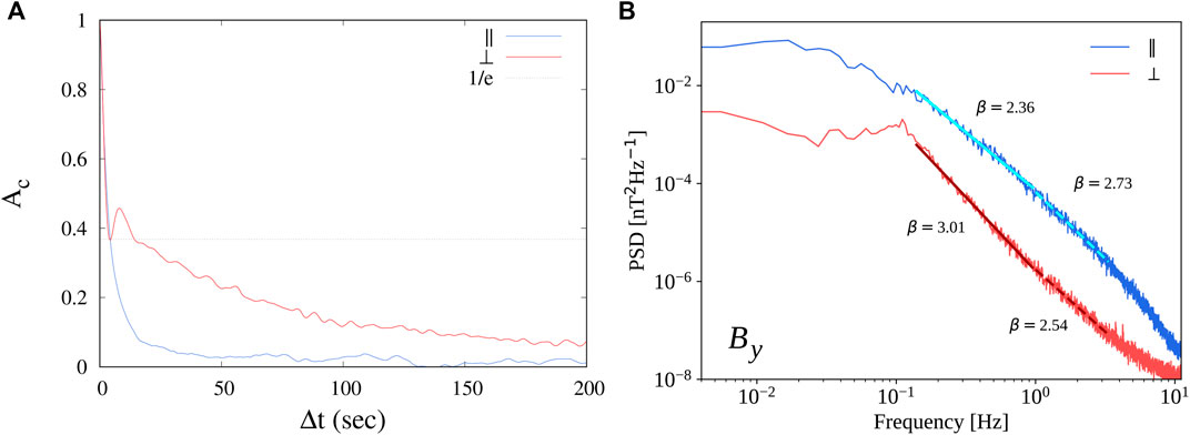
FIGURE 2. (A): autocorrelation function for the two samples, averaged over all components and all satellites. The correlation time, estimated as the 1/e value of the autocorrelation function, is roughly 5 s for both samples. (B): power spectral density/bf of the magnetic field B_y component measured by Cluster 2, for the quasi-parallel (‖, blue) and quasi-perpendicular ( ⊥, red) samples. Power-law fits are superposed in two frequency ranges: larger-scale range in full lines, and the smaller-scale range in dashed lines. A spectral break is identified at f ≃ 1 Hz. The respective spectral exponents are indicated, the fitting error being <0.03.

A similar study was performed for the magnetic power spectral density. The resulting averaged spectra are shown in the Figure 2B. The difference in the fluctuations energy is evident, with the quasi-parallel interval larger by at least one order of magnitude. For both cases, power-law scaling was found in two separate (larger- and smaller-scale) ranges. The spectral exponents obtained through a power-law fit are indicated in the figure, and are compatible with the typical kinetic turbulence scaling, usually observed at sub-ion scales in the solar wind, but commonly found in the magnetosheath. Looking at frequencies below 0.1 Hz shows that in the quasi-parallel samples a shallower Kolmogorov-like spectrum, with power-law scaling compatible with the typical 5/3, is present, and then a flattening indicates complete loss of correlations below 0.01 Hz. On the other hand, for the quasi-perpendicular intervals the Kolmogorov scaling has not formed yet, and decorrelation appears immediately below the peak at 0.1 Hz, likely due to the presence of waves. Such difference at low frequency is normally observed, with the quasi-parallel configuration plasma being typically more turbulent than for quasi-perpendicular configuration (see, e.g. [9]).

In order to characterize the presence of intermittency in the turbulence, the scale-dependent statistical properties of the two samples were studied by means for the two-times field increments ΔB_i(t, Δt) = |B_i(t + Δt) − B_i(t)|. The probability distribution functions (PDFs) of the standardized increments were then computed for timescales Δt ranging from the resolution scale dt up to a scale comparable with half the sub-samples size. As for the autocorrelation and spectral analysis, the statistical properties were observed to be roughly independent of both the component and the spacecraft, so that the PDFs shown in the Figures 3A,B are averaged over all sub-intervals, component and spacecraft. A reference standard Gaussian curve is also indicated. For the quasi-parallel sample, the typical change of PDF shape is observed. While the PDF is roughly Gaussian at large scale ($>46$ s), the tails become higher as the scale decreases (all the way down to the resolution scale dt), indicating an increasing presence of small-scale intense structures. This is the standard signature of intermittency. Note that in this case the tails of the PDF increase even in the absence of a Kolmogorov scaling, suggesting that some cascade mechanism is probably active even in the presence of kinetic or underdeveloped turbulence. The quasi-perpendicular sample shows variable PDF over a reduced range of scales, and the shape is much closer to Gaussian at all scales. This suggests that the turbulent cascade is less developed, and intermittency is still a minor effect. Finally, we have computed the field kurtosis $K(\mathrm{\Delta }t)=⟨\mathrm{\Delta }{B}_i^4⟩/{⟨\mathrm{\Delta }{B}_i^2⟩}^2$, a standard quantitative indicator of the deviation from Gaussian statistics [1]. Intermittency is often associated to the value of the kurtosis K_max at the bottom of the corresponding scaling range. However, a more correct interpretation is to estimate the scaling properties of kurtosis, which is directly related to the anomalous scaling of the field statistics. This can be done through a power-law fit of the kurtosis K(Δt) ∝Δt^−γ in each range where scaling is expected. The kurtosis scaling exponents γ can then be used as an indicator of the intermittency of the system, and for Navier-Stokes fluids may also be linked to the multifractal properties of turbulence [17,21,22]. Indeed, a faster increase of the kurtosis as the scale decreases corresponds to a more efficient emergence of localized, intermittent structures in the flow. The Figure 3C shows the scale dependence of the kurtosis for the two samples under study, averaged over the three magnetic field components and four Cluster satellites (again, only minor differences were observed for the different cases). A power-law fit was performed in the range 1–10 s, roughly corresponding to the larger-scale power-law range observed in the spectrum. The general behaviour is an increase toward smaller scales, although a transition region around the typical proton gyro-scale can be identified [34]. It is evident that the quasi-parallel sample has both larger maximum values ($K_{\max }^{\parallel }\simeq 8$ and $K_{\max }^{\perp }\simeq 4$) and faster increase (γ^∥ = 0.24 ± 0.04 and γ^⊥ = 0.10 ± 0.01) of the kurtosis, so that intermittency is larger than in the quasi-perpendicular sample. This confirms quantitatively the indication of the PDFs results that the quasi-parallel sample has more developed kinetic turbulence, while the quasi-parallel sample is only weakly intermittent. This difference may be due both to a less developed turbulence, or to the presence of disturbances such as waves and structures originated at the bow shock. Note that in the smaller-scale range, a different power-law is observed (not fitted), with a break corresponding to the spectral break seen in Figure 2. Such power-law scaling indicates that even in this range nonlinear interactions are actively generating small-scale turbulent structures. However, the energy transfer mechanisms appears to be slightly different than in the larger-scale range, as visible trough the slight change in scaling.

FIGURE 3

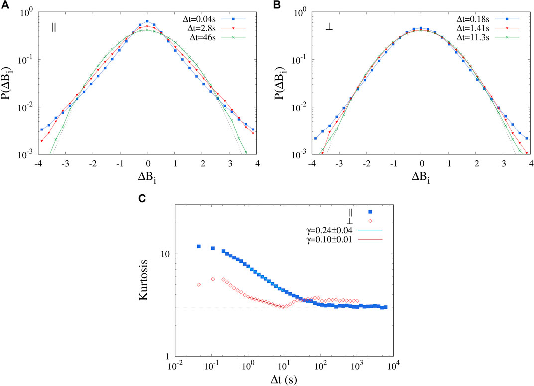
FIGURE 3. (A,B): scale-dependent PDFs of the magnetic field fluctuations, averaged over the four spacecraft and three components, and shown here at three different time lags. Gaussian reference curves are indicated as dashed lines. (A): quasi-parallel interval (‖); (B): quasi perpendicular interval (⊥). (C): kurtosis K of the scale-dependent magnetic field fluctuations, averaged over the three components and four satellites, for both intervals [quasi-parallel, ‖ and quasi-perpendicular, (⊥)]. A power-law fit K ∝Δt^−γ in the larger-scale range is indicated for both samples, and the scaling exponents γ are listed.

3 Multifractal Analysis of Magnetosheath Fluctuations

In the phenomenology of turbulence, fluctuations on all scales superpose in a highly disordered way. However, the small-scale fluctuations show the presence of sharp gradients whose characteristics are described by singularity scaling exponents [35]. As anticipated, while fractal, self-similar objects are well described by one singularity exponent, in turbulent fields intermittency introduces inhomogeneity of the fluctuations, so that the singularity exponent at a given point in space depends on the cross-scale transfer history at that location. Hence, a broad distribution of singularities is needed to fully describe the system’s properties. The distribution of singularity exponents, called the multifractal spectrum, represents one possible way to measure the exponent’s variability [36]. Wider multifractal spectra, which include more possible values of the singularity exponents necessary to describe the signal, correspond to stronger multifractality. The width of the multifractal spectrum can therefore quantitatively measure the variety of energy transfer channels, with more variability typically corresponding to enhanced intermittency [1]. A standard technique based on the multi-order scaling properties of the coarse-grained probability measure of the relevant field [29,35,37,38] is used here to obtain the multifractal spectrum of the two samples described above. This is typically based on the following steps.

1. Define an appropriate physical quantity for the analysis. This is typically a small-scale fluctuation, so that here we use the N-points time series of magnetic increments |ΔB_i(t, Δt)|, i = {1, … , N} [29] estimated at a time lag Δt ≃ 0.18 s, where spectra and kurtosis were observed to flatten for both samples (see previous Section). In multifractal analysis, both the squared and absolute value magnetic field increments are alternatively used. Here, we choose to use the absolute value to obtain better statistical convergence of the partition function.

2. Create a partition of the sample. This is done by generating M = T/Δt disjoint subsets of variable timescale Δt² labeled with j = {1, … , M}, where T is the sample duration.

3. Define a coarse-grained probability measure. For each of the subset of scale Δt, the associated probability measure is (see, e.g., [35], and references therein)

${\mu }_j\left(\mathrm{\Delta }t\right)=\frac{\sum _{i=\left(j-1\right)\mathrm{\Delta }t+1}^{j\mathrm{\Delta }t}|\mathrm{\Delta }B\left(i\right)|}{\sum _{i=1,N}|\mathrm{\Delta }B\left(i\right)|},(1)$

where the absolute value of all data values in each j-th box of size Δt is summed up, and normalized to the sum over the whole data set.

4. Use the measure defined above to estimate partition functions. For each scale Δt, these are defined as the sums over the M sub-samples of the q-th order powers of the measure[35],

${\chi }_q\left(\mathrm{\Delta }t\right)=\sum _{j=1}^M\mathrm{\Delta }t{\left[{\mu }_j\left(\mathrm{\Delta }t\right)\right]}^q,(2)$

where the number of sub-samples obviously depend on the scale. The partition functions amplify the scaling properties of the measure differently for different power exponent q, revealing the complexity of the general scaling of the field.

5. Identify singularities by determining the power-law scaling of the partition function. This can be done simply fitting the partition functions to a power-law of the scale, ${\chi }_q(\mathrm{\Delta }t)\propto \mathrm{\Delta }{t}^{{\tau }_q}$, and extracting the scaling exponents τ_q, which represent a quantitative measure of the multifractal properties of the field. For a fractal field, the exponent τ_q will behave like a linear function of the order q (e.g., in case of homogeneous dissipation and non-intermittent turbulence, where only one singularity exponent is sufficient to describes the whole system). Deviation from linearity is the result of the variability of the singularity exponents, or multifractality.

6. Finally, the multifractal spectrum can be obtained to provide an alternative description. The multifractal spectrum describes the local singularity exponent α and the corresponding fractal dimension f(α) of the subsets where the field has such singularity [35,37]. It can be obtained from the scaling exponents τ_q of the partition function using the Legendre transform α_q = dτ_q/dq and f(α) = qα_q − τ_q [19]. The width of f(α) gives a quantitative estimate of the strength of the multifractality [29].

For the two samples described in Section 2, the probability measures μ(Δt) and the partition functions χ_q (Δt) were estimated, using $q\in \left[-4:4\right]$, with step dq = 0.01. Examples of the partition functions are shown in the Figures 4A,B. Two power-law scaling ranges were identified above the proton gyro-scale and below or around the correlation scale, corresponding to the ranges identified in the spectra. Least-square power-law fits provided the values of the set of exponents τ_q for each of the two samples, shown in the Figures 4C,D for the two different ranges of scales. From these, the singularity spectra f(α) were also obtained (Figures 4E,F). The deviation from the fractal behavior, i.e. from linear dependence of τ_q, and from a single-valued f(α), is evident. While the analysis show that both samples are multifractal, considerable differences are present between the quasi-parallel and quasi-perpendicular intervals. In particular, in the larger range of scales a higher degree of multifractality, as evidenced for example by the broader distribution of singularity exponents, is clearly observed for the quasi-parallel sample, in agreement with the other estimators of intermittency discussed above. The quasi-perpendicular interval shows a nearly symmetric multifractal spectrum f(α), typical of random multiplicative processes. On the contrary, in the quasi-parallel interval the spectrum is more asymmetric, recalling non-multiplicative cascade processes, and more similar to spectra observed in the fully turbulent solar wind [29]. This is consistent with the steeper power spectrum and reduced intermittency observed in the quasi-perpendicular interval. All these observations suggest that the turbulence is more developed in the quasi-parallel interval, where it is closer to the standard solar-wind turbulence, while in the quasi-perpendicular case the cascade did not have enough time to fully develop after the shock crossing. In the smaller range of scales, the two intervals show more similar multifractal properties, in both cases presenting a broader singularity spectrum than at larger scales.

FIGURE 4

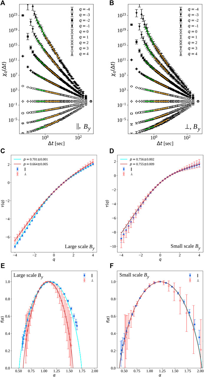
FIGURE 4. Example of multifractal analysis for the B_y component measured by Cluster 2. (A,B): partition function χ_q (Δt) in the quasi-parallel (A) and quasi-perpendicular (B) samples, for q indicated in the legend. Error bars are the standard deviation of the measure over the partition boxes (the argument of left-hand side of Eq. 2). Power-law fits are indicated in the larger-scale (yellow lines) and smaller-scale (green lines) ranges, with a break around Δt ≃ 1 s, noticeable for higher orders q. (C,D): scaling exponents τ_q versus the order q, in the larger (C) and smaller (D) ranges of scales, for quasi-parallel (‖) and quasi-perpendicular (⊥) intervals. Error bars are obtained through the power-law fit, and are slightly larger for the quasi-perpendicular interval. (E,F): the corresponding multifractal spectra f(α). Error bars are considerably amplified by the Legendre transformation. In (C–F), full lines represent the p-model (3) obtained fitting the scaling exponents τ_q.

In fully developed turbulence, the multifractal spectrum can be related through a Legendre transform to the anomalous scaling exponents of the structure functions (and therefore to the scaling of the kurtosis) [17]. Therefore, theoretical models of intermittency can extend to the multifractal spectrum and provide quantitative parameters. Here, we performed a fit of the scaling exponents τ_q with a p-model, a popular description of intermittency in the framework of a multiplicative, multifractal nonlinear turbulent cascade [39]. Originally developed for fluid turbulence, the p-model describes the cascade as the uneven redistribution of the energy associated to vortices of a given size and at one given position to a pair of daughter vortices. At each step of the cascade, the fraction of energy transferred to each of the two daughter structure is determined as a random number extracted from a binomial distribution, p and 1 − p, where 0 ≤ p ≤ 0.5. At small scale, the fraction of energy at a given position will be the result of a cascade of randomly distributed multipliers, resulting in intermittency. The fraction p is the parameter that describes the characteristics of the cascade. According to the original model [39], the scaling exponents τ_q can be modeled in terms of the parameter p as:

${\tau }_q=-{\mathit{log}}_2\left[p^q+{\left(1-p\right)}^q\right].(3)$

The multifractal nature of a turbulent field can thus be appropriately described by the model parameter p. For p ≃ 0.5, which indicates homogeneous redistribution of energy across scales, the system will be self-similar and thus mono-fractal. Smaller values are instead associated with increasingly inhomogeneous singularities, or multifractality. For the data-sets used here, the parameter p was obtained fitting the experimental exponents τ_q to the p-model, Eq. 3, in the two different ranges previously identified. Fits are shown as red and blue lines in Figure 4. In the large-scale range, the values obtained from the fit, also shown in Figure 5 (see description below), are p = 0.66 ± 0.02 (quasi-perpendicular) and p = 0.69 ± 0.01 (quasi-parallel). These values were obtained by averaging over the field components and four Cluster spacecraft (the uncertainty being the standard deviations), and are compatible with standard results for intermittency in fully developed inertial sub-range turbulence [39]. The quasi-parallel interval confirms a more pronounced multifractality, as expected according to the visual inspection of the multifractal spectra. On the other hand, at smaller scales both intervals give an average p = 0.76 ± 0.01, again compatible with strong intermittency of fluid turbulence, and with no difference between the two samples.

FIGURE 5

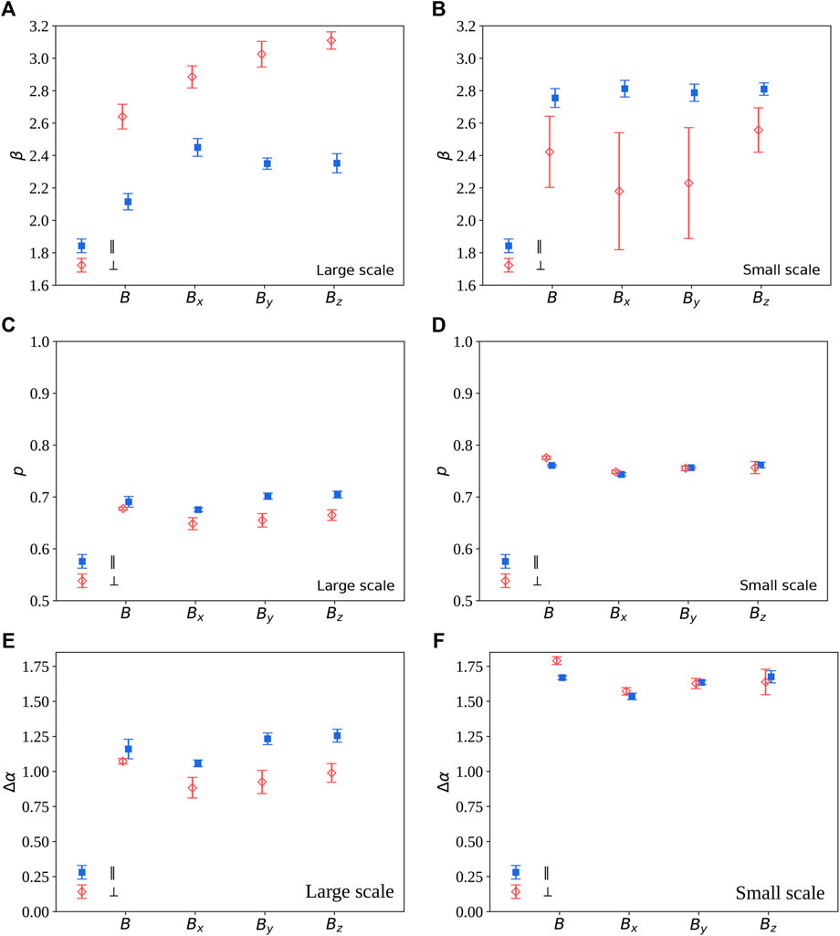
FIGURE 5. Visualization of the spectral exponent β (A,B), of the P-model parameter p (C,D), and of the multifractal width Δα (E,F), obtained for the magnetic field components in both intervals. Different colors and symbols refer to quasi-parallel (blue squares) and quasi-perpendicular (red diamonds) sub-intervals. Values are averaged over the four spacecraft, the error bar being the standard deviation. (E) refer to the large-scale range, (F) to the small-scale range.

Finally, a standard measure of multifractality was obtained by computing the width of the multifractal spectrum Δα = α_max − α_min [29]. This parameter indeed provides a fast estimate of the singularity variability of the time series. The observed values, shown in Figure 5 (see description below), are of the order of Δα ≃ 1.1 (quasi-parallel) or Δα ≃ 0.85 (quasi-perpendicular) for larger scales, and Δα ≃ 1.6 for smaller scales. Those values, obtained again as average over the different components and satellites, indicate strong multifractality (for comparison see, for example [29]), and confirm once again the difference between the two configurations only at larger scales, and the more enhanced multifractal nature of magnetic fluctuations at small scales.

Figure 5 shows a comparison of spectral exponent β (A,B), model parameter p (C,D) and multifractal width Δα (E,F) for the different magnetic field components and for its magnitude (conveniently distributed along the x-axis for visualization purposes), after averaging over the four Cluster spacecraft. In the larger scale range, all parameters show a neat difference between the two samples, consistent for all components (left panels). This quantitatively confirm the qualitative result that the quasi-parallel sample is more multifractal, and thus more intermittent, than the quasi-perpendicular sample. In the smaller-scale region, the spectral difference is still evident, while multifractality becomes similar, and stronger than in the larger-scale range. This is in agreement with the steeper increase of the kurtosis observed in this range with respect to larger scales, well visible in Figure3. The nature of such range of scales remains to be studied more in detail.

4 Conclusion

We have performed a multifractal analysis of two adjacent intervals of magnetosheath magnetic field measured by Cluster in 2008, showing a sharp transition from quasi-parallel to quasi-perpendicular geometry. After observing the spectral and intermittency properties, the multifractal spectrum was estimated using the standard box-counting technique. Results consistently show that each of the two samples has two separate scaling ranges, both with exponents larger than the typical Kolmogorov’s 5/3, suggesting that kinetic-scale turbulence is observed. In the fluid-scale inertial range, nonlinear interactions did not have enough time or energy to generate a cascade in the quasi-perpendicular interval. On the contrary, the initial formation of a short Kolmogorov-like spectrum is observed in the quasi-parallel case. This is in agreement with typical observations in the magnetosheath. In both ranges, intermittency is present, and the magnetic field is robustly multifractal, suggesting that the kinetic-scale turbulence is dominated by nonlinear interactions. In the larger range of scales, substantial differences are present between the quasi-parallel and quasi-perpendicular sub-intervals, with the former showing stronger intermittency and, accordingly, more multifractal fluctuations. These observations confirm the well-known fact that quasi-parallel intervals’ turbulence is stronger than in quasi-perpendicular intervals, and additionally reveal that, despite the fact that spectra are not Kolmogorov’s, nonlinear interactions are generating scale-dependent structures that are typical of a turbulent cascade. This is not the case in the strongly multifractal smaller-scale range, which however needs deeper analysis, left for future works. The observations presented here highlight the turbulent nature of magnetosheath magnetic fluctuations, and provide quantitative estimates of their multifractal properties. The specific sample measured by Cluster allowed the comparison between quasi-parallel and quasi-perpendicular configurations, revealing that near ion-scales the turbulence is fundamentally different in the two regions. This could be relevant for the correct modeling of the interactions between the solar wind and the magnetosphere, and in particular for the description of magnetic fluctuations in the magnetosheath.

Data Availability Statement

Publicly available datasets were analyzed in this study. This data can be found here: Cluster Science Archive: https://csa.esac.esa.int/csa-web.

Author Contributions

Conceptualization, LS-V and DB; formal analysis, AG, LS-V, and EY; supervision, LS-V, KE, OK, DK; interpretation, LS-V, DB, KE, EY, AG; writing: LS-V, DB, AG, and EY; funding acquisition, DB, KE, OK, DK, and EY.

Funding

This work has received support by the Perren Visiting Professorship at QMUL 2016, by the Italian CNR Short Term Mobility program 2016, by SNSA grants 86/20 and 145/18, and by Shota Rustaveli National Science Foundation Project N. FR17279.

Conflict of Interest

The authors declare that the research was conducted in the absence of any commercial or financial relationships that could be construed as a potential conflict of interest.

The reviewer XBC declared a past co-authorship with the author DB to the handling editor.

Publisher’s Note

All claims expressed in this article are solely those of the authors and do not necessarily represent those of their affiliated organizations, or those of the publisher, the editors and the reviewers. Any product that may be evaluated in this article, or claim that may be made by its manufacturer, is not guaranteed or endorsed by the publisher.

Footnotes

¹The Geocentric Solar Ecliptic (GSE) coordinates system has its x-axis pointing from the Earth towards the Sun, the y-axis lying in the ecliptic plane and pointing towards dusk, and the Z-axis parallel to the ecliptic pole.

²Note that from this point on Δt indicates a variable coarse-graining scale, and not the increment scale that is now fixed to a given value.

References

1. Frisch U. Turbulence. The Legacy of A. N. Kolmogorov. Cambridge, UK: Cambridge University Press (1995).

Google Scholar

2. Alexandrova O, Chen CHK, Sorriso-Valvo L, Horbury TS, Bale SD. Solar Wind Turbulence and the Role of Ion Instabilities. Space Sci Rev (2013) 178:101–39. doi:10.1007/s11214-013-0004-8

CrossRef Full Text | Google Scholar

3. Kolmogorov AN. The Local Structure of Turbulence in an Incompressible Viscous Fluid Forvery Large Reynolds Numbers. C.R Acad Sci USSR (1941) 30:301.

Google Scholar

4. Bruno R, Carbone V. The Solar Wind as a Turbulence Laboratory. Liv Rev Solar Phys (2013) 2. doi:10.12942/lrsp-2013-2

CrossRef Full Text | Google Scholar

5. Tu C-Y, Marsch E. MHD Structures, Waves and Turbulence in the Solar Wind: Observations and Theories. Space Sci Rev (1995) 73:1–210. doi:10.1007/bf00748891

CrossRef Full Text | Google Scholar

6. Sorriso-Valvo L, Carbone V, Giuliani P, Veltri P, Bruno R, Antoni V, et al. Intermittency in Plasma Turbulence. Planet Space Sci (2001) 49:1193–200. doi:10.1016/s0032-0633(01)00060-5

CrossRef Full Text | Google Scholar

7. Alexandrova O, Carbone V, Veltri P, Sorriso‐Valvo L. Small‐Scale Energy Cascade of the Solar Wind Turbulence. Astrophys J (2008) 674:1153–7. doi:10.1086/524056

CrossRef Full Text | Google Scholar

8. Echim M, Chang T, Kovacs P, Wawrzaszek A, Yordanova E, Narita Y, et al. Turbulence and Complexity of Magnetospheric Plasmas. In: R Maggiolo, editor. Magnetospheres in the Solar System. New York: Wiley (2021). p. 67–91. doi:10.1002/9781119815624.ch5

CrossRef Full Text | Google Scholar

9. Rakhmanova L, Riazantseva M, Zastenker G, Yermolaev Y, Lodkina I. Dynamics of Plasma Turbulence at Earth’s Bow Shock and through the Magnetosheath. Astrophys J (2020) 901(30):025004. doi:10.3847/1538-4357/abae00

CrossRef Full Text | Google Scholar

10. Yordanova E, Vörös Z, Raptis S, Karlsson T. Current Sheet Statistics in the Magnetosheath. Front Astron Space Sci (2020) 7:2. doi:10.3389/fspas.2020.00002

CrossRef Full Text | Google Scholar

11. Vörös Z, Yordanova E, Echim MM, Consolini G, Narita Y. Turbulence and Structures in the Terrestrial Magnetosheath. Astrophys J Lett (2016) 819:L15.

Google Scholar

12. Yordanova E, Vaivads A, André M, Buchert SC, Vörös Z. Magnetosheath Plasma Turbulence and its Spatiotemporal Evolution as Observed by the Cluster Spacecraft. Phys Rev Lett (2008) 100:205003. doi:10.1103/physrevlett.100.205003

PubMed Abstract | CrossRef Full Text | Google Scholar

13. Breuillard H, Yordanova E, Vaivads A, Alexandrova O. The Effects of Kinetic Instabilities on Small-Scale Turbulence in Earth's Magnetosheath. Astrophys J (2016) 829:54. doi:10.3847/0004-637x/829/1/54

CrossRef Full Text | Google Scholar

14. Karlsson T, Raptis S, Trollvik H, Nilsson H. Classifying the Magnetosheath behind the Quasiparallel and Quasi-Perpendicular bow Shock by Local Measurements. J Geophys Res (2021) 126:e2021JA029269. doi:10.1029/2021ja029269

CrossRef Full Text | Google Scholar

15. Dimmock AP, Osmane A, Pulkkinen TI, Nykyri K. A Statistical Study of the Dawn‐dusk Asymmetry of Ion Temperature Anisotropy and Mirror Mode Occurrence in the Terrestrial Dayside Magnetosheath Using THEMIS Data. J Geophys Res Space Phys (2015) 120:5489–503. doi:10.1002/2015ja021192

CrossRef Full Text | Google Scholar

16. Mandelbrot B. The Fractal Geometry of Nature. San Francisco: Freeman (1982).

Google Scholar

17. Frisch U, Parisi G. On the Singularity Structure of Fully Developed Turbulence. In: Turbulence and Predictability of Geophysical Flows and Climate Dynamics, Varenna Summer School LXXXVII (1983). p. 84.

Google Scholar

18. Benzi R, Paladin G, Parisi G, Vulpiani A. On the Multifractal Nature of Fully Developed Turbulence and Chaotic Systems. J Phys A: Math Gen (1984) 17:3521–31. doi:10.1088/0305-4470/17/18/021

CrossRef Full Text | Google Scholar

19. Halsey TC, Jensen MH, Kadanoff LP, Procaccia I, Shraiman BI. Fractal Measures and Their Singularities: The Characterization of Strange Sets. Phys Rev A (1986) 33:1141–51. doi:10.1103/physreva.33.1141

CrossRef Full Text | Google Scholar

20. Ott E. Chaos in Dynamical Systems. Cambridge, U. K.: Cambridge Univ. Press (1993).

Google Scholar

21. Castaing B, Gagne Y, Hopfinger EJ. Velocity Probability Density Functions of High Reynolds Number Turbulence. Physica D: Nonlinear Phenomena (1990) 46:177–200. doi:10.1016/0167-2789(90)90035-n

CrossRef Full Text | Google Scholar

22. Sorriso-Valvo L, Marino R, Lijoi L, Perri S, Carbone V. Self-consistent Castaing Distribution of Solar Wind Turbulent Fluctuations. Astrophys J (2015) 807:86. doi:10.1088/0004-637x/807/1/86

CrossRef Full Text | Google Scholar

23. Burlaga LF. Multifractal Structure of the Interplanetary Magnetic Field: Voyager 2 Observations Near 25 AU, 1987-1988. Geophys Res Lett (1991) 18:69–72. doi:10.1029/90gl02596

CrossRef Full Text | Google Scholar

24. Macek WM. Modeling Multifractality of the Solar Wind. Space Sci Rev (2006) 122:329–37. doi:10.1007/s11214-006-8185-z

CrossRef Full Text | Google Scholar

25. Marsch E, Tu C-Y, Rosenbauer H. Multifractal Scaling of the Kinetic Energy Flux in Solar Wind Turbulence. Ann Geophys (1996) 14:259–69. doi:10.1007/s00585-996-0259-4

CrossRef Full Text | Google Scholar

26. Macek WM, Szczepaniak A. Generalized Two-Scale Weighted Cantor Set Model for Solar Wind Turbulence. Geophys Res Lett (2008) 35:L02108. doi:10.1029/2007gl032263

CrossRef Full Text | Google Scholar

27. Sorriso-Valvo L, Carbone F, Leonardis E, Chen CHK, Šafránková J, Němeček Z. Multifractal Analysis of High Resolution Solar Wind Proton Density Measurements. Adv Space Res (2017) 59:1642–51. doi:10.1016/j.asr.2016.12.024

CrossRef Full Text | Google Scholar

28. Burlaga LF. Multifractal Structure of the Large-Scale Heliospheric Magnetic Field Strength Fluctuations Near 85AU. Nonlin Process. Geophys (2004) 11:441–5. doi:10.5194/npg-11-441-2004

CrossRef Full Text | Google Scholar

29. Macek WM, Wawrzaszek A, Carbone V. Observation of the Multifractal Spectrum in the Heliosphere and the Heliosheath by Voyager 1 and 2. J Geophys Res (2012) 117:A12101. doi:10.1029/2012ja018129

CrossRef Full Text | Google Scholar

30. Wawrzaszek A, Echim M, Macek WM, Bruno R. Evolution of Intermittency in the Slow and Fast Solar Wind beyond the Ecliptic Plane. Astrophys J Lett (2015) 814:L19.

CrossRef Full Text | Google Scholar

31. Macek WM, Wawrzaszek A, Burlaga LF. Multifractal Structures Detected by Voyager 1 at the Heliospheric Boundaries. Astrophys J (2014) 793:L30. doi:10.1088/2041-8205/793/2/l30

CrossRef Full Text | Google Scholar

32. Yordanova E, Grzesiak M, Wernik AW, Popielawska B, Stasiewicz K. Multifractal Structure of Turbulence in the Magnetospheric Cusp. Ann Geophys (2004) 22:2431–40. doi:10.5194/angeo-22-2431-2004

CrossRef Full Text | Google Scholar

33. Papoulis A, Pillai SU. Probability, Random Variables and Stochastic Processes. New York, USA: McGraw-Hill (1991).

Google Scholar

34. Chen CHK, Sorriso-Valvo L, Šafránková J, Němeček Z. Intermittency of Solar Wind Density Fluctuations from Ion to Electron Scales. Astrophys J (2014) 789:L8. doi:10.1088/2041-8205/789/1/l8

CrossRef Full Text | Google Scholar

35. Paladin G, Vulpiani A. Anomalous Scaling Laws in Multifractal Objects. Phys Rep (1987) 156:147–225. doi:10.1016/0370-1573(87)90110-4

CrossRef Full Text | Google Scholar

36. Sreenivasan KR. Fractals and Multifractals in Fluid Turbulence. Annu Rev Fluid Mech (1991) 23:539–604. doi:10.1146/annurev.fl.23.010191.002543

CrossRef Full Text | Google Scholar

37. Chhabra AB, Meneveau C, Jensen RV, Sreenivasan KR. Direct Determination of the F(α) Singularity Spectrum and its Application to Fully Developed Turbulence. Phys Rev A (1989) 40:5284–94. doi:10.1103/physreva.40.5284

CrossRef Full Text | Google Scholar

38. Leonardis E, Sorriso-Valvo L, Valentini F, Servidio S, Carbone F, Veltri P. Multifractal Scaling and Intermittency in Hybrid Vlasov-Maxwell Simulations of Plasma Turbulence. Phys Plasmas (2016) 23:022307. doi:10.1063/1.4942417

CrossRef Full Text | Google Scholar

39. Meneveau C, Sreenivasan KR. Simple Multifractal cascade Model for Fully Developed Turbulence. Phys Rev Lett (1987) 59:1424–7. doi:10.1103/physrevlett.59.1424

PubMed Abstract | CrossRef Full Text | Google Scholar