Optimal Resonances in Multiplex Neural Networks Driven by an STDP Learning Rule

1 Introduction

Spiking activity in neural systems can be induced and affected by noise, which can be internally produced by the system itself and/or externally by processes acting on the system. The sources of neural noise include 1) synaptic noise, which is externally produced, and is caused by the quasi-random release of neurotransmitters by synapses and/or random synaptic input from other neurons, and 2) channel noise, which is internally produced and comes from the random switching of ion channels [47, 49]. Synaptic and channel noise have been found to give rise to peculiar dynamical behavior in neural networks, including various resonance phenomena. The most prominent forms of these noise-induced resonance phenomena include: stochastic resonance (SR) [3, 28], coherence resonance (CR) [36], self-induced stochastic resonance (SISR) [10, 34], and inverse stochastic resonance (ISR) [18, 42]. The emergence and the dynamics of SR, CR, SISR, and ISR are quite different from each other, and therefore, they have mostly been separately investigated in previous research works. It might nevertheless be possible that fundamental relationships exist between some or even all of these noise-induced resonances and that efficient enhancement schemes for information processing could emerge from their co-existence in a neural network. Some research works have shown intriguing results about the interplay between some of these noise-induced resonance phenomena. The bifurcation and stochastic analysis in [48] revealed that the parameter that changes the relative geometric positioning (and stability) of the fixed point (the quiescent state of the neuron) with respect to the fold point of the cubic nullcline of the FitzHugh-Nagumo (FHN) model [11] can cause a switch between SISR and ISR in the same synaptic weak-noise limit. Experiments have frequently shown that real biological neurons with similar physiological features, excited by identical stimuli, may spike quite differently, thus expressing different neuro-computational properties [40]. The analysis presented in [48] may, therefore, provide a qualitative explanation for this particular behavior. Zamani et al. [51] later showed a similar behavior between SR and ISR in a minimal bistable spiking neural circuit, where both mechanisms could co-exist under careful preparations of the neural circuit. Whether and if so, how all of these different types of noise-induced resonance mechanisms are related and what efficient enhancement schemes for information processing emerge from their interactions is far from being completely understood.

In this paper, CR and SISR will be the phenomena of interest. In fact, in both CR and SISR, small random perturbations of an excitable neural system with a large time scale separation ratio may lead to the emergence of coherent spiking activity. The mechanisms behind these noise-induced resonance phenomena, however, are entirely different, see [10]. CR [36] occurs when a maximal degree of regularity in the neuron’s spiking activity is achieved at an optimal noise intensity without a periodic input signal, provided the neuron’s bifurcation parameters are tuned near the Hopf bifurcation [25, 26, 36] or the saddle-node bifurcation [17, 19, 20, 27] threshold. In this case, a relatively small noise amplitude can easily (without overwhelming the entire dynamics) drive the neuron towards a coherent spiking activity that emerges right after the bifurcation threshold. Thus, during CR, noise plays a relatively passive role. In the FitzHugh-Nagumo neuron model (that will be used in this work), CR requires that the noise source is attached to the slow recovery variable—mimicking the dynamics of channel noise [10].

SISR, on the other hand, occurs when a vanishingly small noise intensity perturbing the fast variable of an excitable system results in the onset of a limit cycle behavior that is absent without noise [34]. SISR combines a coherence resonance-type mechanism with an intrinsic reset mechanism, and no external periodic driving is required. The period of the coherent oscillations created by the noise has a non-trivial dependence on the noise intensity and the timescale between the fast variable and slow variable of the excitable system. SISR essentially depends on the interplay between three different timescales: the two timescales of the deterministic part of the excitable system (i.e., the fast and slow timescale of the fast and slow variable, respectively), plus a third timescale characteristic of the noise, which plays an active role in the mechanism of SISR, in contrast to CR. Thus, the mechanism behind SISR is different from that of CR (see [10]), and remarkably, it can also occur away from bifurcation thresholds in a parameter regime where the zero-noise (deterministic) dynamics do not display a limit cycle nor even its precursor. The properties of the limit cycle that SISR induces are controlled by both the noise intensity and the time scale separation ratio. Moreover, unlike CR, SISR requires a strong timescale separation ratio between the variables of the excitable system. In the FitzHugh-Nagumo neuron model, SISR (in contrast to CR) requires that the noise source is attached to the fast membrane potential variable—mimicking the dynamics of synaptic noise [10].

Of course, it is worth pointing out that a neuron can have both channel and synaptic noise simultaneously. In this case, CR and SISR will compete with each other. The dominant phenomenon will correspond to the one whose conditions are met first. It is shown in [10, 34] that SISR will dominate CR because the oscillations due to SISR are contained in those of CR. Thus, the conditions necessary for SISR can always be met first. In the current work, we shall not consider the situations where we have both channel and synaptic noise in a given layer. Just one type of noise will be considered in a given layer, and thus the competition between CR and SISR in a given layer will also not be considered.

The characteristic features of CR and SISR based on (1) time-delayed feedback couplings and network topology [1, 15, 30], 2) the multiplexing of layer networks [6, 31, 39, 46, 50], and 3) the use of one type of noise-induced resonance mechanism to optimize another type [50] have been established. It has been shown that appropriate selection of the time-delayed feedback parameters of FHN neurons coupled in a ring network can modulate CR: with a local coupling topology, synaptic time delay weakens CR, while in cases of non-local and global coupling, only appropriate synaptic time delays can strengthen or weaken CR [1, 15, 30, 38]. The enhancement of CR and SISR in neural systems with multiplex layer networks has recently attracted attention. In a multiplex network [5], the nodes participate in several networks simultaneously, and the connections and interaction patterns are different in the different networks, although the nodes preserve their identities across the different networks or layers. Since there may exist different types of relations between neurons or brain regions, multiplex networks have also been proposed as neurophysiological models [8]. For instance, functional couplings, like synchronization, between brain regions can be realized in different frequency bands. And each such frequency band can process a different type of information, for instance in language processing, phonetic, semantic and prosodic information [13]. But the main purpose of our paper is a formal investigation of the interplay between different types of stochastic resonance in a model where the individual units follow FHN dynamics, as FHN has become a paradigmatic model system for nonlinear dynamics [24] where many features can be studied in rather explicit terms.

In particular, the enhancement of CR in one layer of a multiplex network of FHN neurons based on the occurrence of SISR in another layer was established in [50]. In this case, two enhancement schemes for CR were compared: In one scheme (CR-CR scheme), one layer of the multiplex network is configured so that CR is optimal and the other layer configured so that CR is non-optimal in isolation. In the other scheme (SISR-CR scheme), one layer of the multiplex network is configured so that SISR is optimal, and the other layer is configured so that CR is non-optimal in isolation. It was then shown that depending on which optimal resonance mechanism (CR or SISR) we had in one layer of the multiplex network, the best enhancement of CR in the other layer would depend on the multiplexing time delay and strength between the two layers. With weaker multiplexing strength and shorter time delays between the layers, the CR-CR scheme performs better than the SISR-CR scheme. But with stronger multiplexing connections, the SISR-CR scheme outperforms the CR-CR scheme, especially at weaker noise amplitudes and longer multiplexing time delays. This result suggests that the interactions between different noise-induced resonance mechanisms in neural networks could open up new possibilities for control and enhancement of information processing. These enhancement schemes could allow us to enhance information processing in neural networks more efficiently, using the interplay between different noise-induced resonance mechanisms and the multiplexing of layer networks. Enhancement schemes based on multiplexing (or, in general, on connecting several layers to form a multilayer network) are advantageous because the dynamics of one layer can be controlled by adjusting the parameters of another layer. So far, the enhancement of CR and SISR based on the multiplexing of neural layer networks has been established only in regular networks in the absence of STDP [6, 31, 39, 46, 50].

Adaptive (or learning) rules in biological neural networks have been linked to an important mechanism, namely, spike-timing-dependent plasticity (STDP) [16, 29]. STDP describes how the synaptic weights get modified by repeated pairings of pre-and postsynaptic action potentials (spikes) with the sign and the degree of the modification dependent on the relative timing of the firing of neurons. Depending on the precise timing of pre-and postsynaptic action potentials, the synaptic weights can exhibit long-term potentiation (LTP, i.e., persistent strengthening of synapses) or long-term depression (LTD, i.e., persistent weakening of synapses). There are two main types of STDP—Hebbian excitatory STDP (eSTDP) and anti-Hebbian inhibitory STDP (iSTDP). In this paper, we will focus only on eSTDP.

The ubiquity and importance of STDP in neural dynamics require us to investigate the enhancement of CR and SISR in adaptive neural networks driven by STDP. Such an investigation should be instrumental both theoretically and experimentally. Some previous works have shown the crucial role of adaptivity in network of coupled oscillators. For example, in [2] it is shown that the plasticity of the connections between oscillators plays a facilitatory role for inverse stochastic resonance (ISR), where adaptive couplings guide the dynamics of coupled oscillators to parameter domains in which noise effectively enhances ISR. In [12], it is shown how the interaction of noise and multiscale dynamics, induced by slowly adapting feedback, may affect an excitable system, giving rise to a new mode of behavior based on switching dynamics which allows for an efficient control of the properties of CR.

In the current work, the main questions we want to address are the following: 1) How do network topology and STDP parameters affect the degree of coherence due to CR and SISR? 2) In the presence of STDP, which of these noise-induced resonance phenomena is more robust to parametric perturbations? 3) In the presence of STDP, is an enhancement of the less robust phenomenon in an isolated layer network still possible via multiplexing? 4) Can the occurrence of one resonance phenomenon in one layer be used to enhance the other phenomenon in another layer in the presence of STDP? 5) If the answers to the previous questions are affirmative, then what behavior (LTP or LTD) of the STDP learning rule optimizes the multiplexing enhancement strategy?

Here is an outline of the remainder of this article: In Section 2, we present the mathematical model of the stochastic neural networks and give a brief description of the STDP learning rule and the dynamical differences in the emergent nature of the two noise-induced resonance phenomena that are of interest. In Section 3, we present the numerical methods used in our numerical simulations. In Section 3.1, we discuss the results of the dynamics of CR and SISR in isolated layer networks. In Section 3.2, we discuss the results of the enhancement of SISR using the multiplexing technique. Finally, we summarize our findings and conclude in Section 4.

2 Mathematical Model

We consider the following two-layer multiplex network, where each layer represents a network of N diffusively coupled FHN neurons in the excitable regime and the presence of noise:

$\left\{\begin{array}{cc}d{v}_{1i}\hfill & =\left[v_{1i}-\frac{v_{1i}^3}{3}-w_{1i}-I_{1i}^s\left(t\right)+I_{2i}^m\left(t\right)\right]dt+{\sigma }_{1}d{W}_{1i},\hfill \\ d{w}_{1i}\hfill & =\left[{\epsilon }_1\left(v_{1i}+\alpha -{\gamma }_1{w}_{1i}\right)\right]dt+{\sigma }_{2}d{W}_{2i},\hfill \\ d{v}_{2i}\hfill & =\left[v_{2i}-\frac{v_{2i}^3}{3}-w_{2i}-I_{2i}^s\left(t\right)+I_{1i}^m\left(t\right)\right]dt+{\widehat{\sigma }}_{1}d{W}_{3i},\hfill \\ d{w}_{2i}\hfill & =\left[{\epsilon }_2\left(v_{2i}+\alpha -{\gamma }_2{w}_{2i}\right)\right]dt+{\widehat{\sigma }}_{2}d{W}_{4i},\hfill \end{array}\right.(1)$

$v_{1i}\in \mathbb{R}$ and $w_{1i}\in \mathbb{R}$ represent the fast membrane potential variables and the slow recovery current variables in the first layer, respectively. Similarly, $v_{2i}\in \mathbb{R}$ and $w_{2i}\in \mathbb{R}$, respectively represent the membrane potential and recovery current variables for the neurons in the second layer. The index i = 1, … , N stands for the ith neuron in the network of N neurons. 0 < ɛ₁ ≪ 1 and 0 < ɛ₂ ≪ 1 are the time-scale separation ratios between the fast membrane potential and the slow recovery current variables in the first and second layers, respectively. γ₁ > 0 and γ₂ > 0 are co-dimension-one Hopf bifurcation parameters in each of the layers and thus define the excitability threshold. α ∈ (0, 1) is a constant parameter. σ₁W_1i is the uncorrelated Gaussian white noise with standard deviation σ₁, and similarly for ${\sigma }_2{W}_{2i},{\widehat{\sigma }}_1{W}_{3i}$, and ${\widehat{\sigma }}_2{W}_{4i}$. σ₁W_1i and ${\widehat{\sigma }}_1{W}_{3i}$ which are attached to the fast membrane potential variables should be interpreted as representing synaptic noise sources, while σ₂W_2i and ${\widehat{\sigma }}_2{W}_{4i}$ which are attached to the slow recovery variables both represent channel noise sources.

The terms $I_{1i}^s(t)$, $I_{2i}^s(t)$, $I_{1i}^m(t)$, and $I_{2i}^m(t)$ in Eq. 1 represent synaptic currents (modelled by diffusive electrical couplings) and also govern the STDP learning rule between connected neurons. We point out that we are using adaptive (based on STDP) electrical synapses so that we can directly compare our results to those in [50] where non-adaptive electrical synapses are used to study CR and SISR. The intra-layer synaptic currents $I_{1i}^s(t)$ and $I_{2i}^s(t)$ of the ith neuron in the layer 1 and layer 2 at time t are respectively given by

$\left\{\begin{array}{c}{I}_{1i}^s\left(t\right)=\frac{1}{c_i^1}\sum _{j\ne i}{a}_{ij}^1{K}_{ij}^1\left(t\right)\left(v_{1j}\left(t-{\tau }_1\right)-v_{1i}\left(t\right)\right),\hfill \\ I_{2i}^s\left(t\right)=\frac{1}{c_i^2}\sum _{j\ne i}{a}_{ij}^2{K}_{ij}^2\left(t\right)\left(v_{2j}\left(t-{\tau }_2\right)-v_{2i}\left(t\right)\right),\hfill \end{array}\right.(2)$

where the synaptic connectivity matrices $A^1={\{a_{ij}^1\}}_{i,j=1}^N$ and $A^2={\{a_{ij}^2\}}_{i,j=1}^N$ of the layer 1 and layer 2, respectively, have $a_{ij}^1=1=a_{ij}^2$ if the neuron j is pre-synaptic to the neuron i; otherwise, $a_{ij}^1=0=a_{ij}^2$. The synaptic connections in each layer, represented by the connectivity matrices A¹ and A², are modeled in terms of the time-invariant Watts-Strogatz small-world network [41, 43, 44], where the in-degree of the ith neuron in the ℓth layer (i.e., the number of synaptic inputs to the neuron i in layer ℓ) is given by $c_i^{\ell }={\sum }_{j\ne i}{a}_{ij}^{\ell }$, (ℓ = 1, 2). The intra-layer time delays of the electric synaptic coupling in layer 1 and layer 2 are represented by τ₁ and τ₂, respectively.

The inter-layer synaptic currents $I_{1i}^m(t)$ and $I_{2i}^m(t)$ (which we shall also sometimes refer to as multiplexing currents) of the ith neuron in layer 1 and layer 2 at time t are respectively given by

$\left\{\begin{array}{c}{I}_{1i}^m\left(t\right)=K_{ii}^{12}\left(t\right)\left(v_{2i}\left(t-{\tau }_{12}\right)-v_{1i}\left(t\right)\right),\hfill \\ I_{2i}^m\left(t\right)=K_{ii}^{12}\left(t\right)\left(v_{1i}\left(t-{\tau }_{12}\right)-v_{2i}\left(t\right)\right),\hfill \end{array}\right.(3)$

where τ₁₂ represents the multiplexing (inter-layer) time delay of the electrical synaptic coupling between layer 1 and layer 2. With increasing time t, the intra-layer synaptic strengths $K_{ij}^1(t)$ and $K_{ij}^2(t)$, and the multiplexing (inter-layer) synaptic strength $K_{ii}^{12}(t)$ for each synapse are updated with a nearest-spike pair-based STDP rule [33]. To prevent unbounded growth, negative conductances (i.e., negative coupling strength) and elimination of synapses (i.e., $K_{ij}^1=K_{ij}^2=K_{ii}^{12}=0$), we set a range with the lower and upper bounds: $\{K_{ij}^1,K_{ij}^2,K_{ii}^{12}\}\in [0.0001,1]$. The initial intra-layer synaptic weights (i.e., $K_{ij}^1(t=0)$ and $K_{ij}^2(t=0)$), are normally distributed with mean and standard deviation equal to 0.1 and 0.02, respectively. And each of the N initial inter-layer synaptic weights $K_{ii}^{12}(t=0)$ is uniformly distributed in the interval [0.0001, 1]. They are updated according to the rule

$\left\{\begin{array}{c}{K}_{ij}^1\to K_{ij}^1+\lambda \mathrm{\Delta }{K}_{ij}^1\left(\mathrm{\Delta }{t}_{ij}^1\right),\hfill \\ K_{ij}^2\to K_{ij}^2+\lambda \mathrm{\Delta }{K}_{ij}^2\left(\mathrm{\Delta }{t}_{ij}^2\right),\hfill \\ K_{ii}^{12}\to K_{ii}^{12}+\lambda \mathrm{\Delta }{K}_{ii}^{12}\left(\mathrm{\Delta }{t}_{ii}^{12}\right),\hfill \end{array}\right.(4)$

The intra-layer synaptic modifications $\mathrm{\Delta }{K}_{ij}^1(\mathrm{\Delta }{t}_{ij}^1)$ and $\mathrm{\Delta }{K}_{ij}^2(\mathrm{\Delta }{t}_{ij}^2)$ depend on the relative time difference $\mathrm{\Delta }{t}_{ij}=(t_i^{(post)}-t_j^{(pre)})$ $(\mathrm{\Delta }{t}_{ij}=\mathrm{\Delta }{t}_{ij}^1,\mathrm{\Delta }{t}_{ij}^2)$ between the nearest-spike times of the post-synaptic neuron i and the pre-synaptic neuron j. The inter-layer synaptic modification $\mathrm{\Delta }{K}_{ii}^{12}(\mathrm{\Delta }{t}_{ii}^{12})$ depends on the relative time difference $\mathrm{\Delta }{t}_{ii}^{12}=(t_2^{(post)}-t_1^{(pre)})$ between the nearest-spike times of the ith post-synaptic neuron in layer 2 and the ith pre-synaptic neuron in layer 1. The parameter λ represents the learning rate. It was found that small learning rates lead to more robust learning [32]. Hence, in this work, we choose a small learning rate (i.e., λ = 0.0001) which, by the way, also simulates the effect of STDP on the long-term evolution of a neural network [37]. In the numerical simulations, we will consider eSTDP with an asymmetric Hebbian time window for the synaptic modifications given by [4, 22]:

$\left\{\begin{array}{c}\mathrm{\Delta }{K}_{ij}^1\left(\mathrm{\Delta }{t}_{ij}^1\right)=\left\{\begin{array}{c}{P}_1\exp \left(-\mathrm{\Delta }{t}_{ij}^1/{\tau }_{1p}\right)\text{if}\mathrm{\Delta }{t}_{ij}^1>0\hfill \\ -D_1\exp \left(\mathrm{\Delta }{t}_{ij}^1/{\tau }_{1d}\right)\text{if}\mathrm{\Delta }{t}_{ij}^1<0\hfill \\ 0,\text{if}\mathrm{\Delta }{t}_{ij}^1=0\hfill \end{array}\right.\hfill \\ \mathrm{\Delta }{K}_{ij}^2\left(\mathrm{\Delta }{t}_{ij}^2\right)=\left\{\begin{array}{c}{P}_2\exp \left(-\mathrm{\Delta }{t}_{ij}^2/{\tau }_{2p}\right)\text{if}\mathrm{\Delta }{t}_{ij}^2>0\hfill \\ -D_2\exp \left(\mathrm{\Delta }{t}_{ij}^2/{\tau }_{2d}\right)\text{if}\mathrm{\Delta }{t}_{ij}^2<0\hfill \\ 0,\text{if}\mathrm{\Delta }{t}_{ij}^2=0\hfill \end{array}\right.\hfill \\ \mathrm{\Delta }{K}_{ii}^{12}\left(\mathrm{\Delta }{t}_{ii}^{12}\right)=\left\{\begin{array}{c}{P}_{12}\exp \left(-\mathrm{\Delta }{t}_{ii}^{12}/{\tau }_{\mathit{12p}}\right)\text{if}\mathrm{\Delta }{t}_{ii}^{12}>0\hfill \\ -D_{12}\exp \left(\mathrm{\Delta }{t}_{ii}^{12}/{\tau }_{\mathit{12d}}\right)\text{if}\mathrm{\Delta }{t}_{ii}^{12}<0\hfill \\ 0\text{if}\mathrm{\Delta }{t}_{ii}^{12}=0,\hfill \end{array}\right.\hfill \end{array}\right.(5)$

where LTP occurs if $\mathrm{\Delta }{t}_{ij}^1>0$, $\mathrm{\Delta }{t}_{ij}^2>0$, and $\mathrm{\Delta }{t}_{ii}^{12}>0$ (i.e., a post-synaptic spike follows a pre-synaptic spike); LTD if $\mathrm{\Delta }{t}_{ij}^1<0$, $\mathrm{\Delta }{t}_{ij}^2<0$, and $\mathrm{\Delta }{t}_{ii}^{12}<0$ (i.e., a post-synaptic spike precedes a pre-synaptic spike); and no synaptic modification if $\mathrm{\Delta }{t}_{ij}^1=\mathrm{\Delta }{t}_{ij}^2=\mathrm{\Delta }{t}_{ii}^{12}=0$. In Eq. 5, P₁, P₂, and P₁₂ (D₁, D₂, and D₁₂) represent the potentiation (depression) adjusting rate parameters in layer 1, layer 2, and between layer 1 and 2, respectively. And τ_1p, τ_2p, and τ_12p (τ_1d, τ_2d, and τ_12d) represent the potentiation (depression) temporal window parameters in layer 1, layer 2, and between layer 1 and 2, respectively. The amount of synaptic modification (i.e., strengthening or weakening) is controlled by the adjusting rate parameters P₁, P₂, P₁₂, D₁, D₂, and D₁₂, while the time window for the synaptic modification is controlled by τ_1p, τ_2p, τ_12p, τ_1d, τ_2d, and τ_12d.

Experimental investigations [7, 9, 14, 45, 52] have shown that for a fixed stimulus, D₁τ_1d > P₁τ_1p ensures dominant depression of synapses, otherwise (i.e., D₁τ_1d ≤ P₁τ_1p) dominant potentiation. In Figures 1A,B, we show the asymmetric Hebbian time window for the synaptic modification $\mathrm{\Delta }{K}_{ij}^1(\mathrm{\Delta }{t}_{ij})$ given by Eq. 5 ($\mathrm{\Delta }{K}_{ij}^2(\mathrm{\Delta }{t}_{ij}^2)$ and $\mathrm{\Delta }{K}_{ii}^{12}\left(\mathrm{\Delta }{t}_{ii}^{12}\right.$ have the same behavior). We see that $\mathrm{\Delta }{K}_{ij}^1(\mathrm{\Delta }{t}_{ij})$ varies, depending on the relative time difference $\mathrm{\Delta }{t}_{ij}^1$ between the nearest spike times of the post-synaptic neuron i and the pre-synaptic neuron j. In Figure 1A, for a fixed value of D₁ (= 0.5), τ_1d (= 20), and τ_1p (= 20), we show the effects of P₁ on LTP and LTD. In Figure 1B, for a fixed value of D₁ (= 0.5), τ₁(= 20), and P₁ (= 0.5), we show the effects of τ_1d on LTP and LTD. In the same way, fixing P₁ and τ_1d and varying D₁ and τ_1p show similar effects on LTD and LTP. Thus, for a particular noise intensity, when we fix parameter values of D₁ and τ_1p, the inequality D₁τ_1d > P₁τ_1p (D₁τ_1d ≤ P₁τ_1p) can switch from LTD (LTP) to LTP (LTD) by changing the values of the parameters P₁ and τ_1d. Hence, the synapses can exhibit LTD and LTP if we vary only two parameters (i.e., P₁ and τ_1d or D₁ and τ_1p) and keep the other two constant. Therefore, throughout our studies, we fix the depression adjusting rate parameter at D₁ = 0.5 and the potentiation temporal window parameter at τ_1p = 20, and choose the potentiation adjusting rate parameter P₁ ∈ [0.1, 1] and the depression temporal window parameter τ_1d ∈ [0.2, 30] as the alterable (control) parameters of the eSTDP learning rule.

FIGURE 1

FIGURE 1. Time windows for an asymmetric Hebbian eSTDP learning rule. Plot of synaptic modification $\mathrm{\Delta }{K}_{ij}^1$ versus $\mathrm{\Delta }{t}_{ij}^1(=t_i^{(post)}-t_j^{(pre)})$. $t_i^{(post)}$ and $t_j^{(pre)}$ are spiking times of the ith post-synaptic and the jth pre-synaptic neurons, respectively. The blue and magenta curves represent LTP, while the red and cyan curves represents LTD. Th effects of P₁ and τ_1d on LTD and LTP are indicated in panels (A) and (B), respectively. The other eSTDP parameters are fixed at: D₁ = 0.5, τ_1p = 20.

3 Numerical Results

To quantify the degree of SISR (i.e., the degree of coherence of the spiking activity induced by the mechanism of SISR), we use the normalized standard deviation of the mean interspike interval, commonly known as the coefficient of variation [36]. Because the coefficient of variation is based on the time intervals between spikes, it does relate to the timing precision of information processing in neural systems [35] and naturally becomes an essential statistical measure in neural coding. The coefficient of variation (CV) of N coupled neurons is defined as [30]:

$\mathrm{C}\mathrm{V}=\frac{\sqrt{⟨\overline{{\mathrm{I}\mathrm{S}\mathrm{I}}^2}⟩-\overline{{⟨\mathrm{I}\mathrm{S}\mathrm{I}⟩}^2}}}{\overline{⟨\mathrm{I}\mathrm{S}\mathrm{I}⟩}},(6)$

where

$\left\{\begin{array}{cc}\overline{\langle \mathrm{I}\mathrm{S}\mathrm{I}\rangle }\hfill & =\frac{1}{N}\sum _{i=1}^N\langle {\mathrm{I}\mathrm{S}\mathrm{I}}_i\rangle ,\hfill \\ \langle \overline{{\mathrm{I}\mathrm{S}\mathrm{I}}^2}\rangle \hfill & =\frac{1}{N}\sum _{i=1}^N\langle {\mathrm{I}\mathrm{S}\mathrm{I}}_i^2\rangle .\hfill \end{array}\right.(7)$

⟨ISI_i⟩ and $⟨{\mathrm{I}\mathrm{S}\mathrm{I}}_i^2⟩$ are respectively the mean and the mean squared (over time) inter-spike intervals (ISI) of the ith neuron (i.e., ${\mathrm{I}\mathrm{S}\mathrm{I}}_i=t_i^{m+1}-t_i^m>0$, where $t_i^m$ and $t_i^{m+1}$ two consecutive spike times bounding the mth interval). We determine the spike occurrence times by the upward crossing of the membrane potential variable v_ℓi past the spike detection threshold of vth = 0.0. If CV = 1, we get a Poissonian spike train (rare and incoherent spiking). If CV < 1, the spike sequence becomes more regular, and CV vanishes for periodic deterministic spikes. CV > 1 corresponds to a spike point process that is more variable than a Poisson process. Thus, a neural network undergoing a high degree of CR or SISR will show a pronounced minimum in the values of CV [36].

For our investigations, we numerically integrate the set of stochastic differential equations in Eq. 1 with the Hebbian eSTDP rule of Eq. 4 by using the fourth-order Runge-Kutta algorithm for stochastic processes [21] and the Box-Muller algorithm [23]. The integration time step is fixed at dt = 0.01 for a total time of T = 1.0, ×, 10⁶ unit. Averages are taken over 20 different realizations of the initial conditions. For each realization, we choose random initial points [v_ℓi (0), w_ℓi (0)] for the ith neuron in the ℓth layer with uniform probability in the range of v_ℓi (0) ∈ (−2, 2) and w_ℓi (0) ∈ (−2/3, 2/3). The initial synaptic weights $K_{ij}^1(t=0),K_{ij}^2(t=0)$, and $K_{ii}^{12}(t=0)$ are normally distributed with mean and standard deviation equal to 0.1 and 0.02, respectively. Furthermore, in our simulations, we use small-world networks generated by the Watts-Strogatz algorithm [41, 43, 44]. The average degree ⟨s_ℓ⟩ and the rewiring probability β_ℓ ∈ [0, 1] will be taken as the network parameters to control the degrees of CR and SISR. We note that in the context of small-world networks with rewiring probability β_ℓ ∈ (0, 1), it is possible to interpolate between a regular ring network by setting β_ℓ = 0 and a random network by setting β_ℓ = 1 in the Watts-Strogatz algorithm.

Following the work in [10, 50], we note that while CR and SISR generally require an excitable regime (achieved by fixing γ₁ = γ₂ = 0.75) for their occurrence, for the particular case of the FHN neuron model, the occurrence of CR requires the presence of only channel noise. Thus, when investigating CR in a given layer of Eq. 1, we will set all synaptic noises to zero (i.e., ${\sigma }_1={\widehat{\sigma }}_1=0$) in that layer. Secondly, because the CR has been shown [10] to be rather insensitive against variations of the timescale separation ratio, we will fix these parameters at the standard and most commonly used value ɛ_ℓ = 0.01, (ℓ = 1, 2) in the layer in which we investigate CR. On the other hand, the occurrence of SISR in a given layer network of Eq. 1 requires 1) presence of only synaptic noise, and thus, when investigating SISR in a given layer, we will set all channel noises to zero (i.e., ${\sigma }_2={\widehat{\sigma }}_2=0$) in that layer, and 2) a stronger timescale separation ratio between the fast and slow variables of the FHN model. Thus, we will set ɛ_ℓ = 0.001 (ℓ = 1, 2) in the layer in which we investigate SISR—a much smaller value than for CR. The constant parameter α ∈ (0, 1) is fixed at 0.5 throughout our simulations.

3.1 Optimal CR and SISR in an Isolated Layer

Before investigating the dynamics of CR and SISR in the multiplex network of Eq. 1, we should first understand their dynamics in an isolated layer network. Thus, this subsection is devoted to the investigation of CR and SISR in a single isolated layer of Eq. 1. We present the numerical results on the dynamics of CR and SISR in terms of the network parameters (i.e., the average degree ⟨s₁⟩, the rewiring probability β₁, and the intra-layer time delay τ₁) and the parameters of the eSTDP learning rule (i.e., the potentiation adjusting rate P₁ and depression temporal window τ_1d) in layer 1 of Eq. 1.

3.1.1 With respect to Network Parameters: ⟨s₁⟩, β₁, τ₁

The average number of synaptic inputs per neuron (i.e., the average degree connectivity) in layer 1 is given by $⟨s_1⟩=\frac{1}{N}{\sum }_{i=1}^N{c}_i^1$, where the in-degree of the ith neuron in layer 1 (i.e., the number of synaptic inputs to the neuron i in layer 1) is given by $c_i^1={\sum }_{j\ne i}{a}_{ij}^1$. The higher (lower) the value of ⟨s₁⟩, the denser (sparser) the network in layer 1. The rewiring probability β₁ of layer 1, satisfying 0 ≤ β₁ ≤ 1, reflects the degree of randomness in the network. The network is 1) regular for β₁ = 0 with a high clustering high mean geodesic distance between neurons, 2) random for β₁ = 1 with a low clustering and low mean geodesic distance between neurons, and 3) small-world for β₁ ∈ (0, 1) with a relatively high clustering but low mean geodesic distance between neurons. The time delay τ₁ between the signal transfer between any pair of connected neurons originates from the finite transmission speed of the neural signal along the axon pre-synaptic neuron.

Figures 2A,B depicts the variation in the degree of CR in layer 1 (in isolation) of Eq. 1. We show the variation of CV as a function of the channel noise intensity σ₂ (with σ₁ = 0) and the average degree ⟨s₁⟩ of this layer. In these panels, CR is characterized by a family of non-monotonic CV curves as a function of the noise intensity σ₂. Panels A and B also indicate that the phenomenon of CR is robust to changes in the average degree of the network connectivity ⟨s₁⟩. As ⟨s₁⟩ increases, the minimum of the CV curves (taking the value CV_min = 0.1108 at σ₂ = 7.3 × 10^–6) does not change. However, when the network is very sparse, i.e., when ⟨s₁⟩ = 1, we can see that the green line in Figure 2A extends a little more to the left compared to the denser network configurations. This indicates that when ⟨s₁⟩ = 1, a relatively weaker noise intensity can enhance the degree of CR. Therefore, in the rest of our simulations, to have the best degree of CR while also allowing the network to have a small-world topology, we will fix the average degree of the layer networks at ⟨s₁⟩ = 2.

FIGURE 2

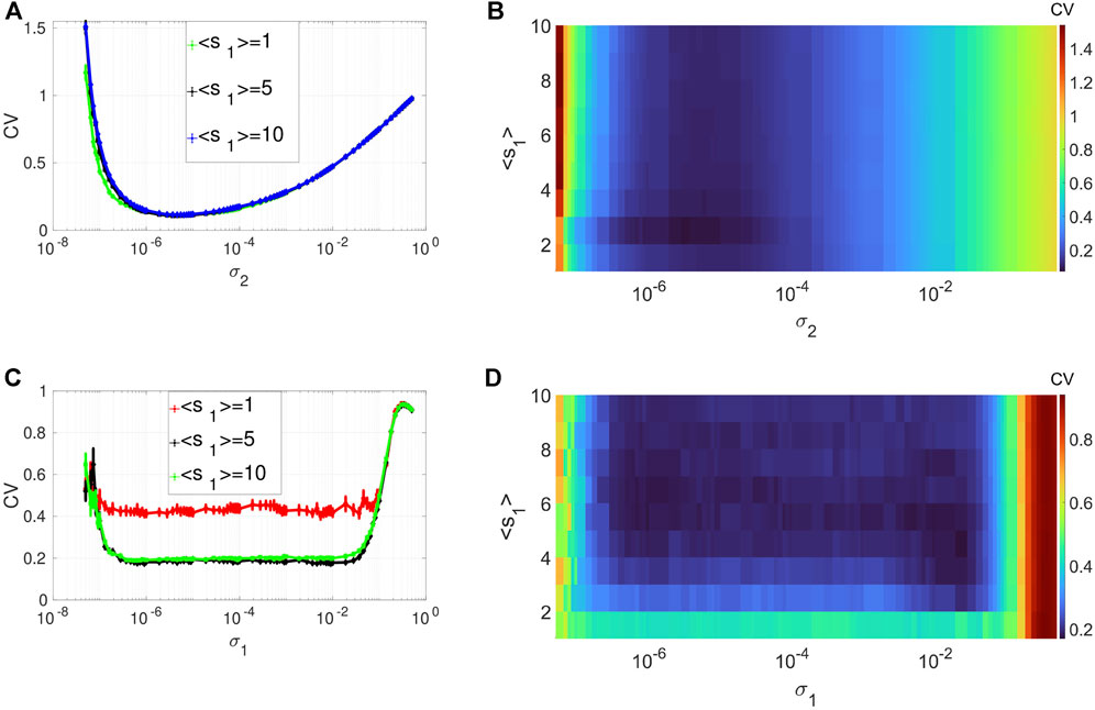
FIGURE 2. Variation of CV w.r.t. the average degree ⟨s₁⟩ and the noise intensity σ₂ for CR or σ₁ for SISR. Panels (A) and (B) show CR characterized by a family of non-monotonic CV curves w.r.t. σ₂ (σ₁ = 0) at ɛ₁ = 0.01. Panels (C) and (D) show SISR characterized by a family of non-monotonic CV curves w.r.t. σ₁ (σ₂ = 0) at ɛ₁ = 0.001. In both phenomena, the other parameters of the layer 1 are fixed at: β₁ = 0.1, τ₁ = 1, P₁ = 0.1, τ_1d = 20, D₁ = 0.5, τ_1p = 20, N = 50.

Figures 2C,D show the variation in the degree of SISR in layer 1 (in isolation) of Eq. 1. In this case, we switched on the synaptic noise intensity σ₁ (and turned off the channel noise, i.e., σ₂ = 0), decreased the timescale separation parameter from ɛ = 0.01 to ɛ = 0.001, and kept the rest of the parameters at the same values as in Figures 2A,B. In contrast to CR, SISR is sensitive to changes in the average degree parameter ⟨s₁⟩. In particular, when the network is very sparse, i.e., when ⟨s₁⟩ = 1, the degree of SISR becomes significantly lower, with a minimum value of the CV curve around CV_min = 0.4 for a wide range of the noise intensity, i.e., σ₁ ∈ (3.7 × 10^–7; 1.9, ×, 10^–2). As the network becomes denser, i.e., ⟨s₁⟩ increases, the degree of SISR also increases with the minimum value of the CV curves occurring at CV_min ≈ 0.1903 for σ₁ ∈ (3.7 × 10^–7; 1.9, ×, 10^–2). Thus, in the rest of our simulations, to have a high (low) degree of SISR, we will fix the average degree of the layer networks at ⟨s₁⟩ = 10 (⟨s₁⟩ = 1), in contrast to CR.

Interestingly, in Figure 2, we see that the best degree of coherence is higher for CR (with CV_min = 0.1108) than for SISR (with (CV_min ≈ 0.1903). In previous work [50], where we investigated CR and SISR in one isolated layer of Eq. 1 in the absence of STDP, the opposite behavior occurs, i.e., SISR produces a higher degree of coherence (with CV_min = 0.012) than CR (with CV_min = 0.130), when all the other parameters are at their optimal values. This means that in the presence (absence) of STDP, the degree of coherence due to CR (SISR) is higher than that of SISR (CR). Furthermore, while the degree of CR is higher than that of SISR, the range of values of the noise intensity in which the degree of CR is high is significantly smaller than that of SISR. This is explained by the fact that high coherence due to SISR emerges due to the asymptotic matching of the deterministic and stochastic timescales. While the high coherence due to CR emerges as a result of the proximity to the Hopf bifurcation [10, 50]. Figures 2C,D indicate that this matching of timescales occurs for a wider range of values of the synaptic noise intensity (with flat-bottom CV curves), hence the larger interval for coherence. On the other hand, Figures 2A,B show a smaller interval of the channel noise intensity in which the degree CR is highest. In this case, the noise intensity has to be just right (not too weak or strong) to let the systems oscillate between the excitable and the oscillatory regimes via a noise-induced Hopf bifurcation, leading to the emergence of a limit cycle behavior (i.e., noise-induced coherent oscillations). The noise channel noise should not be too weak so that the systems do not stay for too long in the excitable regime, thereby destroying the coherence. Nor should it be too strong to overwhelm the entire oscillations in the oscillatory regime, hence the relatively smaller noise interval for the highest coherence in the case of CR.

Figures 3A,B depict the variation in the degree of CR in layer 1 (in isolation) of Eq. 1 as a function of the channel noise intensity σ₂ and the network rewiring probability β₁ at an optimal value of the average degree (i.e., ⟨s₁⟩ = 1) chosen from Figure 2A. The other parameters are kept fixed at the values given in Figure 2. From Figures 3A,B, we notice that variations in the rewiring probability do not destroy the high degree of CR. Here the minimum of the CV curves remain very low. However, we can observe that when the network is regular, i. e, when β₁ = 0.0, the minimum of the CV curve (see, e.g., the green curve in Figure 3A) is noticeably lower than when we have small-world (with β₁ ∈ (0, 1)) and the random network (with β₁ = 1) topology. Nevertheless, because in this work we are interested in non-regular networks (i.e., β₁ ∈ (0, 1]), we will fix β₁ to a very low, but non-zero value (i.e., β₁ = 0.1) to have a high degree of CR in a small-world network. Hence, in the rest of our simulations, to have the best degree of CR in our small-world network, we will fix the rewiring probability of the layer networks at β₁ = 0.1.

FIGURE 3

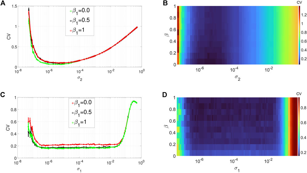
FIGURE 3. Variation of CV w.r.t. the wiring probability β₁ and the noise intensity σ₁ for SISR or σ₂ for CR. Panels (A) and (b) show the CV curves due to CR (σ₁ = 0, ɛ₁ = 0.01, ⟨s₁⟩ = 2). Panels (C) and (D) show the CV curves due to SISR (σ₂ = 0, ɛ₁ = 0.001, ⟨s₁⟩ = 10). In both phenomena, the other parameters are fixed at: τ₁ = 1, P₁ = 0.1, τ_1d = 20, D₁ = 0.5, τ_1p = 20, N = 50.

Figures 3C,D show the variation in the degree of SISR in layer 1 (in isolation) of Eq. 1 as a function of the synaptic noise intensity σ₁ and the network rewiring probability β₁ at the optimal value of the average degree (i.e., ⟨s₁⟩ = 10) chosen from Figure 2C. The rest of the parameter values are the same as in Figures 3A,B. We observe again that the degree of SISR is more sensitive to changes in the parameter β₁ than the degree of CR. Furthermore, we observe that varying the rewiring probability β₁ has the opposite effect on the degree of SISR compared to its effect on the degree of CR. The more regular the network is (see, e.g., the red curve in Figure 3C), the higher the CV curve and hence the lower the degree of SISR. Thus, in the rest of our simulations, to have the best degree of SISR in our network, we will fix the rewiring probability of the layer networks at β₁ = 1 (see the green curve in Figure 3C).

Figures 4A,B depict the variation in the degree of CR in layer 1 (in isolation) of Eq. 1 as a function of channel noise intensity σ₂ and the intra-layer time delay τ₁ of the network, at an optimal value of the average degree (i.e., ⟨s₁⟩ = 2) and the network rewiring probability (i.e., β₁ = 0.1) chosen from Figure 2A and Figure 3A, respectively. Again we notice, from the low values of the minimum of the CV curves, the robustness of the degree of CR to variations of a network parameter, i.e., τ₁. Nonetheless, with the low degree of CR, we can still observe that when the synaptic connections between the neurons are instantaneous (i.e., when τ₁ = 0), the CV curve (see the green curve in) is slightly lower than the rest of the curves. Further increase in the time delay does not affect the degree of CR. In the rest of the simulations, to have the best degree of CR in our network, we will fix the intra-layer time delay at a low but non-zero value, i.e., at τ₁ = 1.

FIGURE 4

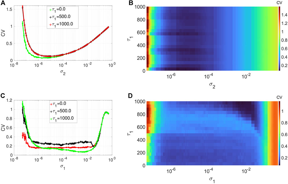
FIGURE 4. Variation of CV w.r.t. the time delay τ₁ and noise intensity σ₁ for SISR or σ₂ for CR. Panels (A) and (B) show the CV curves due to CR (σ₁ = 0, ɛ₁ = 0.01, ⟨s₁⟩ = 2). Panels (C) and (D) show the CV curves due to SISR (σ₂ = 0, ɛ₁ = 0.001, ⟨s₁⟩ = 10). In both phenomena, the other parameters are fixed at: τ₁ = 1, P₁ = 0.1, τ_1d = 20, D₁ = 0.5, τ_1p = 20, N = 50.

Figures 4C,D show the variation in the degree of SISR in layer 1 (in isolation) of Eq. 1 as a function of synaptic noise intensity σ₁ and the intra-layer time delay τ₁ at an optimal value of the average degree (i.e., ⟨s₁⟩ = 10) and the network rewiring probability (i.e., β₁ = 1) chosen from Figure 2C and Figure 3C, respectively. We observe that the degree of SISR is again more sensitive to parametric perturbations than the degree CR. Moreover, the variation in the degree of SISR as a function of the intra-layer time delay τ₁ is not linear and significantly depends on values of the synaptic noise σ₁. In Figure 4A, for τ₁ = 0.0, we have CV values which are higher and lower than those at τ₁ = 1,000 and τ₁ = 500, respectively. Thus, in the rest of the simulations, to have the best degree of SISR in our network, we will fix the intra-layer time delay at τ₁ = 1,000.

3.1.2 With respect to STDP Parameters: P₁, τ_1d

Using the insight from the previous section on the effects of each network parameter (i.e., ⟨s₁⟩, β₁, and τ₁) on the degree of CR and SISR, we now investigate the effects of STDP on the degree of CR and SISR by varying the parameters P₁ of the potentiation adjusting rate and τ_1d of the depression temporal window. To do this, we first note that the results in Figures 2–4 are obtained when the parameters of STDP (i.e., P₁ and τ_1d) are kept fixed at the values indicated in the captions. So in the sequel, we fix the network parameters at their non-optimal values, i.e., at values at which each phenomenon produces the lowest degree of coherence. Then, we vary the parameters (P₁ and τ_1d) of the STDP learning rule in layer 1.

Extensive numerical simulations (not shown) have indicated that the variations in the degree of CR and SISR with respect to P₁ and τ_1d are higher at the corresponding optimal network parameter values indicated in Figures 2–4 than at the non-optimal network parameter values. Qualitatively, however, the variations in the degrees of both phenomena are essentially the same when we have optimal or non-optimal network parameter values. Because we are interested in the highest degree of CR and SISR, we present the results on the effects of STDP on the degree of CR and SISR when the network parameters are non-optimal. We will then investigate the enhancement strategies of the degree of each phenomenon using the multiplexing technique.

In Figures 5A,B, we show the variations in degree of CR and SISR in layer 1 (in isolation) of Eq. 1 as a function of the channel (σ₂) and synaptic (σ₁) noise intensity and the potentiation adjusting rate parameter P₁ at corresponding non-optimal values of the network parameters, respectively. Figure 5A shows that the higher (compared to the degree of coherence induced by SISR in Figure 5B) degree of coherence induced CR is more (compared to the robustness of the coherence induced by SISR in Figure 5B) robust to variations in the potentiation adjusting rate parameter P₁. Even though the lowest CV values for each value of P₁ are relatively close to each other, we have the lowest (highest) CV_min = 0.1363 (CV_min = 0.1804) occurring at P₁ = 0.1 (P₁ = 1). For SISR, we the lowest (highest) CV_min = 0.2009 (CV_min = 0.2588) occurs at P₁ = 0.1 (P₁ = 1).

FIGURE 5

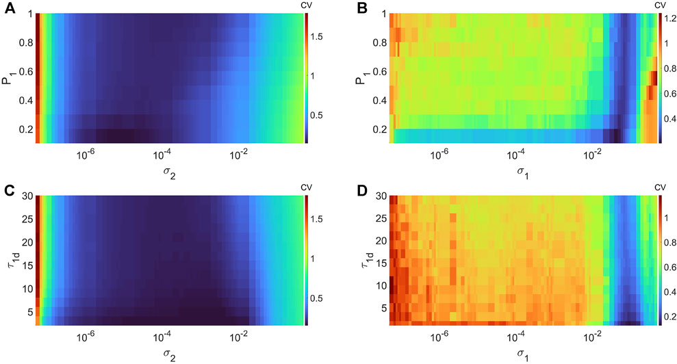
FIGURE 5. Variation of CV w.r.t. the potentiation adjusting rate P₁, depression temporal window τ_1d, and the noise intensity σ₁ or σ₂, with the corresponding non-optimal network parameter values. Panel (A) and (B) show the values of CV during CR (σ₁ = 0, ɛ₁ = 0.01, ⟨s₁⟩ = 10, β = 1, τ₁ = 100, τ_1d = 20) and during SISR (σ₂ = 0, ɛ₁ = 0.001, ⟨s₁⟩ = 1, β = 0.1 τ₁ = 600, τ_1d = 20). Panel (C) and (D) show the values CV during CR (σ₁ = 0, ɛ₁ = 0.01,⟨s₁⟩ = 10, β = 1, τ₁ = 100, P₁ = 1) and during SISR (σ₂ = 0, ɛ₁ = 0.001, ⟨s₁⟩ = 1, β = 0.1, τ₁ = 600, P₁ = 1). In both phenomena, the other parameters are fixed at: D₁ = 0.5, τ_1p = 20, N = 50.

In Figures 5C,D, we show the variations in degree of CR and SISR in layer 1 (in isolation) of Eq. 1 as a function of the channel (σ₂) and synaptic (σ₁) noise intensity and the depression temporal window τ_1d at corresponding non-optimal values both of the network parameters and the potentiation adjusting rate parameter P₁ (obtained from Figures 5A,B), respectively. For CR, we the lowest (highest) CV_min = 0.0254 (CV_min = 0.1849) occurs at τ_1d = 0.01 (τ_1d = 30). For SISR, we the lowest (highest) CV_min = 0.1245 (CV_min = 0.2632) occurs at τ_1d = 0.01 (τ_1d = 30). Thus, unlike the opposite effects of the variations in each network parameter on the degree of CR and SISR, the variations in the STDP parameters have similar effects on the degree of CR and SISR.

In previous work [50], we aimed at enhancing CR (and not SISR) via the multiplexing technique because CR showed more sensitivity to parametric perturbations than SISR in the absence of the STDP learning rule. The results in Figures 2–5 indicate that the degree of CR becomes more robust to parametric perturbations than the degree of SISR, which is particularly sensitive to the variations in the parameters of the STDP learning rule. For this reason, in the next section, we focus only on the enhancement of the more sensitive phenomenon, i.e., SISR, via the multiplexing technique used in [50].

3.2 Enhancement of SISR via the Multiplexing Technique

It has been shown in [50] that in a two-layer multiplex network with static (non-adaptive) synaptic couplings, CR or SISR in one layer could induce and enhance CR in the other layer. Here, we address whether enhancing a low degree of SISR in one layer of a multiplex network is possible using an enhanced CR or SISR in the other layer when adaptive synaptic couplings drive the network. Then, we investigate which enhancement scheme is best: 1) the CR-SISR scheme or 2) the SISR-SISR scheme.

In the CR-SISR scheme, we use the results from Section 3.1 and we set layer 1 such that it has a low degree of SISR, i.e., we choose the network and STDP parameter values (⟨s₁⟩ = 1, β₁ = 0.1, τ₁ = 600, P₁ = 1, τ_1d = 0.01) so that the CV curve is high—indicating a poor degree of SISR in layer 1 in isolation. We also set layer two such that it has a high degree of CR, i.e., we choose the network and the STDP parameter values (⟨s₁⟩ = 2, β₂ = 0.1, τ₂ = 1, P₂ = 0.1, τ_2d = 20) so that the CV curve is low—indicating a high degree of CR in layer 2 in isolation. Then, we couple the two layers in a multiplex fashion, i.e., each neuron in a layer is coupled only to its replica neuron in the other layer via a synaptic coupling driven by STDP. In the SISR-SISR scheme, we have the same settings as in the CR-SISR scheme, except that in layer 2, we set the network and STDP parameter values (⟨s₂⟩ = 10, β₂ = 1, τ₂ = 1, P₂ = 0.1, τ_2d = 20) so that the CV curve is high—in indicating a high degree of SISR in layer 2 in isolation.

The STDP driving the multiplexing (inter-layer) synaptic connections is governed by synaptic weight $K_{ii}^{12}(t)$ that evolves according Eqs. 4, 5. Similarly to the intra-layer synaptic weights of the isolated layer networks of Section 3.1, we will fix the depression adjusting rate parameter at D₁₂ = 0.5 and the potentiation temporal window parameter at τ_12p = 20, and vary only the potentiation adjusting rate P₁₂ ∈ [0.05, 1], the depression temporal window τ_12d ∈ [0.2, 30], and the inter-layer time delay τ₁₂ ∈ [0.0, 1,000] parameters in the intervals indicated.

In Figure 6, we show the performance of each scheme in enhancing the low degree of SISR in layer 1. Figures 6A,B depict the performances for an instantaneous (i.e., τ₁₂ = 0) multiplexing and for a time-delayed (τ₁₂ = 1,000) multiplexing between layer 1 and layer 2, respectively. We recall that layer 1 is the layer of interest, i.e., the layer with a low degree of SISR when it is in isolation. The red curve in Figures 6A,B represents the degree of coherence due to SISR in layer 1 when it is in isolation. We can see that for the selected set of network and STDP parameters (i.e. ⟨s₁⟩ = 1, β₁ = 0.1, τ₁ = 600, P₁ = 1, τ_1d = 0.01), the degree of coherence due to SISR is very low as indicated by the high values of the red CV curve for values of the synaptic noise intensity in some interval, i.e., σ₁ ∈ (5.0, ×, 10^–8, 3.5 × 10^–2).

FIGURE 6

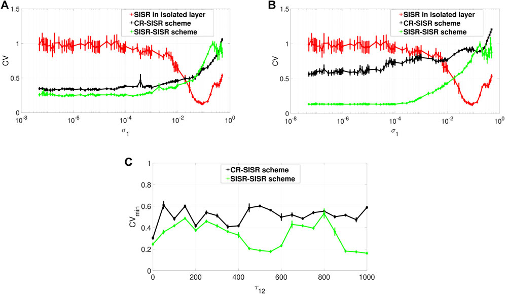
FIGURE 6. Variation of CV of the controlled layer (exhibiting SISR) w.r.t. the noise intensity σ₁ and the inter-layer time delay τ₁₂. Panels (A) and (B) show the CV curves in the absence (τ₁₂ = 0) and presence (τ₁₂ = 1,000) of the inter-layer time delay τ₁₂, respectively. The red curves represent the variation in the degree of SISR in layer 1 when in isolation. The black and the green curves show the enhancement performances of the CR-SISR and SISR-SISR schemes, respectively. Panel (C) shows that for the same value of the inter-layer time delay, the SISR-SISR scheme always outperforms the CR-SISR scheme. Parameters of layer 2 in the CR-SISR scheme: ${\widehat{\sigma }}_1={\sigma }_2=0$, ${\widehat{\sigma }}_2={\sigma }_1\ne 0$, ɛ₂ = 0.01, ⟨s₂⟩ = 2, β₂ = 0.1, τ₂ = 1, P₂ = 0.1, τ_2d = 20. Parameters of layer 2 in the SISR-SISR scheme: ${\widehat{\sigma }}_2={\sigma }_2=0$, ${\widehat{\sigma }}_1={\sigma }_1\ne 0$, ɛ₂ = 0.001, ⟨s₂⟩ = 10, β₂ = 1, τ₂ = 1, P₂ = 0.1, τ_2d = 20. Parameters of layer 1 in isolation and in both schemes: ɛ₁ = 0.001, ⟨s₁⟩ = 1, β₁ = 0.1, τ₁ = 600, P₁ = 1, τ_1d = 0.01, N = 50. Parameters of the inter-layer STDP: P₁₂ = 1, τ_12d = 30, D₁₂ = 0.5, τ_12p = 20.

When layer 1, with its poor degree of SISR, is multiplexed with layer 2 exhibiting a high degree of CR, the performance of this CR-SISR scheme is depicted by the black curve in Figures 6A,B which represent the new degree of SISR in layer 1. We see that the multiplexing of layer 1 with another layer exhibiting a strong CR can significantly improve the degree of SISR in layer 1 by lowering the red CV curve, which becomes black. On the other hand, when layer 1, with its poor degree of SISR, is multiplexed with layer 2 exhibiting a high degree of SISR, the performance of this SISR-SISR scheme is depicted by the green curve in Figures 6A,B which represent the new degree of SISR in layer 1. We see that the multiplexing of layer 1 with another layer exhibiting a strong SISR can significantly improve the degree of SISR in layer 1 by lowering the red CV curve, which becomes green. However, in both schemes, this enhancement of SISR in layer 1 fails when the synaptic noise intensity is larger than 1.9 × 10^–2, a point from which the black and the green CV curves of the CR-SISR and SISR-SISR schemes lie above the red CV curve of layer 1 in isolation.

Furthermore, we observe that even though the degree of the coherence induced by CR can be higher than the degree of coherence induced by SISR in an isolated layer network driven by STDP, the degree of SISR induced via a multiplexing SISR-SISR enhancement scheme is higher than that induced by a CR-SISR enhancement scheme. This is clearly indicated by the black and green curves simulated with no inter-layer time delay in Figure 6A and with an inter-layer time delay in Figure 6B. For the majority of values of the synaptic noise intensity of layer 1, the green curve lies entirely below the black one.

To further investigate the effect of the inter-layer time delay τ₁₂ on the degree of coherence due to SISR in layer 1, we computed the minimum value of the CV curve, (i.e., CV_min) for a wide range of values of the inter-layer time delay τ₁₂. The result is shown in Figure 6C, where the green curve representing the enhancement performance of the SISR-SISR scheme always lies below the black curve, which represents the performance of the CR-SISR scheme, as the inter-layer time delay changes in τ₁₂ ∈ [0, 1,000]. Figure 6C also indicates that when the inter-layer time delay is at τ₁₂ = 550 and τ₁₂ = 1,000, the SISR-SISR scheme performs significantly better than at other values of the inter-layer time delay and the CR-SISR scheme. The best inter-layer time delay values in the CR-SISR scheme occur at τ₁₂ = 0 and at τ₁₂ = 350. The results presented in Figure 6 are for fixed values of the alterable parameters of the inter-layer STDP learning rule, i.e. P₁₂ = 0.05 and τ_12d = 30.

Now we investigate the effects of varying these two parameters on the performances of the CR-SISR and SISR-SISR enhancement schemes. To implement this, we fix, from Figure 6C, the inter-layer time delay at the optimal value for each scheme, i.e., τ₁₂ = 350 and τ₁₂ = 1,000 for the CR-SISR and the SISR-SISR scheme, respectively. Figures 7A,B show the performances of the CR-SISR and SISR-SISR schemes as a function of the multiplexing STDP parameters, i.e., P₁₂ and τ_12d, respectively. For the CR-SISR scheme, we observe that a larger depression temporal window (i.e., τ_12d → 30) and a smaller potentiation adjusting rate (P₁₂ → 0.05) yield the lowest minimum CV value, given by CV_min = 0.2989 which occurs at the synaptic noise intensity of ${\sigma }_1=1.9,\times ,10^{-4}={\widehat{\sigma }}_2$.

FIGURE 7

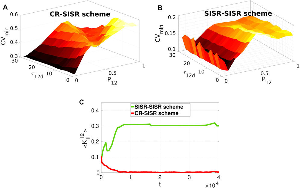
FIGURE 7. Minimum CV against the multiplexing potentiation adjusting rate P₁₂ and depression temporal window τ_12d for layer 1 exhibiting SISR when multiplexed to layer 2 exhibiting CR and SISR in Panels (A) and (B), respectively. The SISR-SISR scheme outperforms the CR-SISR scheme in enhancing SISR in layer 1 in the entire (τ_12d, P₁₂) plane. Parameter values in panels (A) and (B) are the same as in (Figure 6A) with τ₁₂ = 350 and τ₁₂ = 1,000 in the CR-SISR and SISR-SISR scheme, respectively. Panel (C) shows the time-evolution of population-averaged inter-layer synaptic weights $⟨K_{ii}^{12}⟩$ with an initial normal distribution of mean 0.1 and standard deviation 0.02 at the values of P₁₂, τ_12d, and σ₁ (see main text) at which CV_min achieves it lowest value in CR-SISR and the SISR-SISR schemes. LTP (LTD) favours the SISR-SISR scheme (CR-SISR scheme).

The SISR-SISR scheme in Figure 7B shows better overall performance compared to the CR-SISR scheme with respect to these inter-layer STDP parameters. First, we observe that the surface of the graph CV_min in the SISR-SISR scheme (with the highest value at CV_min = 0.2098, occurring at P₁₂ = 0.5 and τ₁₂ = 0.5) lies entirely below the surface of the graph CV_min in the CR-SISR scheme (with the lowest value at CV_min = 0.2989, occurring at P₁₂ = 0.05 and τ_12d = 30). Secondly, from Figure 7B, we observe that small (i.e., P₁₂ = 0.1), but not too small values (unlike in the CR-SISR scheme in Figure 7A with P₁₂ = 0.05) of the potentiation adjusting rate and large values of the depression temporal window (i.e., τ₁₂ = 30) parameters yield the lowest minimum CV value, given by CV_min = 0.1005 which occurs at the synaptic noise intensity of ${\sigma }_1=7.3\times 10^{-5}={\widehat{\sigma }}_1$.

In [50], the synaptic connections between the FHN neurons are static, and the effects of STDP on the strength of synaptic couplings are entirely ignored. The results [50] show that intermediate and strong multiplexing between the layer networks is required for the enhancement of the coherence, irrespective of the enhancement scheme. However, in the current paper, the inter-layer synaptic strength may not be static. Thus, we cannot choose a priori the strength of the inter-layer synaptic connections because this is entirely controlled by the STDP rule, which depends on the neurons’ random spiking times. The best performance of the CR-SISR scheme (indicated by the lowest of value of CV_min in Figure 7A) occurs when P₁₂ = 0.05, τ_12d = 30, τ₁₂ = 350, and σ₁ = 1.9, ×, 10^–4. While the best performance of the SISR-SISR scheme (indicated by the lowest value CV_min in Figure 7B) occurs when P₁₂ = 0.1, τ_12d = 30, τ₁₂ = 1,000, and σ₁ = 7.3 × 10^–5. Now, using these two sets of parameter values, we computed the time-evolution of the population-averaged multiplexing synaptic weights $⟨K_{ii}^{12}⟩$ with an initial normal distribution of mean 0.1 and standard deviation of 0.02. The results are depicted in Figure 7C where the green curve shows that the best enhancement of SISR via the SISR-SISR scheme occurs via LTP, i.e., the strengthening of the inter-layer synapses from the initial value. In contrast, the red curve shows that the best enhancement of SISR via the CR-SISR scheme occurs via LTD, i.e., the weakening of the inter-layer synapses from the initial value. We note that the red curve in Figure 7C is close to zero, but not exactly zero (since the elimination of synapses has been avoided by bounding $⟨K_{ii}^{12}⟩\in [0.0001,1]$). The fact that the weak multiplexing of layer networks could enhance resonance phenomena in one of the layers was already discovered in [39]. However, this remains an observed behavior as the precise mechanism behind it is still elusive. A theoretical explanation of weak-multiplexing-induced resonance phenomena should be rewarding in theoretical studies and applications, e.g., in neuroengineering.

4 Summary and Conclusion

In this paper, we have numerically investigated the effects of varying the network and STDP parameters on the degree of CR and SISR in isolated and coupled (multiplexed) layer networks consisting of electrically connected FHN model neurons. In the isolated layer networks and for a fixed set of parameters, the results indicate that: 1) in the presence of STDP, the degree and the robustness of the coherence due to CR are always higher than those of the coherence due to SISR, unlike in the absence of STDP where the opposite behaviors occur [50], 2) the degree of coherence due to SISR increases with the average degree of the network connectivity and the rewiring probability of the network topology. While the degree of the coherence due to SISR shows a nonlinear response to the variation in the electric time delay between the neurons—smaller and significantly larger time delays yield a higher degree of coherence than intermediate values, and 3) the degree of coherence due to SISR increases with a decreasing (increasing) value of the depression temporal window (potentiation adjusting rate) parameter of the STDP learning rule, especially at (relatively) larger synaptic noise intensities.

In the multiplex networks, we set up two enhancement schemes for the more sensitive phenomenon, i.e., SISR in layer 1, based on the multiplexing with layer 2 and using SISR and CR acting as the enhancing phenomena each with a high degree of coherence in layer 2. In the first enhancement scheme (termed the CR-SISR scheme), we have SISR with a low degree of coherence, achieved with specific values of the network and STDP parameter in layer 1 obtained in advance. And in layer 2 we have CR with a high degree of coherence, achieved with specific values of the network and STDP parameters obtained in advance. In the second enhancement scheme, termed the SISR-SISR scheme, we have SISR with a low degree of coherence in layer 1. And in layer 2 we have SISR with a high degree of coherence. Our results showed that: 1) both schemes can significantly enhance (as indicated by the relatively lower value of the CV curves) the poor degree of SISR in layer 1, 2) at the optimal inter-layer time delay (τ₁₂) of each scheme, a larger depression temporal window (τ_12d) and a smaller potentiation adjusting rate (P₁₂) parameters of the inter-layer STDP learning rule improve the CR-SISR and SISR-SISR enhancement schemes. However, for the SISR-SISR scheme, the potentiation adjusting rate parameter should not be too small, 3) the SISR-SISR scheme outperforms the CR-SISR scheme in the enhancement of SISR in layer 1 for all the parameter values of the inter-layer STDP learning rule, and 4) at their respective optimal inter-layer time delay, synaptic noise intensity, potentiation adjusting rate, and depression temporal window parameter values, the SISR-SISR scheme enhances SISR in layer 1 via long-term potentiation (LTP) of the synaptic strength between the layers. In contrast, the CR-SISR scheme enhances SISR in layer 1 via long-term depression (LTD) of the synaptic strength between the layers.

Interesting future research directions on the topic would be to investigate the robustness of the results presented in this paper when the topologies of the layer and multiplex networks are different and when the networks are driven by homeostatic structural plasticity.

Data Availability Statement

The original contributions presented in the study are included in the article/Supplementary Material, further inquiries can be directed to the corresponding author.

Author Contributions

MY designed the study, conducted the numerical simulations, analyzed the results, and wrote the manuscript. TT analyzed the results and wrote the manuscript. JJ analyzed the results and wrote the manuscript. All the authors have approved the submitted version.

Conflict of Interest

The authors declare that the research was conducted in the absence of any commercial or financial relationships that could be construed as a potential conflict of interest.

Publisher’s Note

All claims expressed in this article are solely those of the authors and do not necessarily represent those of their affiliated organizations, or those of the publisher, the editors and the reviewers. Any product that may be evaluated in this article, or claim that may be made by its manufacturer, is not guaranteed or endorsed by the publisher.

Acknowledgments

MY acknowledges support from the Deutsche Forschungsgemeinschaft (DFG, German Research Foundation)—Project No. 456989199.

References

1. Aust R, Hövel P, Hizanidis J, Schöll E .Delay Control of Coherence Resonance in Type-I Excitable Dynamics. Eur Phys J Spec Top (2010) 187:77–85. doi:10.1140/epjst/e2010-01272-5

CrossRef Full Text | Google Scholar

2. Bačić I, Klinshov V, Nekorkin V, Perc M, Franović I .Inverse Stochastic Resonance in a System of Excitable Active Rotators with Adaptive Coupling. EPL (Europhysics Letters) (2018) 124:40004.

Google Scholar

3. Benzi R, Sutera A, Vulpiani A .The Mechanism of Stochastic Resonance. J Phys A: Math Gen (1981) 14:L453–L457. doi:10.1088/0305-4470/14/11/006

CrossRef Full Text | Google Scholar

4. Bi G-q., Poo M-m. .Synaptic Modifications in Cultured Hippocampal Neurons: Dependence on Spike Timing, Synaptic Strength, and Postsynaptic Cell Type. J Neurosci (1998) 18:10464–72. doi:10.1523/jneurosci.18-24-10464.1998

PubMed Abstract | CrossRef Full Text | Google Scholar

5. Bianconi GMultilayer Networks: Structure and Function. Oxford University Press (2018).

Google Scholar

6. Bönsel F, Krauss P, Metzner C, Yamakou ME .Control of Noise-Induced Coherent Oscillations in Three-Neuron Motifs. Cogn Neurodynamics (2021) 1–20. doi:10.1007/s11571-021-09770-2

CrossRef Full Text | Google Scholar

7. Dan Y, Poo M-M .Spike Timing-dependent Plasticity: from Synapse to Perception. Physiol Rev (2006) 86:1033–48. doi:10.1152/physrev.00030.2005

PubMed Abstract | CrossRef Full Text | Google Scholar

8. De Domenico M .Multilayer Modeling and Analysis of Human Brain Networks. Gigascience (2017) 6:1–8. doi:10.1093/gigascience/gix004

PubMed Abstract | CrossRef Full Text | Google Scholar

9. Debanne D, Gähwiler BH, Thompson SM .Long-term Synaptic Plasticity between Pairs of Individual Ca3 Pyramidal Cells in Rat Hippocampal Slice Cultures. J Physiol (1998) 507:237–47. doi:10.1111/j.1469-7793.1998.237bu.x

PubMed Abstract | CrossRef Full Text | Google Scholar

10. DeVille RE, Vanden-Eijnden E, Muratov CB .Two Distinct Mechanisms of Coherence in Randomly Perturbed Dynamical Systems. Phys Rev E Stat Nonlin Soft Matter Phys (2005) 72:031105. doi:10.1103/PhysRevE.72.031105

PubMed Abstract | CrossRef Full Text | Google Scholar

11. FitzHugh R .Mathematical Models of Threshold Phenomena in the Nerve Membrane. Bull Math Biophys (1955) 17:257–78. doi:10.1007/bf02477753

CrossRef Full Text | Google Scholar

12. Franović I, Yanchuk S, Eydam S, Bačić I, Wolfrum M .Dynamics of a Stochastic Excitable System with Slowly Adapting Feedback. Chaos: Interdiscip J Nonlinear Sci (2020) 30:083109.

Google Scholar

13. Friederici AD, Singer W .Grounding Language Processing on Basic Neurophysiological Principles. Trends Cognitive Sciences (2015) 19:329–38. doi:10.1016/j.tics.2015.03.012

PubMed Abstract | CrossRef Full Text | Google Scholar

14. Froemke RC, Dan Y .Spike-timing-dependent Synaptic Modification Induced by Natural Spike Trains. Nature (2002) 416:433–8. doi:10.1038/416433a

PubMed Abstract | CrossRef Full Text | Google Scholar

15. Geffert PM, Zakharova A, Vüllings A, Just W, Schöll E .Modulating Coherence Resonance in Non-excitable Systems by Time-Delayed Feedback. Eur Phys J B (2014) 87:291. doi:10.1140/epjb/e2014-50541-2

CrossRef Full Text | Google Scholar

16. Gerstner W, Kempter R, Van Hemmen JL, Wagner H .A Neuronal Learning Rule for Sub-millisecond Temporal Coding. Nature (1996) 383:76–8. doi:10.1038/383076a0

PubMed Abstract | CrossRef Full Text | Google Scholar

17. Gu H, Zhang H, Wei C, Yang M, Liu Z, Ren W .Coherence Resonance-Induced Stochastic Neural Firing at a Saddle-Node Bifurcation. Int J Mod Phys B (2011) 25:3977–86. doi:10.1142/s0217979211101673

CrossRef Full Text | Google Scholar

18. Gutkin BS, Jost J, Tuckwell HC .Inhibition of Rhythmic Neural Spiking by Noise: the Occurrence of a Minimum in Activity with Increasing Noise. Naturwissenschaften (2009) 96:1091–7. doi:10.1007/s00114-009-0570-5

PubMed Abstract | CrossRef Full Text | Google Scholar

19. Hizanidis J, Schöll E .Control of Coherence Resonance in Semiconductor Superlattices. Phys Rev E Stat Nonlin Soft Matter Phys (2008) 78:066205. doi:10.1103/PhysRevE.78.066205

PubMed Abstract | CrossRef Full Text | Google Scholar

20. Jia B, Gu H-G, Li Y-Y .Coherence-resonance-induced Neuronal Firing Near a Saddle-Node and Homoclinic Bifurcation Corresponding to Type-I Excitability. Chin Phys. Lett. (2011) 28:090507. doi:10.1088/0256-307x/28/9/090507

CrossRef Full Text | Google Scholar

21. Kasdin NJ .Runge-kutta Algorithm for the Numerical Integration of Stochastic Differential Equations. J Guidance, Control Dyn (1995) 18:114–20. doi:10.2514/3.56665

CrossRef Full Text | Google Scholar

22. Kim S-Y, Lim W .Stochastic Spike Synchronization in a Small-World Neural Network with Spike-timing-dependent Plasticity. Neural Networks (2018) 97:92–106. doi:10.1016/j.neunet.2017.09.016

PubMed Abstract | CrossRef Full Text | Google Scholar

23. Knuth DEThe Art of Computer Programming, 2. Reading, MA: Addison-Wesley (1973). p. 51.

Google Scholar

24. Kuehn CMultiple Time Scale Dynamics, 191. Springer (2015).

Google Scholar

25. Lindner B, Garcıa-Ojalvo J, Neiman A, Schimansky-Geier L .Effects of Noise in Excitable Systems. Phys Rep (2004) 392:321–424. doi:10.1016/j.physrep.2003.10.015

CrossRef Full Text | Google Scholar

26. Lindner B, Schimansky-Geier L .Analytical Approach to the Stochastic Fitzhugh-Nagumo System and Coherence Resonance. Phys Rev E (1999) 60:7270–6. doi:10.1103/physreve.60.7270

CrossRef Full Text | Google Scholar

27. Liu Z-Q, Zhang H-M, Li Y-Y, Hua C-C, Gu H-G, Ren W .Multiple Spatial Coherence Resonance Induced by the Stochastic Signal in Neuronal Networks Near a Saddle-Node Bifurcation. Physica A: Stat Mech its Appl (2010) 389:2642–53. doi:10.1016/j.physa.2010.02.029

CrossRef Full Text | Google Scholar

28. Longtin A .Stochastic Resonance in Neuron Models. J Stat Phys (1993) 70:309–27. doi:10.1007/bf01053970

CrossRef Full Text | Google Scholar

29. Markram H, Lübke J, Frotscher M, Sakmann B .Regulation of Synaptic Efficacy by Coincidence of Postsynaptic Aps and Epsps. Science (1997) 275:213–5. doi:10.1126/science.275.5297.213

PubMed Abstract | CrossRef Full Text | Google Scholar

30. Masoliver M, Malik N, Schöll E, Zakharova A .Coherence Resonance in a Network of Fitzhugh-Nagumo Systems: Interplay of Noise, Time-Delay, and Topology. Chaos (2017) 27:101102. doi:10.1063/1.5003237

PubMed Abstract | CrossRef Full Text | Google Scholar

31. Masoliver M, Masoller C, Zakharova A .Control of Coherence Resonance in Multiplex Neural Networks. Chaos, Solitons & Fractals (2021) 145:110666. doi:10.1016/j.chaos.2021.110666

CrossRef Full Text | Google Scholar

32. Masquelier T, Guyonneau R, Thorpe SJ .Spike Timing Dependent Plasticity Finds the Start of Repeating Patterns in Continuous Spike Trains. PloS one (2008) 3:e1377. doi:10.1371/journal.pone.0001377

PubMed Abstract | CrossRef Full Text | Google Scholar

33. Morrison A, Aertsen A, Diesmann M .Spike-timing-dependent Plasticity in Balanced Random Networks. Neural Comput (2007) 19:1437–67. doi:10.1162/neco.2007.19.6.1437

PubMed Abstract | CrossRef Full Text | Google Scholar

34. Muratov CB, Vanden-Eijnden E, E. W .Self-induced Stochastic Resonance in Excitable Systems. Physica D: Nonlinear Phenomena (2005) 210:227–40. doi:10.1016/j.physd.2005.07.014

CrossRef Full Text | Google Scholar

35. Pei X, Wilkens L, Moss F .Noise-mediated Spike Timing Precision from Aperiodic Stimuli in an Array of hodgekin-huxley-type Neurons. Phys Rev Lett (1996) 77:4679–82. doi:10.1103/physrevlett.77.4679

PubMed Abstract | CrossRef Full Text | Google Scholar

36. Pikovsky AS, Kurths J .Coherence Resonance in a Noise-Driven Excitable System. Phys Rev Lett (1997) 78:775–8. doi:10.1103/physrevlett.78.775

CrossRef Full Text | Google Scholar

37. Ren Q, Kolwankar KM, Samal A, Jost J .Hopf Bifurcation in the Evolution of Networks Driven by Spike-timing-dependent Plasticity. Phys Rev E Stat Nonlin Soft Matter Phys (2012) 86:056103. doi:10.1103/PhysRevE.86.056103

PubMed Abstract | CrossRef Full Text | Google Scholar

38. Semenov V, Feoktistov A, Vadivasova T, Schöll E, Zakharova A .Time-delayed Feedback Control of Coherence Resonance Near Subcritical Hopf Bifurcation: Theory versus experiment. Chaos (2015) 25:033111. doi:10.1063/1.4915066

PubMed Abstract | CrossRef Full Text | Google Scholar

39. Semenova N, Zakharova A .Weak Multiplexing Induces Coherence Resonance. Chaos (2018) 28:051104. doi:10.1063/1.5037584

PubMed Abstract | CrossRef Full Text | Google Scholar

40. Shepherd GMThe Synaptic Organization of the Brain. Oxford University Press (2004).

Google Scholar

41. Strogatz SH .Exploring Complex Networks. nature (2001) 410:268–76. doi:10.1038/35065725

PubMed Abstract | CrossRef Full Text | Google Scholar

42. Tuckwell HC, Jost J, Gutkin BS .Inhibition and Modulation of Rhythmic Neuronal Spiking by Noise. Phys Rev E Stat Nonlin Soft Matter Phys (2009) 80:031907. doi:10.1103/PhysRevE.80.031907

PubMed Abstract | CrossRef Full Text | Google Scholar

43. Watts DJSmall Worlds: The Dynamics of Networks between Order and Randomness. Princeton University Press Princeton (2000).

Google Scholar

44. Watts DJ, Strogatz SH .Collective Dynamics of 'small-World' Networks. nature (1998) 393:440–2. doi:10.1038/30918

PubMed Abstract | CrossRef Full Text | Google Scholar

45. Wolters A, Sandbrink F, Schlottmann A, Kunesch E, Stefan K, Cohen LG, et al. A Temporally Asymmetric Hebbian Rule Governing Plasticity in the Human Motor Cortex. J Neurophysiol (2003) 89:2339–45. doi:10.1152/jn.00900.2002

PubMed Abstract | CrossRef Full Text | Google Scholar

46. Yamakou ME, Hjorth PG, Martens EA .Optimal Self-Induced Stochastic Resonance in Multiplex Neural Networks: Electrical vs. Chemical Synapses. Front Comput Neurosci (2020) 14:62. doi:10.3389/fncom.2020.00062

PubMed Abstract | CrossRef Full Text | Google Scholar

47. Yamakou ME, Inack EM(2022). Coherence Resonance and Stochastic Synchronization in a Small-World Neural Network: An Interplay in the Presence of Spike-timing-dependent Plasticity. arXiv preprint arXiv:2201.05436.

Google Scholar

48. Yamakou ME, Jost J .A Simple Parameter Can Switch between Different Weak-Noise-Induced Phenomena in a Simple Neuron Model. Epl (2017) 120:18002. doi:10.1209/0295-5075/120/18002

CrossRef Full Text | Google Scholar

49. Yamakou ME, Jost J .Weak-noise-induced Transitions with Inhibition and Modulation of Neural Oscillations. Biol Cybern (2018) 112:445–63. doi:10.1007/s00422-018-0770-1

PubMed Abstract | CrossRef Full Text | Google Scholar

50. Yamakou ME, Jost J .Control of Coherence Resonance by Self-Induced Stochastic Resonance in a Multiplex Neural Network. Phys Rev E (2019) 100:022313. doi:10.1103/PhysRevE.100.022313

PubMed Abstract | CrossRef Full Text | Google Scholar

51. Zamani A, Novikov N, Gutkin B .Concomitance of Inverse Stochastic Resonance and Stochastic Resonance in a Minimal Bistable Spiking Neural Circuit. Commun Nonlinear Sci Numer Simulation (2020) 82:105024. doi:10.1016/j.cnsns.2019.105024

CrossRef Full Text | Google Scholar

52. Zhang LI, Tao HW, Holt CE, Harris WA, Poo M-m. .A Critical Window for Cooperation and Competition Among Developing Retinotectal Synapses. Nature (1998) 395:37–44. doi:10.1038/25665

PubMed Abstract | CrossRef Full Text | Google Scholar