Finite-Size Scaling on a Digital Quantum Simulator Using Quantum Restricted Boltzmann Machine

1 Introduction

A phase transition occurs whenever the thermodynamic functions of a system become non-analytic e.g. as a liquid changes into a gas, the density of the system changes discontinuously. If the phase transition occurs at a finite temperature T ≠ 0, the transition is called a classical phase transition (CPT) as it is dominated by thermal fluctuations. On the other hand, if the transition occurs by tuning some parameter in the system’s Hamiltonian as T → 0, it is called a quantum phase transition (QPT) since it is dominated by quantum fluctuations. A CPT appears only when the system is infinite i.e., in the thermodynamic limit [1]. On the other hand, a QPT doesn’t necessarily require the thermodynamic limit. Recently there has been a lot of interest in QPTs occurring in finite size light-matter interaction systems [2–7].

Quantum Rabi Model (QRM) describes the interaction of a two-level system with a bosonic field mode (see Eq. 1 for the Hamiltonian.) This model has gained a lot of significance in the study of ultrastrong light-matter coupling regimes where the so-called counterrotating terms can not be ignored [8]. Quantum Rabi Model has been shown to exhibit a QPT [2]. Namely, when the energy separation of the two levels in the system Ω becomes infinitely large compared to the frequency of the bosonic mode ω₀, the ground state of the Hamiltonian undergoes a phase transition from a normal phase to a superradiant phase as the light-matter coupling exceeds the critical value. Moreover, the ground state of the Jaynes-Cummings model (JCM) which can be obtained from the QRM by performing the rotating-wave approximation has also been shown to exhibit the normal-superradiant phase transition [3]. Later on, a more general anisotropic QRM in which the rotating and counter-rotating terms can have different coupling strengths was also considered [4]. The QRM and JCM are limiting cases of this model. It was shown that the ground state for this more general case also undergoes the normal-superradiant phase transition. The phase transition in QRM has also been demonstrated experimentally using a ¹⁷¹Yb⁺ ion in a Paul trap [7]. This experimental demonstration of a phase transition in a single two-level system has incited a lot of interest since this opens up an avenue for studying critical phenomena in controlled, small quantum systems.

In CPTs and some QPTs (which require N → ∞), a finite-size scaling (FSS) analysis can be done to extract the critical point and the critical exponents of the transition [1, 9]. While this procedure is inapplicable to the QPTs discussed above since these phase transitions occur at a finite system size, the phase transitions in these paradigmatic light-matter interaction models occur only in the limit Ω/ω₀ → ∞ and FSS analysis can be done in Ω/ω₀ [2–4] instead. In this paper, however, we propose a different approach to study such phase transitions. We apply the FSS in Hilbert space method [10–15] to the QPT in Quantum Rabi Model. In this approach, the truncation of the system is done not in the physical space but in the Hilbert space. The set of basis states spanning the infinite dimensional Hilbert space is truncated to a finite set and the scaling ansatz is employed in terms of the size of this set. This approach has previously been developed and applied to a single particle in Yukawa potential [11, 13] and the problem of finding electronic structure critical parameters for atomic and molecular systems [10, 12, 14–16].

In recent years, digital and analog quantum simulators have emerged as a promising platform for the simulation of quantum phenomena. Quantum simulators have already been used to study phase transitions using the method of partition function zeros [17] and the Kibble-Zurek mechanism [18, 19]. In this paper, we present a protocol to implement the finite-size scaling method on a digital quantum simulator. We use the Quantum Restricted Boltzmann Machine (QRBM) algorithm to find the critical point of the Quantum Rabi model.

This paper is organized as follows. In Section 2, we explain the theory of Quantum Rabi Model, Finite-Size Scaling and the Quantum Restricted Boltzmann Machine. In Section 3, we present our results obtained using the exact diagonalization method and QRBM. Finally in Section 4, we discuss our results and future prospects of studying quantum phase transitions on quantum devices.

2 Theory

2.1 Quantum Rabi Model

The QRM describes a two-level system interacting with a bosonic field mode. The Hamiltonian is [2],

$H_{\mathit{Rabi}}=\frac{\mathrm{\Omega }}{2}{\sigma }_z+{\omega }_0{a}^{†}a-\lambda {\sigma }_x\left(a+a^{†}\right)(1)$

where we’ve chosen ℏ = 1. Here, σ_z and σ_x are the Pauli Z and X matrices respectively, Ω is the energy separation between the two levels in the system, ω₀ is the frequency of the bosonic mode and λ is the system-environment coupling strength. The parity operator $\mathrm{\Pi }=e^{i\pi (a^{†}a+\left|\uparrow \right.⟩\left.⟨\uparrow \right|)}$ commutes with H_Rabi. So, H_Rabi has a Z₂ symmetry.

This model has a critical point at $g=2\lambda /\sqrt{{\omega }_0\mathrm{\Omega }}=g_c=1$ in the limit Ω/ω₀ → ∞ [2]. Ω/ω₀ → ∞ is analogous to the thermodynamic limit for this case, and in experiments where Ω/ω₀ has to be finite, we’ll observe finite-size effects like in any other phase transition [2]. For g < 1, the system is in the normal phase and the ground state is $\left|{\varphi }_{np}^0(g)\right.⟩=\mathcal{S}[r_{np}(g)]\left|0\right.⟩\left|\downarrow \right.⟩$ where $\mathcal{S}[x]=\exp [\frac{x}{2}(a^{†2}-a^2)]$ and $r_{np}(g)=-\frac{1}{4}\ln (1-g^2)$. The rescaled ground state energy and photon number are $e_G(g)=\frac{{\omega }_0}{\mathrm{\Omega }}⟨H_{\mathit{Rabi}}⟩=-{\omega }_0/2$ and $n_G(g)=\frac{{\omega }_0}{\mathrm{\Omega }}⟨a^{†}a⟩=0$ respectively. For g > 1, the system is in a superradiant phase and the ground state is two-fold degenerate, $\left|{\varphi }_{sp}^0(g)\right.⟩=\mathcal{D}[\pm {\alpha }_g]\mathcal{S}[r_{sp}(g)]\left|0\right.⟩\left|{\downarrow }^{\pm }\right.⟩$ here $r_{sp}(g)=-\frac{1}{4}\ln (1-g^{-4})$ and $\mathcal{D}[\alpha ]=\exp [\alpha (a^{†}-a)]$. $\left|{\downarrow }^{\pm }\right.⟩$ is the negative eigenvalue eigenstate of $\frac{1}{2g^2}{\sigma }_z\pm \frac{2\lambda {\alpha }_g}{g^2\mathrm{\Omega }}{\sigma }_x$ where ${\alpha }_g=\sqrt{\frac{\mathrm{\Omega }}{4g^2{\omega }_0}(g^4-1)}$. The rescaled ground state energy and photon number are $e_G(g)=\frac{{\omega }_0}{\mathrm{\Omega }}⟨H_{\mathit{Rabi}}⟩=-{\omega }_0(g^2+g^{-2})/4$ and $n_G(g)=\frac{{\omega }_0}{\mathrm{\Omega }}⟨a^{†}a⟩=(g^2-g^{-2})/4$ respectively.

As shown in Figures 1A,B, d²e_G/dg² is discontinuous at g = g_c = 1, indicating a continuous phase transition and $n_G=\frac{{\omega }_0}{\mathrm{\Omega }}⟨a^{†}a⟩$ is an order parameter for this phase transition. In the normal phase, n_G is zero whereas in the superradiant phase, Z₂ symmetry is spontaneously broken and n_G becomes non-zero.

FIGURE 1

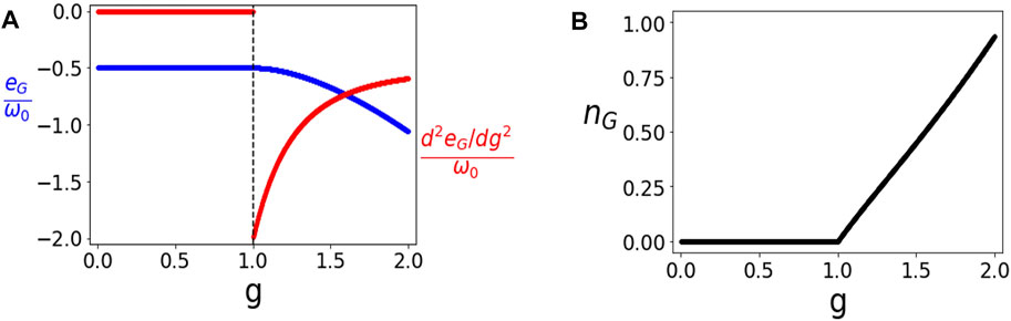
FIGURE 1. Phase Transition in Quantum Rabi Model. (A) The rescaled ground state energy $e_G/{\omega }_0=⟨H_{\mathit{Rabi}}⟩/\mathrm{\Omega }$ and (d²e_G/dg²)/ω₀ as functions of g. The discontinuity in (d²e_G/dg²)/ω₀ at g = g_c = 1 indicates a countinuous phase transition. (B) The order parameter $n_G=\frac{{\omega }_0}{\mathrm{\Omega }}⟨a^{†}a⟩$ as a function of g. n_G becomes non-zero when the Z₂ symmetry is spontaneously broken at g > g_c = 1.

We can also write effective low-energy Hamiltonians in both the normal and the superradiant phases. For g < 1, H_Rabi can be reduced to the following effective Hamiltonian [2],

$H_{np}={\omega }_0{a}^{†}a-\frac{{\omega }_0{g}^2}{4}{\left(a+a^{†}\right)}^2-\frac{\mathrm{\Omega }}{2}.(2)$

The system’s degrees of freedom have been removed by projecting to $\left|\downarrow \right.⟩\left.⟨\downarrow \right|$, since this is a low energy description. Similarly, for g > 1 the effective Hamiltonian can be written as [2],

$H_{sp}={\omega }_0{a}^{†}a-\frac{{\omega }_0}{4g^4}{\left(a+a^{†}\right)}^2-\frac{\mathrm{\Omega }}{2}\left(g^2+g^{-2}\right),(3)$

where this time around the Hamiltonian has been projected along $\left|{\downarrow }^{\pm }\right.⟩\left.⟨{\downarrow }^{\pm }\right|$. In Section 3, we’ll use H_np and H_sp to find the critical point of the model.

2.2 Finite-Size Scaling

The FSS method is widely used to determine the critical points and the critical exponents in phase transitions [1]. To demonstrate the method, consider that we have an infinite 2d system that undergoes a classical phase transition at a critical temperature T = T_c [9]. Suppose Q is a quantity that becomes singular at T = T_c with some power law behavior

$Q_{\infty }\left(T\right)\sim |T-T_c{|}^{-\omega }.(4)$

We can also think of this system as an infinite collection of infinite stripes, where the stripes are infinitely extended along one direction and stacked along the perpendicular direction. Now suppose there are only an N number of stripes. If N is finite, Q should be regular at T = T_c since finite systems cannot have non-analyticities at T ≠ 0. The singularity at T = T_c should appear only when N → ∞. The finite size scaling hypothesis assumes the existence of a scaling function F_Q such that

$Q_N\left(T\right)\simeq Q_{\infty }\left(T\right)F_Q\left(N/{\xi }_{\infty }\left(T\right)\right),(5)$

where Q_N is the observable Q for a system with N stripes and Q_∞ corresponds to the system in the thermodynamic limit. ξ_∞ is the correlation length for the infinite system. Eq. 5 is valid when N is large. The correlation length also diverges as a power law near the critical point,

${\xi }_{\infty }\left(T\right)\sim |T-T_c{|}^{-\nu }.(6)$

Substituting Eqs 4, 6 in Eq. 5,

$Q_N\left(T\right)\simeq |T-T_c{|}^{-\omega }{F}_Q\left(N|T-T_c{|}^{\nu }\right).(7)$

Since Q_N(T) should be regular at T = T_c, the scaling function should cancel the divergence due to |T − T_c|^−ω. Therefore, the scaling function should be of the form F_Q(x) ∼ x^ω/ν as x → 0. We should then have,

$Q_N\left(T_c\right)\sim N^{\omega /\nu }.(8)$

If we define a function Δ_Q(T; N, N′) such that

${\mathrm{\Delta }}_Q\left(T;N,N^{\prime }\right)=\frac{\log \left(Q_N\left(T\right)/Q_{N^{\prime }}\left(T\right)\right)}{\log \left(N/N^{\prime }\right)},(9)$

then the value of this function at T = T_c, Δ_Q(T_c; N, N′) ≃ ω/ν is independent of N and N′. Therefore, for three different values N, N′ and N′′, the curves Δ_Q(T; N, N′) and Δ_Q(T; N′, N′′) will intersect at the critical point T = T_c. This is how we can locate the critical point using the finite size scaling hypothesis.

We can also find the critical exponents ω and ν. Noting from Eq. 4 that

$\frac{\partial Q_{\infty }\left(T\right)}{\partial T}\sim |T-T_c{|}^{-\left(\omega +1\right)}.(10)$

Therefore, we should have Δ_∂Q/∂T(T_c; N, N′) ≃ (ω + 1)/ν. Define a new function Γ_ω(T; N, N′) such that

${\mathrm{\Gamma }}_{\omega }\left(T;N,N^{\prime }\right)=\frac{{\mathrm{\Delta }}_Q\left(T;N,N^{\prime }\right)}{{\mathrm{\Delta }}_{\partial Q/\partial T}\left(T;N,N^{\prime }\right)-{\mathrm{\Delta }}_Q\left(T;N,N^{\prime }\right)}.(11)$

The value of this function at the critical point Γ_ω(T_c; N, N′) ≃ ω is independent of N and N′ and gives us the critical exponent ω. Then ν can be determined using

$\nu \simeq \frac{\omega }{{\mathrm{\Delta }}_Q\left(T_c;N,N^{\prime }\right)}.(12)$

As we’ve already stated in the Introduction, this method cannot be used for the kinds of phase transitions we are interested in which occur at a finite system size. However, for such cases we can consider an extension of the approach discussed above [10–16]. In this extended approach, instead of truncating the system in the physical space, the system is truncated in the Hilbert space [16]. The FSS ansatz looks exactly the same except that N now represents the size of the set of basis states which spans the truncated Hilbert space [16]. Moreover, the temperature T will be replaced by the parameter g which is being tuned across the critical point. This approach has been shown by Kais and co-workers to work in the case of a particle in Yukawa potential [11, 13] and the calculation of electronic structure critical parameters for atomic and molecular systems [10, 12, 14–16].

2.3 Quantum Restricted Boltzmann Machine

Solving quantum many-body problems accurately has been a taxing numerical problem since the size of the wavefunction scales exponentially. The idea of taking advantage of the aspects of Machine Learning (ML) related to dimensionality reduction and feature extraction to capture the most relevant information came from the work by Carleo and Troyer [20], which introduced the idea of representing the many-body wavefunction in terms of an Artificial Neural Network (ANN) to solve for the ground states and time evolution for spin models, with a Restricted Boltzmann Machine (RBM) as the chosen architecture for this ANN. More recently, the critical behavior of the quantum Hall plateau transition based on wavefunctions has been studied in a 2D disordered electron system with the usage of a Convolutional Neural Network (CNN) [21]. However, we focus on using an RBM architecture in this work. An RBM consists of a visible layer and a hidden layer with each neuron in the visible layer connected to all neurons in the hidden layer but the neurons within a layer are not connected to each other. The quantum state is ψ expanded in the basis $\left|x\right.⟩$:

$\left|\psi \right.⟩=\sum \psi \left(x\right)\left|x\right.⟩(13)$

The Neural Network Quantum State (NQS) [20] describes the wavefunction ψ(x) to be written as ψ(x; θ), where θ represents the parameters of the RBM. ψ(x; θ) is now written in terms of the probability distribution that is obtained from the RBM as follows:

$\psi \left(x;\theta \right)\propto \sum _{\left\{h\right\}}{e}^{\frac{1}{2}\sum _i{a}_i{\sigma }_i^z+\sum _j{b}_j{h}_j+\sum _{ij}{w}_{ij}{\sigma }_i^z{h}_j}(14)$

where, ${\sigma }_i^z$ is the Pauli z operator at i^th site, ${\sigma }_i^z$ and h_j take values { + 1, − 1}, θ = {a_i, b_j, w_ij} are the trainable bias and weight parameters of the RBM. Using stochastic optimization, the energy E(θ) is minimized.

This work was extended to obtain the ground states of the Bose-Hubbard model [22] and for the application of quantum state tomography [23].

With the rapid developments in the domains of ML and Quantum Computing (QC), the appetite for integrating ideas in both of these areas has been growing considerably. The last decade has seen a surge in the application of classical ML for quantum matter, wherein these methods have been adopted to benchmark, estimate and study the properties of quantum matter [24–27], with recently showing provable classification efficiency in classifying quantum states of matter [28]. RBM based ansätzes have been shown to capture entanglement transitions [29] and using an RBM with local sparse connectivity achieves higher accuracy compared to its dense counterpart when applied to disordered quantum Ising chains [30]. The protocols and algorithms related to ML implementable on a quantum system so-called Quantum machine Learning [31] is expected to have the potential of changing the course of fundamental scientific research [32] along with industrial pursuit.

In lieu of today’s Noisy Intermediate Scale Quantum (NISQ) devices, the ideas which utilize both classical and quantum resources, such that the part of the problem which has an exponential scaling is implemented on the quantum platform while the rest are dealt with classically, are being carefully investigated for various applications. Such algorithms are known as classical-quantum hybrid algorithms. In the work by Xia and Kais [33], a modified RBM with three layers was introduced, the third layer to account for the sign of the wavefunction, to solve for the ground state energies of molecules (see Figure 2). Now, the parametrized wavefunction ψ(x; θ) is written as a function of P(x) along with a sign function s(x):

$P\left(\mathbf{x}\right)=\frac{\sum _{\left\{h\right\}}{e}^{\sum _i{a}_i{\sigma }_i^z+\sum _j{b}_j{h}_j+\sum _{ij}{w}_{ij}{\sigma }_i^z{h}_j}}{\sum _{{\mathbf{x}}^{\prime }}\sum _{\left\{h\right\}}{e}^{\sum _i{a}_i{\sigma }_i^{z^{\prime }}+\sum _j{b}_j{h}_j+\sum _{ij}{w}_{ij}{\sigma }_i^{z^{\prime }}{h}_j}}(15)$

$s\left(\mathbf{x}\right)=\tanh \left[\left(c+\sum _i{d}_i{\sigma }_i\right)\right](16)$

FIGURE 2

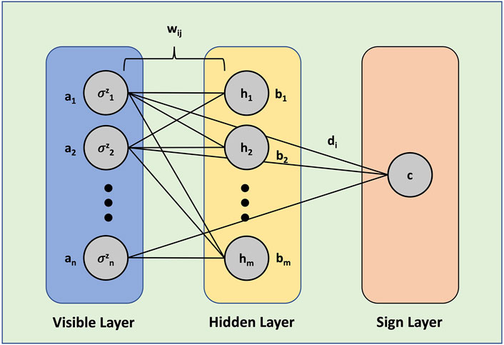
FIGURE 2. Restricted Boltzmann Machine architecture. The first layer is the visible layer with bias parameters denoted by a_i. The second layer is the hidden layer with bias parameters denoted by b_j. The third layer is the sign layer with bias parameters denoted by c. The weights associated with the connections between the visible neurons and the hidden neurons are designated by w_ij. The weights associated with the connections between the visible neurons and the neuron of the sign layer are designated by d_i.

The wavefunction ansatz in terms of the RBM can be expressed as [33]:

$\left|\psi \right.⟩=\sum _x\sqrt{P\left(x\right)}s\left(x\right)\left|x\right.⟩(17)$

A quantum circuit comprising of a single-qubit (R_y) and multi-qubit y-rotation gates (C1 − C2 − R_y) is employed, to sample the Gibbs distribution. The utilization of R_y gates caters to the bias parameter of visible and hidden layers part of the distribution, while C1 − C2 − R_y gates tend to the weights part of the distribution. In the work by Sureshbabu et al. [34], the implementation of such a circuit on IBM-Q devices was shown, wherein a new ancillary qubit is introduced to store the value corresponding to every C1 − C2 − R_y gate (Figure 3). The term n denotes the number of visible qubits and m denotes the number of hidden units. In this formalism, the number of ancillary qubits required is n × m. Starting all the qubits from a $\left|0\right.⟩$, the R_y and C1 − C2 − R_y rotations are performed, and a measurement is performed on all the qubits. If all the ancillary qubits are in $\left|1\right.⟩$, then the sampling is deemed successful and the states corresponding to the first m + n qubits provide the distribution P(x). The joint probability distribution defined over the parameters of the circuit θ = {a, b, w} and a set of y = {σ^z, h} is given by:

$P\left(y,\theta \right)=\frac{e^{\sum _i{a}_i{\sigma }_i^z+\sum _j{b}_j{h}_j+\sum _{ij}{w}_{ij}{\sigma }_i^z{h}_j}}{\sum _{\left\{y\right\}}{e}^{\sum _i{a}_i{\sigma }_i^{z^{\prime }}+\sum _j{b}_j{h}_j+\sum _{ij}{w}_{ij}{\sigma }_i^{z^{\prime }}{h}_j}}(18)$

The probability of successful sampling can be improved by rewriting the distribution P(y, θ) as Q(y, θ) and setting $k=max(1,\frac{|w_{ij}|}{2})$[33, 35]:

$Q\left(y,\theta \right)=\frac{e^{\frac{1}{k}\left(\sum _i{a}_i{\sigma }_i^z+\sum _j{b}_j{h}_j+\sum _{ij}{w}_{ij}{\sigma }_i^z{h}_j\right)}}{\sum _{\left\{y\right\}}{e}^{\frac{1}{k}\left(\sum _i{a}_i{\sigma }_i^{z^{\prime }}+\sum _j{b}_j{h}_j+\sum _{ij}{w}_{ij}{\sigma }_i^{z^{\prime }}{h}_j\right)}}(19)$

FIGURE 3

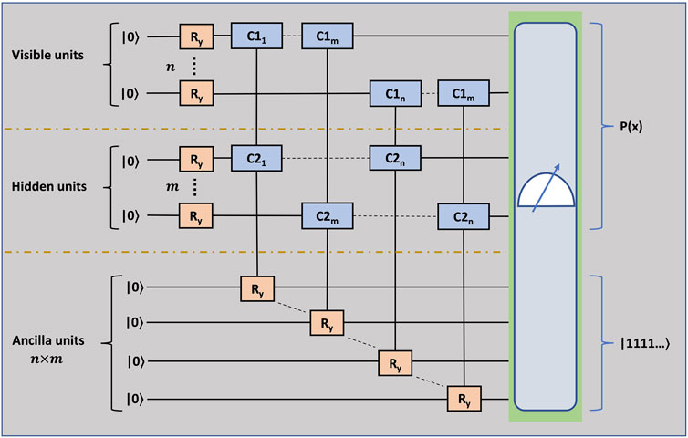
FIGURE 3. The quantum circuit to sample the Gibbs distribution. n is the number of qubits belonging to the visible layer and m is the number of qubits belonging to the hidden layer. There are m × n ancillary qubits.

Firstly, the QRBM is implemented classically, i.e., the quantum circuit is simulated on a classical computer. This execution caters to the ideal results that can be obtained through the QRBM algorithm. Then, the quantum circuit is implemented on the Digital Quantum Simulator, the qasm simulation backend. This simulator is part of the high-performance simulators from IBM-Q. The circuit is realized using IBM’s Quantum Information Software Toolkit titled Qiskit [36]. Though no noise model was utilized, as a result of finite sampling, statistical fluctuations in the values of probabilities in observing the circuit in the measurement basis, are present in the obtained results.

Having obtained the distribution Q(y, θ), the probabilities are raised to the power of k, to get P(y, θ). Following this, the sign function is computed classically, thereby calculating $\left|\psi \right.⟩$. Then, the expectation value for the Hamiltonian H $[\left.⟨\mathrm{\Psi }\right|H\left|\mathrm{\Psi }\right.⟩]$ is computed to get the energy, which is minimized using gradient descent to obtain the ground state eigenenergy of H.

The resource requirements demanded by this algorithm are quadratic. The number of qubits required are (m + n) to encode the visible and hidden nodes, and (m × n) to account for the ancillary qubits. Hence, the number of qubits scales as O(mn). The number of R_y gates required are (m + n) and the number of C1 − C2 − R_y gates required are (m × n). In addition, each C1 − C2 − R_y gate requires 6n X-gates to account for all the states spanned by the control qubits. Therefore, the number of gates required also scales as O(mn). Obtaining the ground states or minimum eigenvalues of a given matrix using exact diagonalization has a complexity of ≈ j³, with j being the dimension of the column space for the given matrix [37].

3 Results

3.1 Exact Diagonalization

In this section, we demonstrate the calculation of the critical point of the Quantum Rabi model using the Finite-Size Scaling method. As discussed before, the phase transition in QRM occurs only in the limit Ω/ω₀ → ∞. This limit is not straightforward to implement in H_Rabi given in Eq. 1. Instead, we have considered the effective low-energy Hamiltonians H_np and H_sp given in Eqs 2, 3 respectively. In H_np and H_sp, Ω is involved only in a constant term which can be removed from the Hamiltonians and the limit Ω/ω₀ → ∞ can then be easily imposed.

In H_np and H_sp, the degrees of freedom of the two-level system have been traced out and the only degrees of freedom we have are those of the bosonic mode. Let’s first consider the normal phase Hamiltonian H_np. The Hilbert space for this Hamiltonian is spanned by the familiar harmonic oscillator number states $\{\left|0\right.⟩,\left|1\right.⟩,\left|2\right.⟩,\dots \}$. We can truncate the full Hilbert space to an N-dimensional Hilbert space spanned by $\{\left|0\right.⟩,\left|1\right.⟩,\dots ,\left|N-1\right.⟩\}$ to apply the finite-size scaling analysis. In this restricted Hilbert space, the matrix form of $H_{np}^{(N)}$ can be found by using $a\left|m\right.⟩=\sqrt{m}\left|m-1\right.⟩$ and $a^{†}\left|m\right.⟩=\sqrt{m+1}\left|m+1\right.⟩$. Once we have the matrix form, we can then use the exact diagonalization method to find the ground state of $H_{np}^{(N)}$ with energy $E_{np}^{(N)}$.

Consider the scaling law for the ground state energy in the vicinity of the critical point g = g_c,

$E\left(g\right)\sim |g-g_c{|}^{\alpha }.(20)$

Here E is the ground state energy. We slightly modify the formula in Eq. 9 to take into account the difference in the signs of the exponents in Eqs 4, 20. The new formula with Q = E is,

${\mathrm{\Delta }}_{H_{np}}\left(g;N,N^{\prime }\right)=\frac{\log \left(E_{np}^{\left(N\right)}\left(g\right)/E_{np}^{\left(N^{\prime }\right)}\left(g\right)\right)}{\log \left(N^{\prime }/N\right)},(21)$

We plot the curves ${\mathrm{\Delta }}_{H_{np}}(g;N,N+2)$ for N = 8, 10, …, 30 in Figure 4A. We then plot the intersection points $g_{np}^{(N)}$ of the curves ${\mathrm{\Delta }}_{H_{np}}(g;N-4,N-2)$ and ${\mathrm{\Delta }}_{H_{np}}(g;N-2,N)$ as a function of N as shown in Figure 4B. To find the limit of $g_{np}^{(N)}$ as N → ∞, we used the Bulirsch-Stoer algorithm [44, 45]. The limit was calculated to be $g_{np}^{(N)}\to 0.999996$. So $g_c^{(np)}=0.999996$.

FIGURE 4

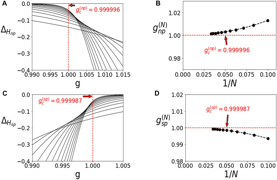
FIGURE 4. Finite-Size Scaling for Quantum Rabi model. We used N = 8, 10, …, 32. (A) Graphs of ${\mathrm{\Delta }}_{H_{np}}(g;\mathrm{8,10}),{\mathrm{\Delta }}_{H_{np}}(g;\mathrm{10,12}),\dots ,{\mathrm{\Delta }}_{H_{np}}(g;\mathrm{30,32})$ as a function of g. (B) Intersection points $g_{np}^{(N)}$ where ${\mathrm{\Delta }}_{H_{np}}(g_{np}^{(N)};N-4,N-2)={\mathrm{\Delta }}_{H_{np}}(g_{np}^{(N)};N-2,N)$, as a function of 1/N. As N → ∞, $g_{np}^{(N)}\to 0.999996$. So, $g_c^{(np)}=0.999996$. (C) Graphs of ${\mathrm{\Delta }}_{H_{sp}}(g;\mathrm{8,10}),{\mathrm{\Delta }}_{H_{sp}}(g;\mathrm{10,12}),\dots ,{\mathrm{\Delta }}_{H_{sp}}(g;\mathrm{30,32})$ as a function of g. (D) Intersection points $g_{sp}^{(N)}$ where ${\mathrm{\Delta }}_{H_{sp}}(g_{sp}^{(N)};N-4,N-2)={\mathrm{\Delta }}_{H_{sp}}(g_{sp}^{(N)};N-2,N)$, as a function of 1/N. As N → ∞, $g_{sp}^{(N)}\to 0.999987$. So, $g_c^{(sp)}=0.999987$.

In a similar way, we then consider H_sp. The curves ${\mathrm{\Delta }}_{H_{sp}}(g;N,N+2)$ are plotted in Figure 4C for N = 8, 10, …, 30 and the intersection points $g_{sp}^{(N)}$ are plotted in Figure 4D as a function of N. In this case, the extrapolation to N → ∞ gives the critical value $g_c^{(sp)}=0.999987$. Both the calculated values of $g_c^{(np)}$ and $g_c^{(sp)}$ are very close to the exact value g_c = 1.

3.2 Quantum Restricted Boltzmann Machine

Now we illustrate the implementation of the FSS method using the QRBM algorithm. The results are shown in Figure 5. Figure 5A,C show the results for H_np and H_sp using the classical implementation of the algorithm respectively. Whereas, Figure 5B,D correspond to the results for H_np and H_sp when the algorithm is implemented using the qasm simulator from IBM-Q respectively. The QRBM algorithm is run for N = 8, 10, 12, 14, 16.

FIGURE 5

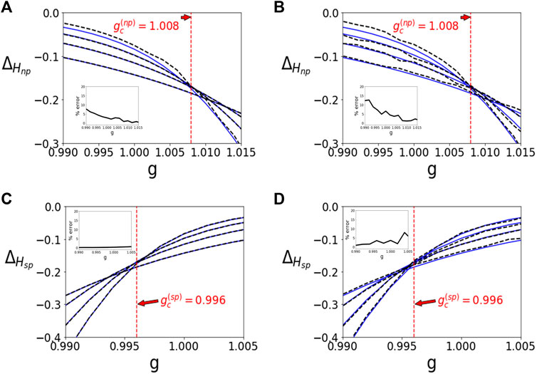
FIGURE 5. QRBM Implementation of FSS for QRM. The light blue line represents results obtained from exact diagonalization and dashed black line represents QRBM results. (A) Classical implementation of QRBM corresponding to normal phase, graphs of ${\mathrm{\Delta }}_{H_{np}}(g;\mathrm{8,10}),{\mathrm{\Delta }}_{H_{np}}(g;\mathrm{10,12}),\dots ,{\mathrm{\Delta }}_{H_{np}}(g;\mathrm{14,16})$ as a function of g. (B) QRBM implemented on qasm simulator corresponding to normal phase, graphs of ${\mathrm{\Delta }}_{H_{np}}(g;\mathrm{8,10}),{\mathrm{\Delta }}_{H_{np}}(g;\mathrm{10,12}),\dots ,{\mathrm{\Delta }}_{H_{np}}(g;\mathrm{14,16})$ as a function of g. The $g_c^{(np)}$ in both the cases is calculated to be 1.008. (C) Classical implementation of QRBM corresponding to superradiant phase, graphs of ${\mathrm{\Delta }}_{H_{sp}}(g;\mathrm{8,10}),{\mathrm{\Delta }}_{H_{sp}}(g;\mathrm{10,12}),\dots ,{\mathrm{\Delta }}_{H_{sp}}(g;\mathrm{14,16})$ as a function of g. (D) QRBM implemented on qasm simulator corresponding to superradiant phase, graphs of ${\mathrm{\Delta }}_{H_{sp}}(g;\mathrm{8,10}),{\mathrm{\Delta }}_{H_{sp}}(g;\mathrm{10,12}),\dots ,{\mathrm{\Delta }}_{H_{sp}}(g;\mathrm{14,16})$ as a function of g. The $g_c^{(sp)}$ in both the cases is calculated to be 0.996. The inset plots display the mean percentage error between the exact diagonalization results and QRBM results.

For the case of N = 8, the number of qubits associated with the visible nodes equals 3, the number of qubits associated with the hidden nodes equals 3, and 9 ancillary qubits were used. The quantum circuit consists of 6 R_y gates associated with the bias parameters, 9 C1 − C2 − R_y gates associated with the weights. Since, each C1 − C2 − R_y gate requires 6 X-gates, a total of 54 X-gates were used. For the case of N = 10,..,16, the number of qubits associated with the visible nodes equals 4, the number of qubits associated with the hidden nodes equals 4, and 16 ancillary qubits were used. The quantum circuit consists of 8 R_y gates associated with the bias parameters, 16 C1 − C2 − R_y gates associated with the weights. Since, each C1 − C2 − R_y gate requires 6 X-gates, a total of 96 X-gates were used.

Starting from random initialization, all parameters are updated via gradient descent. A learning rate of 0.01 was chosen and the algorithm is run for around 30,000 iterations. In order to assist with the convergence to the minimum eigenenergies, warm starting is employed. The method of warm starting is essentially initializing the parameters of the current point with the parameters of a previously converged point of calculation, which helps in avoiding the convergence to a local minima.

The black curves plotted in the insets in Figure 5 represent the deviation of the QRBM results (black dashed curves) from the exact diagonalization results (blue solid curves). They were calculated using the average of the quantity |Δ^(ED)(g) − Δ^(QRBM)(g)/Δ^(ED)(g)|× 100 over all the four curves. An enlarged version of the error plots is shown in Figure 6 can be found in the Supporting Information section. For each case the overall error close to g = 1.000 is not more than $\sim 5\%$ which implies convergence to the right result. Moreover, for the case of H_sp, we notice that the error is very small for the classical implementation i.e., ∼ < 1% throughout the range of the graph.

FIGURE 6

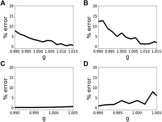
FIGURE 6. Error plots from the insets of Figure 5. (A–D) are the insets shown in Figures 5A–D respectively.

The critical point using H_np was found to be $g_c^{(np)}=1.008$ for both the classical and qasm implementations. Similarly, the critical point for the case of H_sp was found to be $g_c^{(sp)}=0.996$ for both the classical and qasm implementations. Here we notice that although, the convergence for the data obtained from both the classical and qasm implementations turns out to be the same for both H_np and H_sp, such a perfect match appears to be somewhat coincidental. Here, again the Bulirsch-Stoer algorithm [44, 45] which sets the criteria used to deduce these convergence results. The convergence plots are shown in Figure 7 have been added to the Supporting Information section.

FIGURE 7

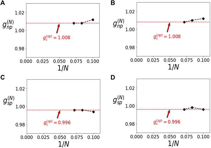
FIGURE 7. Convergence diagrams for results in Figure 5. (A–D) correspond to convergence results for data in Figures 5A–D respectively. The same procedure was used as the one shown in Figures 4B,D.

4 Discussion and Outlook

In this paper, we have used the Finite-Size Scaling in Hilbert Space approach to calculate the critical point of the Quantum Rabi Model. We used the low-energy effective Hamiltonians for both the normal and superradiant phases respectively to show that the critical point is g_c ≈ 1. The original FSS approach in which the truncation is done in the physical space has been widely used to calculate critical points and critical exponents since its inception. However, that approach was not applicable to Quantum Phase Transitions which occur at a finite system size. With the rise in interest in QPTs occurring in these finite size systems, our approach provides a natural extension of the original FSS method to study such phase transitions. To our knowledge, this is the first time this approach has been used to study a QPT in a light-matter interaction system.

We have also provided a recipe for the implementation of this method on a universal quantum computer using the Quantum Restricted Boltzmann Machine algorithm. It was shown that results obtained from the classical gate simulation match those obtained from the IBM-Q’s qasm simulator. Such an implementation scales quadratically while the exact diagonalization scales cubically in the best case and exponentially in the worst case. Looking forward, we are interested in applying this approach to other QPTs such as the QPT in anisotropic QRM. We would also like to use our method to calculate the critical exponents in addition to the critical points in these phase transitions. It would also be interesting to see if this approach can be used to predict any new phase transition for some other non-integrable model.

Another very promising research direction is to implement the FSS method for phase transitions in classically intractable many-body models such as exotic electronic and magnetic systems. These include general quantum materials, for example where Coulomb potential leads to a gapped spectrum in energy, including in direct band-gap semiconductors in the thermodynamic limit. Conventionally speaking, it might be necessary to resort to the original finite-size scaling in the physical space approach for these systems since they exhibit criticality only in the limit N → ∞. However, the ground state of an appropriately truncated Hamiltonian could be deduced using the QRBM algorithm as shown in the paper towards efficient implementation on a digital quantum simulator. A simile can also be drawn between a many-body bulk gap separating a continuum of excited states from the ground state manifold to the gapped Rabi model discussed in this paper. Such an approach can be useful in emergent topological systems, such as in Weyl semimetals, 1-D Kitaev spin chains, quantum spin liquids, and others, on which there is a tremendous explosion of interest [38–43]. Topological phase transitions are devoid of any conventional order parameter and a quantum solution deriving from the approach outlined in this paper can help us bypass resource and scaling limitations of DMRG and exact diagonalization approaches to calculate the critical point and the critical exponents.

Data Availability Statement

The original contributions presented in the study are included in the article/Supplementary Material, further inquiries can be directed to the corresponding author.

Author Contributions

SK and AB designed the research problem, BK and SS performed the calculations, all authors discussed the results and wrote the paper.

Conflict of Interest

The authors declare that the research was conducted in the absence of any commercial or financial relationships that could be construed as a potential conflict of interest.

Publisher’s Note

All claims expressed in this article are solely those of the authors and do not necessarily represent those of their affiliated organizations, or those of the publisher, the editors and the reviewers. Any product that may be evaluated in this article, or claim that may be made by its manufacturer, is not guaranteed or endorsed by the publisher.

Acknowledgments

We acknowledge funding by the US Department of Energy, Office of Science, National Quantum Information Science Research Centers, Quantum Science Center.

References

1. Goldenfeld N. Lectures on Phase Transitions and the Renormalization Group; Frontiers in Physics. Addison-Wesley Publishing Company (1992).

Google Scholar

2. Hwang M-J, Puebla R, Plenio MB. Quantum Phase Transition and Universal Dynamics in the Rabi Model. Phys Rev Lett (2015) 115:180404. doi:10.1103/physrevlett.115.180404

PubMed Abstract | CrossRef Full Text | Google Scholar

3. Hwang M-J, Plenio MB. Quantum Phase Transition in the Finite Jaynes-Cummings Lattice Systems. Phys Rev Lett (2016) 117:123602. doi:10.1103/physrevlett.117.123602

PubMed Abstract | CrossRef Full Text | Google Scholar

4. Liu M, Chesi S, Ying Z-J, Chen X, Luo H-G, Lin H-Q. Universal Scaling and Critical Exponents of the Anisotropic Quantum Rabi Model. Phys Rev Lett (2017) 119:220601. doi:10.1103/physrevlett.119.220601

PubMed Abstract | CrossRef Full Text | Google Scholar

5. Hwang M-J, Rabl P, Plenio MB. Dissipative Phase Transition in the Open Quantum Rabi Model. Phys Rev A (2018) 97:013825. doi:10.1103/physreva.97.013825

CrossRef Full Text | Google Scholar

6. Xie Y-F, Chen X-Y, Dong X-F, Chen Q-H. First-order and Continuous Quantum Phase Transitions in the Anisotropic Quantum Rabi-Stark Model. Phys Rev A (2020) 101:053803. doi:10.1103/physreva.101.053803

CrossRef Full Text | Google Scholar

7. Cai M-L, Liu Z-D, Zhao W-D, Wu Y-K, Mei Q-X, Jiang Y, et al. Observation of a Quantum Phase Transition in the Quantum Rabi Model with a Single Trapped Ion. Nat Commun (2021) 12:1126. doi:10.1038/s41467-021-21425-8

PubMed Abstract | CrossRef Full Text | Google Scholar

8. Forn-Díaz P, Lamata L, Rico E, Kono J, Solano E. Ultrastrong Coupling Regimes of Light-Matter Interaction. Rev Mod Phys (2019) 91:025005. doi:10.1103/revmodphys.91.025005

CrossRef Full Text | Google Scholar

9. Derrida B, Seze LD. In Application of the Phenomenological Renormalization to Percolation and Lattice Animals in Dimension 2. In: JL CARDY, editor. Current Physics–Sources and Comments, 2. Elsevier (1988). p. 275–83. doi:10.1016/b978-0-444-87109-1.50024-8

CrossRef Full Text | Google Scholar

10. Neirotti JP, Serra P, Kais S. Electronic Structure Critical Parameters from Finite-Size Scaling. Phys Rev Lett (1997) 79:3142–5. doi:10.1103/physrevlett.79.3142

CrossRef Full Text | Google Scholar

11. Serra P, Neirotti JP, Kais S. Finite-size Scaling Approach for the Schrödinger Equation. Phys Rev A (1998) 57:R1481–R1484. doi:10.1103/physreva.57.r1481

CrossRef Full Text | Google Scholar

12. Serra P, Neirotti JP, Kais S. Electronic Structure Critical Parameters for the Lithium Isoelectronic Series. Phys Rev Lett (1998) 80:5293–6. doi:10.1103/physrevlett.80.5293

CrossRef Full Text | Google Scholar

13. Serra P, Neirotti JP, Kais S. Finite Size Scaling in Quantum Mechanics. J Phys Chem A (1998) 102:9518–22. doi:10.1021/jp9820572

CrossRef Full Text | Google Scholar

14. Kais S, Serra P. Quantum Critical Phenomena and Stability of Atomic and Molecular Ions. Int Rev Phys Chem (2000) 19:97–121. doi:10.1080/014423500229873

CrossRef Full Text | Google Scholar

15. Shi Q, Kais S. Finite Size Scaling for Critical Parameters of Simple Diatomic Molecules. Mol Phys (2000) 98:1485–93. doi:10.1080/00268970009483354

CrossRef Full Text | Google Scholar

16. Kais S, Serra P. Finite-Size Scaling for Atomic and Molecular Systems. Adv Chem Phys (2003) 125:1–99. doi:10.1002/0471428027.ch1

CrossRef Full Text | Google Scholar

17. Francis A, Zhu D, Huerta Alderete C, Johri S, Xiao X, Freericks JK, et al. Many-body Thermodynamics on Quantum Computers via Partition Function Zeros. Sci Adv (2021) 7:eabf2447. doi:10.1126/sciadv.abf2447

PubMed Abstract | CrossRef Full Text | Google Scholar

18. Keesling A, Omran A, Levine H, Bernien H, Pichler H, Choi S, et al. Quantum Kibble–Zurek Mechanism and Critical Dynamics on a Programmable Rydberg Simulator. Nature (2019) 568:207–11. doi:10.1038/s41586-019-1070-1

PubMed Abstract | CrossRef Full Text | Google Scholar

19. Dupont M, Moore JE. Quantum Criticality Using a Superconducting Quantum Processor (2021). arXiv:2109.10909.

Google Scholar

20. Carleo G, Troyer M. Solving the Quantum many-body Problem with Artificial Neural Networks. Science (2017) 355:602–6. doi:10.1126/science.aag2302

PubMed Abstract | CrossRef Full Text | Google Scholar

21. Li Z, Luo M, Wan X. Extracting Critical Exponents by Finite-Size Scaling with Convolutional Neural Networks. Phys Rev B (2019) 99:075418. doi:10.1103/physrevb.99.075418

CrossRef Full Text | Google Scholar

22. Saito H. Solving the Bose-Hubbard Model with Machine Learning. J Phys Soc Jpn (2017) 86:093001. doi:10.7566/jpsj.86.093001

CrossRef Full Text | Google Scholar

23. Torlai G, Mazzola G, Carrasquilla J, Troyer M, Melko R, Carleo G. Neural-network Quantum State Tomography. Nat Phys (2018) 14:447–50. doi:10.1038/s41567-018-0048-5

CrossRef Full Text | Google Scholar

24. Carrasquilla J, Melko RG. Machine Learning Phases of Matter. Nat Phys (2017) 13:431–4. doi:10.1038/nphys4035

CrossRef Full Text | Google Scholar

25. Deng D-L, Li X, Das Sarma S. Machine Learning Topological States. Phys Rev B (2017) 96:195145. doi:10.1103/physrevb.96.195145

CrossRef Full Text | Google Scholar

26. Butler KT, Davies DW, Cartwright H, Isayev O, Walsh A. Machine Learning for Molecular and Materials Science. Nature (2018) 559:547–55. doi:10.1103/physrevb.96.195145

PubMed Abstract | CrossRef Full Text | Google Scholar

27. Carleo G, Cirac I, Cranmer K, Daudet L, Schuld M, Tishby N, et al. Machine Learning and the Physical Sciences. Rev Mod Phys (2019) 91:045002. doi:10.1103/revmodphys.91.045002

CrossRef Full Text | Google Scholar

28. Huang H-Y, Kueng R, Torlai G, Albert VV, Preskill J. Provably Efficient Machine Learning for Quantum many-body Problems (2021). arXiv preprint arXiv:2106.12627.

Google Scholar

29. Medina R, Vasseur R, Serbyn M. Entanglement Transitions from Restricted Boltzmann Machines. Phys Rev B (2021) 104:104205. doi:10.1103/physrevb.104.104205

CrossRef Full Text | Google Scholar

30. Pilati S, Pieri P. Simulating Disordered Quantum Ising Chains via Dense and Sparse Restricted Boltzmann Machines. Phys Rev E (2020) 101:063308. doi:10.1103/PhysRevE.101.063308

PubMed Abstract | CrossRef Full Text | Google Scholar

31. Biamonte J, Wittek P, Pancotti N, Rebentrost P, Wiebe N, Lloyd S. Quantum Machine Learning. Nature (2017) 549:195–202. doi:10.1038/nature23474

PubMed Abstract | CrossRef Full Text | Google Scholar

32. Sajjan M, Li J, Selvarajan R, Sureshbabu SH, Kale SS, Gupta R, et al. Quantum Computing Enhanced Machine Learning for Physico-Chemical Applications (2021). arXiv preprint arXiv:2111.00851.

Google Scholar

33. Xia R, Kais S. Quantum Machine Learning for Electronic Structure Calculations. Nat Commun (2018) 9:4195–6. doi:10.1038/s41467-018-06598-z

PubMed Abstract | CrossRef Full Text | Google Scholar

34. Sureshbabu SH, Sajjan M, Oh S, Kais S. Implementation of Quantum Machine Learning for Electronic Structure Calculations of Periodic Systems on Quantum Computing Devices. J Chem Inf Model (2021) 61(6):2667–2674. doi:10.1021/acs.jcim.1c00294

CrossRef Full Text | Google Scholar

35. Sajjan M, Sureshbabu SH, Kais S. Quantum Machine-Learning for Eigenstate Filtration in Two-Dimensional Materials. J Am Chem Soc (2021) 143:18426–45. doi:10.1021/jacs.1c06246

PubMed Abstract | CrossRef Full Text | Google Scholar

36. Aleksandrowicz G, Alexander T, Barkoutsos P, Bello L, Ben-Haim Y, Bucher D, et al. Qiskit: An Open-Source Framework for Quantum Computing. Zenodo (2019) 16:11. doi:10.5281/zenodo.2562111

CrossRef Full Text | Google Scholar

37. Harris CR, Millman KJ, van der Walt S, Gommers R, Virtanen P, Cournapeau D, et al. Array Programming with NumPy. Nature (2020) 585:357–62. doi:10.1038/s41586-020-2649-2

PubMed Abstract | CrossRef Full Text | Google Scholar

38. Satzinger KJ, Liu YJ, Smith A, Knapp C, Newman M, Jones C, et al. Realizing Topologically Ordered States on a Quantum Processor. Science (2021) 374:1237–41. doi:10.1126/science.abi8378

PubMed Abstract | CrossRef Full Text | Google Scholar

39. Kitaev A. Anyons in an Exactly Solved Model and beyond. Ann Phys (2006) 321:2–111. January Special Issue. doi:10.1016/j.aop.2005.10.005

CrossRef Full Text | Google Scholar

40. Liu Y-J, Shtengel K, Smith A, Pollmann F. Methods for Simulating String-Net States and Anyons on a Digital Quantum Computer. arXiv:2110.02020 2021.

Google Scholar

41. Xiao X, Freericks JK, Kemper AF. Determining Quantum Phase Diagrams of Topological Kitaev-Inspired Models on NISQ Quantum Hardware. Quantum (2021) 5:553. doi:10.22331/q-2021-09-28-553

CrossRef Full Text | Google Scholar

42. Wen X-G. Colloquium: Zoo of Quantum-Topological Phases of Matter. Rev Mod Phys (2017) 89:041004. doi:10.1103/revmodphys.89.041004

CrossRef Full Text | Google Scholar

43. Hasan MZ, Kane CL. Colloquium: Topological Insulators. Rev Mod Phys (2010) 82:3045–67. doi:10.1103/revmodphys.82.3045

CrossRef Full Text | Google Scholar

44. Bulirsch R, Stoer J. Numerical Treatment of Ordinary Differential Equations by Extrapolation Methods. Numer Math (1966) 8:1–13. doi:10.1007/bf02165234

CrossRef Full Text | Google Scholar

45. Henkel M, Schutz G. Finite-lattice Extrapolation Algorithms. J Phys A: Math Gen (1988) 21:2617–33. doi:10.1088/0305-4470/21/11/019

CrossRef Full Text | Google Scholar

Appendix A:

Bulirsch-Stoer Algorithm

For h_N = 1/N where N = 0, 1, 2, …, the Bulirsch-Stoer algorithm can be used to find the limit of a function T(h_N) as N → ∞^44,45. For demonstration, consider that we only have T(h_N) for N = 0, 1, 2, 3, then the following rows are computed successively,

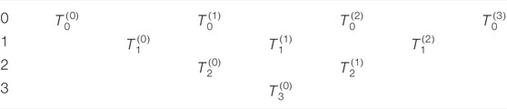
using the following rules

$T_{-1}^{\left(N\right)}=0(22)$

$T_0^{\left(N\right)}=T\left(h_N\right)(23)$

$T_{m\ge 1}^{\left(N\right)}=T_{m-1}^{\left(N+1\right)}+\left(T_{m-1}^{\left(N+1\right)}-T_{m-1}^{\left(N\right)}\right){\left[{\left(\frac{h_N}{h_{N+m}}\right)}^{\omega }\left(1-\frac{T_{m-1}^{\left(N+1\right)}-T_{m-1}^{\left(N\right)}}{T_{m-1}^{\left(N+1\right)}-T_{m-2}^{\left(N+1\right)}}\right)-1\right]}^{-1}(24)$

where ω is a free parameter determined by minimizing ${\epsilon }_m^{(i)}=|T_m^{(i+1)}-T_m^{(i)}|$. The final answer is $T_3^{(0)}$.