Boundaries control active channel flows

1 Introduction

Active fluids are composed of active entities, such as bacteria [1, 2], biofilaments driven by motor proteins [3, 4] or self-propelled colloids [5, 6], that consume energy to generate their own motion. Such active particles exert dipolar forces on their surroundings, driving self-sustained active flows. The elongated nature of the active units endows the fluid with liquid crystalline degrees of freedom, allowing for the onset of orientational order, with either polar or nematic symmetry [7].

The orientationally ordered state of bulk active fluids is generically unstable at all activities due to the feedback between deformations and flow [8], resulting in spatiotemporal chaotic dynamics at zero Reynolds number that has been referred to as bacterial or active turbulence [9]. Several strategies have been proposed to stabilize laminar flows in active fluids such as the inclusion of substrate friction [10–13] or spatial confinement [14–20], but a systematic treatment unifying these various results has remained elusive.

The dynamics of confined two-dimensional (2D) active fluids also depends on the symmetry of local order, though some features are common. Polar active fluids, such as dense suspensions of swimming bacteria, transition from laminar to undulating and periodic travelling flows upon increasing the channel width, eventually giving place to turbulent dynamics [21–24]. In active nematics, both numerical studies [25–28] and experiments with microtubule-kinesin suspensions [29] with strong anchoring to the channel walls have revealed a transition from laminar to oscillatory flows to a lattice of counter-rotating flow vortices with associated order of disclinations in the nematic texture. Similar flow states and transitions are also reported in other geometries, such as in circular confinement [15, 19, 30]. Recent work has also begun exploring the influence of varying and conflicting anchoring boundary conditions in active nematics in channels [24, 31]. In general the interplay of the geometry of confinement and boundary conditions yields a rich variety of flow states, but coherent flow with a finite throughput in the channel is only achieved by finely tuning activity and other system parameters. Hence, quantifying the conditions that yield specific flow patterns, and especially identifying states of finite throughput is important for controlling bacterial flow through channels and for microfluidic applications of active flows [32–36].

Motivated by the sensitivity of liquid crystals to surface effects and anchoring on the boundary [37], in this paper, we suggest a simple strategy to control channel flows of active fluids by tuning boundary conditions. We consider an incompressible polar active fluid confined to a two-dimensional (2D) channel with friction, and examine the role of parallel surface anchoring in selecting the spontaneously flowing states of the fluid. The model may be appropriate, for instance, to describe the spontaneous flow of a bacterial suspension in a channel. We show that the selection of the flow patterns is controlled by the interplay of two length scales: 1) the hydrodynamic screening length ${\ell }_{\eta }=\sqrt{\eta /\mathrm{\Gamma }}$ that quantifies the scale beyond which dissipation by substrate friction (Γ) dominates over dissipation from internal shear viscosity (η), and 2) the extrapolation length, ℓ_κ = K/E_a governing the length scale over which elastic torques controlled by the stiffness K of the polar fluid balance the wall anchoring energy E_a of the orientational degrees of freedom. The hydrodynamic length screens flows and controls the penetration of the boundary conditions on the flow field v into the bulk of the channel. The extrapolation length controls the relative strength between nematic elasticity and surface anchoring. Strong wall anchoring corresponds to a short ℓ_κ, while weak anchoring corresponds to large ℓ_κ [37].

We find that coherent active flows with finite throughput are only possible when the orientational order parameter is weakly anchored to the channel walls, corresponding to large ℓ_κ compared to the width W of the channel. In the opposite limit of strong anchoring, the spontaneous flow transition leads instead to a single file of flow vortices evenly spaced along the length of the channel that we refer to as flow vortex lattice. These vortices appear in counter-rotating pairs and their number is determined by the aspect ratio of the channel and the activity. The succession of flow states obtained when activity is increased above the spontaneous flow instability on the way to turbulence are summarized schematically in Figure 1 for both weak and strong homogeneous anchoring. For weak anchoring, the spontaneous flow transition leads to coherent laminar flow and associated splay deformation of the polarization field. At higher activity the system settles into a state of shear banded flow, with bend deformations of the polarization field across the channel. For strong anchoring, in contrast, the spontaneous flow instability first results in a lattice of flow vortices lined up along the channel, with longitudinal bend deformations of the polarization. At higher activity this gives way to the shear banded flow as for weak anchoring, albeit with stronger amplitude of polarization deformations. For all anchoring strengths, the flow eventually becomes chaotic at larger activity (not shown). By considering variable boundary conditions, we unify previous results in a comprehensive phase diagram that crucially combines the well-known active length scale ${\ell }_{\alpha }=\sqrt{K/|{\alpha }_0|}$ (α₀ measuring the strength of the active stress) [38, 39] controlling patterns in the bulk of the fluid along with boundary related length scales in both flow (ℓ_η) and order (ℓ_κ).

FIGURE 1

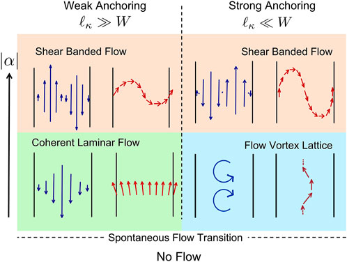
FIGURE 1. Schematic showing the effect of wall anchoring of the polarization on the steady flow states of a polar active fluid in a channel of width W. The blue arrows depict the flow field, v, and the red arrows represent the polarization, p. The extended arrow on the left indicates the direction of increasing activity |α|.

In the rest of the paper, we first introduce the hydrodynamic model and the boundary conditions used in the channel geometry. In section 3 we report results from numerical solutions of the continuum equations and describe the various spontaneous flow states observed with increasing activity. We define and evaluate the mean normalized throughput through the channel to distinguish between coherent and non-coherent flows. In section 4 we present a linear stability analysis of the hydrodynamic model for a rectangular periodic box that qualitatively accounts for the transitions between the various flow states. The results are summarized in a comprehensive phase diagram in terms of activity, hydrodynamic screening and anchoring strength. In Section 5 we discuss the effect of a polar propulsive force in the momentum equation which breaks flow symmetry and destroys the non-flowing ordered state. Finally, we conclude with a discussion of potential experimental realisations and possible extensions of our work.

2 Hydrodynamic model

We consider a two-dimensional active polar fluid on a frictional substrate, as appropriate, for instance, to describe a thin film of a bacterial suspension [40]. At high bacterial concentration, we assume both the suspension density and the bacterial concentration to be constant and describe the dynamics in terms of two fields, the bacterial polarization p that characterizes the local direction of bacterial motility and the flow velocity v of the fluid.

The dynamics of the polarization is governed by

$D_t\mathbf{p}=\lambda \mathbf{S}\cdot \mathbf{p}+\frac{1}{\gamma }\mathbf{h},(1)$

where D_tp = ∂_tp + v ⋅∇p + Ω ⋅p is the material derivative that embodies advection and rotation of polarization by flow, with $\mathbf{\Omega }=\left(\nabla \mathbf{v}-{\nabla \mathbf{v}}^T\right)/2$ the vorticity tensor. The first term on the right-hand side of Eq. 1 describes flow alignment, with $\mathbf{S}=\left(\nabla \mathbf{v}+{\nabla \mathbf{v}}^T\right)/2$ the strain rate tensor and λ a microscopic parameter that depends on the shape of the active entities (λ > 1 for elongated swimmers). The second term is the molecular field that drives relaxation with a rate set by the rotational viscosity γ. It is determined by a Landau free energy as h = −δF/δp, with

$F=\frac{1}{2}{\int }_{\mathbf{r}}\left\{K{\left({\partial }_i{p}_j\right)}^2-a\left(\frac{c}{c_0}-1\right){\mathbf{p}}^2+\frac{b}{2}{\mathbf{p}}^4\right\},(2)$

where a, b > 0 and the bacterial concentration c controls the transition to polar order. Here, we have assumed that a single elastic constant K controls the stiffness to both bend and splay distortions. For simplicity we neglect in Eq. 1 flow alignment terms proportional to v which arise through a lubrication approximation [40]. We have verified that these terms do not qualitatively change our results.

At low Reynolds number the flow is governed by force balance through the Stokes equation,

$\mathrm{\Gamma }\mathbf{v}=-\nabla \mathrm{\Pi }+\eta {\nabla }^2\mathbf{v}+\nabla \cdot \left({\mathit{\sigma }}^{\text{a}}+{\mathit{\sigma }}^{\text{lc}}\right),(3)$

where the pressure Π is determined by the condition of incompressibility, ∇ ⋅v = 0. Here, Γ is the friction with the substrate. Dissipation is controlled by the interplay of friction and viscosity η, with ${\ell }_{\eta }=\sqrt{\eta /\mathrm{\Gamma }}$ the viscous screening length that controls the penetration of the no-slip boundary conditions into the channel. The passive liquid-crystalline stress, σ^lc, describes the elastic stresses due to distortions of the polarization field and is given by

${\mathit{\sigma }}^{\text{lc}}=-\frac{\lambda +1}{2}\mathbf{p}\mathbf{h}-\frac{\lambda -1}{2}\mathbf{h}\mathbf{p}+K\nabla p_i\nabla p_i.(4)$

Finally, the dipolar forces exerted by the swimmers on the fluid yield an active stress σ^a [7],

${\mathit{\sigma }}^{\text{a}}={\alpha }_0\left(\mathbf{p}\mathbf{p}-\frac{|\mathbf{p}{|}^2}{2}\mathbf{I}\right),(5)$

where the activity α₀ provides a measure of the strength of active forces, depending, for instance, on bacterial concentration and swimming speed. Its sign depends on whether such forces are extensile (α₀ < 0 as for pushers) or contractile (α₀ > 0 as for pullers). Here we focus on extensile active forces which are relevant to most bacteria. Note that, other sources of activity such as self-advection are neglected here for simplicity, and their effects are briefly discussed later in Section 5.

We assume that the fluid is confined to a channel of width W and length L, in the geometry shown in Figure 2, with periodic boundary conditions along the y direction. Below we focus on the dynamics of the ordered state with c > c₀ and $\mathbf{p}=\sqrt{a/b}\widehat{\mathbf{y}}$. We normalize the polarization so that |p| = 1 in the aligned state.

FIGURE 2

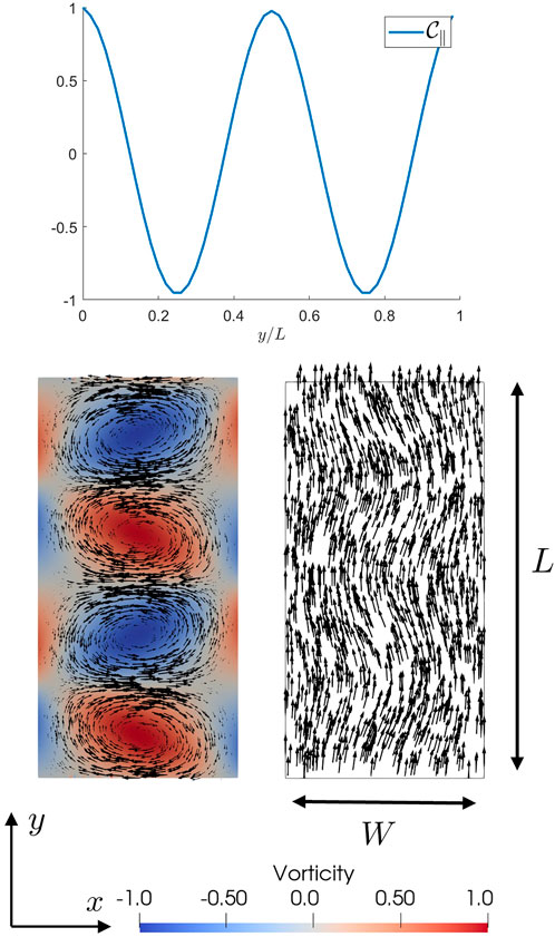
FIGURE 2. The velocity correlation function along the channel, C_∥, for the vortex lattice state (ℓ_η = 0.30, α = −2.00) with strong anchoring (ℓ_κ = 0.01). The flow profile v (bottom left) and polarization p (bottom right) in the vortex lattice state are plotted at the bottom.

The hydrodynamic equations are solved with the boundary conditions.

${\left.\mathbf{v}\right|}_{x=0,W}=0,(6)$

${\left[E_a\left(\mathbf{p}-\widehat{\mathbf{y}}\right)+K\left(\widehat{\mathbf{n}}\cdot \nabla \mathbf{p}\right)\right]}_{x=0,W}=0,(7)$

Where $\widehat{\mathbf{n}}$ is a unit normal pointing outward from the walls. The boundary condition on the polarization expresses the balance between a torque E_ap_x that penalizes misalignment with the boundary, with E_a an anchoring energy per unit length, and the nematic torque K∂_xp_x that penalizes deviations from the aligned state. The ratio ℓ_κ = K/E_a defines the extrapolation length [37], with the following limiting cases

$\begin{array}{cc}\hfill {\ell }_{\kappa }\to 0:& {\left[\mathbf{p}\right]}_{x=0,W}=\widehat{\mathbf{y}}\mathrm{s}\mathrm{t}\mathrm{r}\mathrm{o}\mathrm{n}\mathrm{g}\mathrm{a}\mathrm{n}\mathrm{c}\mathrm{h}\mathrm{o}\mathrm{r}\mathrm{i}\mathrm{n}\mathrm{g}\hfill \\ \hfill {\ell }_{\kappa }\to \infty :& {\left[{\partial }_x\mathbf{p}\right]}_{x=0,W}=\mathbf{0}\mathrm{w}\mathrm{e}\mathrm{a}\mathrm{k}\mathrm{a}\mathrm{n}\mathrm{c}\mathrm{h}\mathrm{o}\mathrm{r}\mathrm{i}\mathrm{n}\mathrm{g}\hfill \end{array}$

The hydrodynamic equations for our model have nematic symmetry, as they are invariant for p → −p. The boundary conditions, however, break the symmetry in polarization by aligning p with the channel walls in $\widehat{\mathbf{y}}$ direction. As we will discuss later in Section 5, this still allows for symmetry in the flow direction, which can by broken by introducing an active self propulsion term in Eq. 3.

3 Numerical simulations

The hydrodynamic equations are solved numerically using the finite element platform FEniCs [41, 42]. We use the width of the channel, W, as unit of length, the nematic relaxation time, τ_n = γ/a, as unit of time and the condensation energy a in the polar free energy as a unit of stress. With this choice, the dimensionless activity $\alpha =|{\alpha }_0|/a={({\ell }_{\alpha }/\xi )}^2$ is simply the square of the ratio between the active length ${\ell }_{\alpha }=\sqrt{K/|{\alpha }_0|}$ and the nematic correlation length $\xi =\sqrt{K/a}$. Unless specified otherwise, the results are shown for channel dimensions with L = 2W, flow alignment parameter λ = 2, and nematic correlation length ξ = 0.1W. To carry out the finite element simulations, the channel is triangulated into a rectangular mesh with grid size dx ∼ 0.01W. The time step used in most simulations is dt = τ_n/10 and we typically run simulations for a total time T = 1000τ_n or longer.

In bulk, an extensile active fluid ordered along y, is destabilized at any value of activity by the unbounded growth of bend fluctuations δp_x (y, t) of the order parameter [8, 14]. Both substrate friction (Γ) and a finite system size (L along the y direction) generate a finite activity threshold for the onset of spontaneous flow given by [12, 43].

${\alpha }_c^b=\frac{2K\mathrm{\Gamma }}{\gamma \left(\lambda +1\right)}\left[1+{\left(\frac{2\pi {\ell }_{\eta }}{L}\right)}^2\right].(8)$

For vanishing friction (Γ → 0), the screening length diverges (ℓ_η → ∞) and we recover the viscous limit of the finite size activity threshold ${\alpha }_c^L=(2K\eta /\gamma (\lambda +1)){(2\pi /L)}^2$ [14].

As shown below, wall anchoring geometrically frustrates this bulk instability mode and alters the mechanisms and nature of the instability which is now controlled by an interplay of three length scales: the channel width W, the flow screening length ℓ_η and the extrapolation length ℓ_κ.

Upon increasing activity, the quiescent state in a channel is destabilized, driving the system through a succession of flowing states. To classify such dynamical states, we examine the velocity correlation function parallel to the channel, defined as

$C_{\parallel }\left(y\right)={⟨\mathbf{v}\left(\mathbf{r}\right)\cdot \mathbf{v}\left(\mathbf{r}+y\widehat{\mathbf{y}}\right)⟩}_{\mathbf{r}},(9)$

where ⟨⋅⟩_r denotes a spatial average over the entire channel domain. The number of oscillations in the correlation function is used to classify the nature of the flow; see Figure 2 for an example of a flow state (the vortex lattice) with the associated correlation function plotted.

While C_∥ captures vorticity in flow patterns, states with finite throughput are quantified by evaluating the normalized throughput

$\varphi =\left|{⟨\frac{v_y}{|\mathbf{v}|}⟩}_{\mathbf{r}}\right|,(10)$

where ⟨|v|⟩_r is the mean velocity.

3.1 Strong anchoring, ℓ_κ ≪ W

The flow states obtained for strong anchoring (here ℓ_κ/W = 0.01) are summarized in the phase diagram of Figure 3B obtained by varying the activity α and the screening length ℓ_η. Upon increasing activity at fixed ℓ_η, we first observe a transition from a quiescent ordered state (grey region of Figure 3B) to a flowing state (blue region) with ⟨|v|⟩ ≠ 0. Strong anchoring suppresses pure bend fluctuations. The instability is then controlled by a growing mode that necessarily has both splay and bend components, as discussed in Section 4. This is evident from the polarization profiles displayed in Figure 4B. The resulting flow is a lattice of counter-rotating flow vortices that span the channel width, with zero net throughput. We refer to this state as a “vortex lattice”.

FIGURE 3

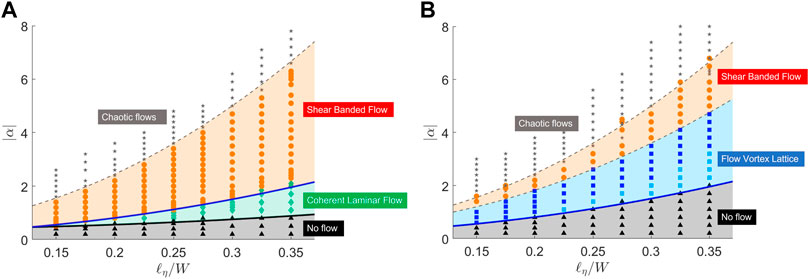
FIGURE 3. These phase diagrams show the various steady flow states in the channel as we change the screening length and the activity at a fixed anchoring strength. The dashed lines are fits to the observed phase boundaries whereas the solid lines correspond to the curves calculated using linear stability analysis in Section 4, with no fitting parameters. The solid blue line in both phase diagrams corresponds to the mixed bend-splay instability α^m and the solid black line in (B) corresponds to the splay instability with weak anchoring, α^s,w (Eq. 16). (A) Weak Anchoring, ℓ_κ/W =100. (B) Strong Anchoring, ℓ_κ/W =0.01.

FIGURE 4

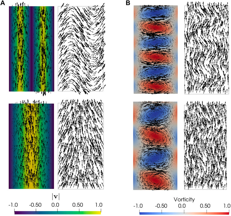
FIGURE 4. Some of the steady states observed in the phase diagrams (ℓ_η = 0.35) are shown in terms of the flow v (left in each frame) and the polarization p (right). The vorticity and the flow magnitude are colorized to show relative magnitudes and have been scaled by the corresponding maximum/minimum. The arrows represent the vectors for v and p scaled by their magnitudes. ℓ_κ. (A) Steady States with weak anchoring, ℓ_κ W =100, and low activity (bottom, α-1.75) and high activity (top, α=-4.00). (B) Steady States with strong anchoring, ℓ_κ W =0.01, and low activity (bottom, α-2.00) and high activity (top, α =-3.00).

The number n of counter-rotating vortex pairs in the vortex lattice is controlled by the aspect ratio L/W of the channel, together with the topological constraint that the net vorticity must be zero. This can be understood by comparing the energy cost of bend and splay deformations transverse and parallel to the long direction of the channel, with the number of pairs of vortices n ∼ (L/W) (A_s/A_v), where A_s and A_v are the amplitude of the polarization angle in the vortex-lattice and the shear banded flow states (Section 3.3). The minimum number of pairs of counter-rotating vortices is equal to the integer part of the aspect ratio and as we increase activity, additional vortices are added in pairs (light and dark blue points in Figure 3B).

Upon further increasing the activity, we note a transition (blue to orange in Figure 3B) from the ordered vortex lattice to a shear banded flow, with increasing number of shear bands at higher activities. This state is characterized by a bend about the short channel direction, transverse to the original orientation of the polarization field. Here, the flow and polarization are invariant along the channel. Interestingly, the flow transitions to a ‘more ordered state’ on increasing activity.

3.2 Weak anchoring, ℓ_κ ≫ W

For weak anchoring, and sufficiently large values of ℓ_η, the steady state corresponds to coherent laminar flow with finite throughput (green region in Figure 3A). But as we increase activity, an ordered vortex lattice similar to that in the strong anchoring limit forms transiently but then leads to a shear banded flow as the long time steady state (Figure 4A).

Notably, the laminar flowing state has non-zero splay but zero bend and can be seen only above a characteristic screening length ${\ell }_{\eta }^{*}$ (dependant on the extrapolation length ℓ_κ). From Figure 3A, this value ${\ell }_{\eta }^{*}\approx 0.2W$ for ℓ_κ/W = 100. This absence of coherent laminar flow at short screening length is further discussed in Section 4.

Figure 5 shows a phase diagram as a function of activity and extrapolation length, at a fixed screening ${\ell }_{\eta }=0.35>{\ell }_{\eta }^{*}$. As ℓ_κ decreases the coherent flow region for the splay state vanishes and the ordered flow vortices become stable for larger activities. We find that the transition to the flow vortex lattice (transient in the weak anchoring limit) is largely unaffected by the anchoring strength. Also, we observe that the activity threshold for the onset of unsteady chaotic flows is not affected by the extrapolation length, generalizing previous results [19, 30].

FIGURE 5

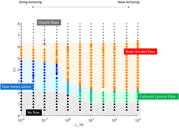
FIGURE 5. Phase diagram as we change the extrapolation length ℓ_κ at a fixed screening length ℓ_η = 0.35.

3.3 Lattice of flow vortices

Upon transition from the quiescent to the vortex state, the flow organizes into a single pair of counter-rotating vortices spanning the channel length L and of size of order L/2 (when L = 2W), as illustrated in Figure 4B for α = −2. This is observed in simulations for a large range of ℓ_η and ℓ_κ. Upon increasing activity, the number of vortex pairs increases, until eventually the system transitions to shear banded flow. The maximum number n of vortex pairs that can be accommodated in the channel depends of the channel’s aspect ratio. To estimate this number, we examine the elastic energy of channel-spanning bend deformations of the polarization field, described by the angle θ, with $\cos \theta =\mathbf{p}\cdot \widehat{\mathbf{x}}$, given by

$E\approx K{\int }_{\mathrm{\Omega }}\mathrm{d}\mathbf{r}{\left(\nabla \theta \right)}^2.(11)$

In the shear banded state, the bend deformation is primarily transverse to the channel direction (Figure 6A), corresponding to an angle profile of the form θ_s ∼ A_s sin (2πx/W). In the vortex lattice state, away from the walls, bend deformations are primarily along the length of the channel (Figure 6B), corresponding to an angle profile of the form θ_v ∼ A_v sin (2πny/L), where n is the number of counter-rotating vortex pairs. Note that the amplitudes A_s and A_v of the two deformations depend on activity and on the strength of anchoring, and are generally different.

FIGURE 6

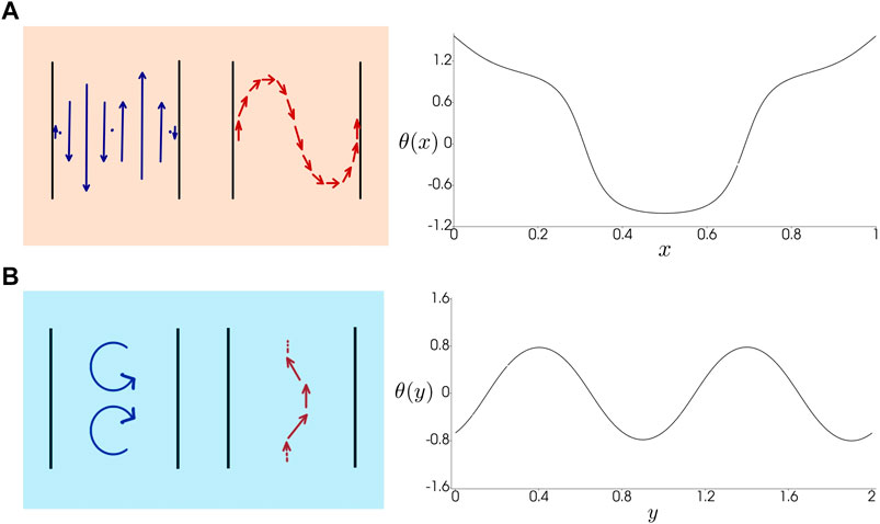
FIGURE 6. Schematic (L = W) for the shear banded and the vortex lattice flows. The line plot shows the angle θ along the polarization p for the two flow states from the numerical simulations (L = 2W) in the case of strong anchoring (ℓ_κ/W = 0.01, ℓ_η/W = 0.30). (A) Shear Banded Flow (angular profile is shown for α =-3.80). (B) Flow Vortex Lattice (angular profile is shown for α =-2.00).

The corresponding deformation energies E_s and E_v for the shear banded and flow states are then immediately obtained by substituting the respective deformations into (11), with the result $E_s=K{A}_s^{2}L/W$ and $E_v=K{n}^2{A}_v^{2}W/L$. By setting E_s ∼ E_v we can estimate the number of vortex pairs in the channel as

$n\sim \left(L/W\right)\left(A_s/A_v\right).(12)$

The scaling of the number of vortex pairs with the channel aspect ratio for the lattice of flow vortices is confirmed by numerical simulations in longer channels, as shown in Figure 7, supporting the idea that the channel geometry determines the number of flow vortices.

FIGURE 7

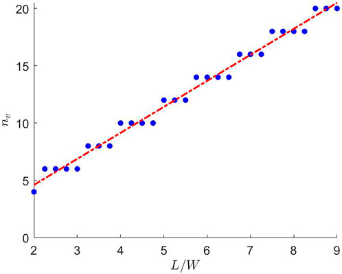
FIGURE 7. Scaling of the number of vortices, n_v, in the flow vortex lattice state for strong anchoring as a function of the channel aspect ratio L/W. The blue points correspond to n_v observed in numerical simulations (ℓ_κ = 0.01, ℓ_η = 0.35, α = −2.30) by increasing L/W in steps of 0.25 from L/W = 2 to L/W = 9. The value of n_v increases in steps of 2, corresponding to the addition of a vortex/anti-vortex pair so as to maintain zero net vorticity. The growth is linear, as predicted by the simple scaling argument given in Section 3.3, but with a slope 2.270 ± 0.005 (dashed red line).

In the limit of weak anchoring, we observe transient vortex lattices, but the stable state is always shear banded. We can understand this because in this case the system can easily accommodate bend deformations across the channel, while bend deformations along the channel, which would be required for a vortex state, are energetically more costly.

4 Linear stability analysis

The steady state channel flows summarized in the previous section can be understood using a linear stability analysis of an initial uniformly aligned state with no flow.

First, let us consider the stability of an unconfined active fluid on a frictional substrate. For small activity, the uniform quiescent state with finite polarization $\mathbf{p}=\widehat{\mathbf{y}}$ and zero flow is stable. In the absence of friction, this state is generically unstable for any activity [8, 14]. The presence of friction yields a finite activity threshold for the onset of spontaneous flow [12]. A linear stability analysis of the uniformly polarized state shows that fluctuations in the Fourier amplitude of wavevector q of the transverse component of polarization δp_x evolve as δp_x (q, t) ∼ e^ν(q)t, with the growth rate

$\nu \left(\mathbf{q}\right)=-\frac{K}{\gamma }{q}^2+\frac{|{\alpha }_0|\left(q_x^2-q_y^2\right)}{2\mathrm{\Gamma }\left(1+{\ell }_{\eta }^2{q}^2\right)}\left[\lambda \left({\widehat{q}}_x^2-{\widehat{q}}_y^2\right)-1\right]+\mathcal{O}\left(q^4\right),(13)$

where, q = |q|, ${\widehat{q}}_{x,y}=q_{x,y}/q$ and ${\ell }_{\eta }=\sqrt{\eta /\mathrm{\Gamma }}$ is the viscous screening length.

4.1 Bulk

For extensile systems (α₀ < 0) of elongated active units (λ > 1), the decay rate given in Eq. 13 can become positive, signalling the instability of the uniformly polarized state. It is known that in a bulk system, defined as one with periodic boundary conditions in all directions, the most unstable modes are bend deformations of the polarization field, corresponding to spatial variations along the direction of order, i.e., q_x = 0 and finite q_y. The hydrodynamic instability sets in at the longest wavelength, which in a periodic box of size L is 2π/L, yielding an activity threshold ${\alpha }_c^b$ (Eq. 8). Note, here the threshold is defined by its absolute value. The bend modes of wavelength 2π/L become unstable as ${\alpha }_0<-{\alpha }_c^b$ or $|{\alpha }_0|>{\alpha }_c^b$.

Viscous dissipation enters through the screening length ℓ_η and shifts the instability to higher values of activity whenever ℓ_η ∼ L. In other words, viscous dissipation stabilizes the uniform quiescent state. When ℓ_η ≪ L one recovers the infinite system frictional threshold, ${\alpha }_c^{\infty }=2K\mathrm{\Gamma }/[\gamma (\lambda +1)]$. The bulk result given in Eq. 8 fits very well with finite element simulations in a periodic box (not shown).

Upon further increasing activity, splay modes, corresponding to q_y = 0, also become unstable. This splay instability occurs above a threshold

${\alpha }_c^s=\frac{2K\mathrm{\Gamma }}{\gamma \left(\lambda -1\right)}\left[1+{\left(\frac{2\pi {\ell }_{\eta }}{W}\right)}^2\right].(14)$

Note the dependence on the width W of the channel rather than the length L. In a periodic square box (L = W), for elongated flow-aligning swimmers (λ > 1), ${\alpha }_c^s>{\alpha }_c^b$, i.e., the bend instability always precedes the splay instability in an extensile system [7]. The situation can, however, be reversed for large values of ℓ_η and suitable aspect ratios (W/L).

The angular dependence of the instability threshold is displayed in the polar plots of Figure 8, where the shaded region corresponds to unstable modes (ν(q) > 0) in the q_x − q_y plane. It is evident that the fastest growing modes are always along the q_x = 0 direction and become unstable for $|{\alpha }_0|>{\alpha }_c^b$. Pure splay modes (corresponding to q_y = 0) are stable for $|{\alpha }_0|<{\alpha }_c^s$ (Figure 8A) and only become unstable for $|{\alpha }_0|>{\alpha }_c^s$, as evident by the emergence of the two additional lobes elongated along the q_x axis (Figure 8B).

FIGURE 8

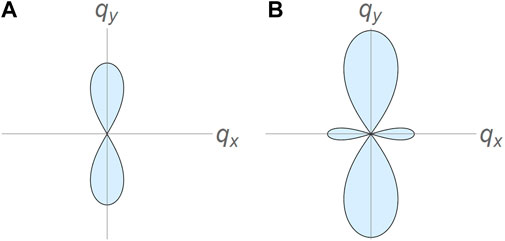
FIGURE 8. The shaded region in the q_x-q_y plane corresponds to unstable modes (ν > 0) in an extensile active fluid. Beyond the critical activity ${\alpha }_c^b$ only the bend modes (q_x = 0) become unstable. Further increasing the activity beyond ${\alpha }_c^s$, pure splay modes (q_y = 0) also become unstable. (A) ${\alpha }_b^c$ < α₀ < ${\alpha }_c^s$. (B) α₀ > ${\alpha }_c^s$.

4.2 Channel

In a channel geometry, boundary conditions can differentially frustrate bend and splay distortions [31, 44], allowing for distinct modes of spontaneous flow transitions to emerge. As in Ref. [12], we first consider a quasi-1D model that assumes only spatial variations along the direction x of the channel width. This is consistent with the observation that in the channel bend fluctuations (q_y ≠ 0) are suppressed either by strong anchoring requiring p_x = 0 at the boundaries [12, 14] and/or by the condition of no-slip. The instability to spontaneous flow is then controlled by splay fluctuations (q_x ≠ 0) and the threshold activity generally depends on the anchoring length, ℓ_κ. For strong anchoring (ℓ_κ → 0) the no-slip requirement on the velocity further excludes the possibility of a mode with wavelength 2W. Hence the longest allowed wavelength corresponds to q_x = 2π/W and the splay (s) instability threshold for the case of strong anchoring 1) can be estimated as

${\alpha }_c^{s,a}=\frac{2K\mathrm{\Gamma }}{\gamma \left(\lambda -1\right)}\left[1+{\left(\frac{2\pi {\ell }_{\eta }}{W}\right)}^2\right],{\ell }_{\kappa }=0.(15)$

For weak anchoring (ℓ_κ → ∞) conversely ∂_xp_x = 0 at the boundaries, allowing for a cosine wave of wavelength 2W instead that also satisfies no-slip. Hence the splay (s) instability threshold for the case of weak anchoring (w) is estimated as

${\alpha }_c^{s,w}=\frac{2K\mathrm{\Gamma }}{\gamma \left(\lambda -1\right)}\left[1+{\left(\frac{\pi {\ell }_{\eta }}{W}\right)}^2\right];{\ell }_{\kappa }\to \infty (16)$

In the case of weak anchoring, this simple argument provides a good estimate for the transition from the quiescent state to the coherent laminar flow. This is shown in Figure 3A by comparing the expression for ${\alpha }_c^{s,w}$ (Eq. 16, shown as a solid black line) to the spontaneous flow transition observed in numerical simulations. On the other hand, this one dimensional model fails to account for the onset of the vortex lattice with strong anchoring.

The transition to the vortex lattice can be described as arising from the instability of a mixed bend-splay mode where both q_x, q_y ≠ 0. To capture this instability, we fix the transverse wave number as $q_x=q_x^{*}$ and then determine the critical activity above which the eigenvalue $\nu (q_x=q_x^{*},q_y)$ becomes positive. Figure 5 indicates that the transition to the vortex lattice state depends only weakly on the strength of anchoring. For this reason we simply take $q_x^{*}=\pi /W$, as suggested by the fact that vortices typically have the size of the channel width at onset. The resulting critical activity for the transition to the vortex lattice state (which we refer to as a mixed instability and denote by ${\alpha }_c^m$) is compared in Figure 9 to the splay lines given by Eqs 15, 16 for the case of strong and weak anchoring, respectively. The critical activity ${\alpha }_c^m$ is computed numerically by using the dispersion relation (Eq. 13), and computing the smallest activity such that we have an unstable mode with q_x = π/W. For weak anchoring (Figure 3A), the splay instability line α^s,w (solid black line) falls below the mixed instability ${\alpha }_c^m$ (solid blue line) signaling the onset of banded flow, allowing for an intervening region of coherent laminar flow shown in green. For strong anchoring (Figure 3B), the splay instability line α_s,w is always above the mixed instability line ${\alpha }_c^m$ (solid blue line). The splay line is therefore not shown in the figure and the systems transitions directly from the quiescent state to the vortex lattice.

FIGURE 9

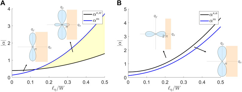
FIGURE 9. Linear instability for splay and the vortex-lattice state in the limits of weak and strong anchoring. In the insets, the orange regions delineate the values of wavector where the instability can occur, as discussed in Section 4.2. The yellow shaded region marks the range of parameters where ${\alpha }_c^{s,w}<{\alpha }_c^m$, allowing for a region of coherent flow. For the strong anchoring limit, ${\alpha }_c^m$ is always smaller than ${\alpha }_c^{s,a}$ and no coherent flow is possible. (A) Weak Anchoring (${\ell }_{\kappa }\to \infty$). (B) Strong Anchoring (${\ell }_{\kappa }$ =0).

5 Role of self propulsion

Throughout the discussion we have described the bacterial fluid using a polar order parameter, p but the model considered has nematic symmetry. In this case the flow arises from spontaneous symmetry breaking of the quiescent state and is entirely determined by deformations of the polarization field. The direction of flow is equally likely to be up or down the channel, with associated “splay-in” and “splay-out” configurations of polarization. In the simulations with finite anchoring this symmetry is broken externally by the boundary conditions on the polarization. The presence of a frictional substrate can, however, allow an additional propulsive force linear in p to be present in force balance [40, 45, 46] which takes the form

$\mathrm{\Gamma }\left(\mathbf{v}-v_0\mathbf{p}\right)=-\nabla \mathrm{\Pi }+\eta {\nabla }^2\mathbf{v}+\nabla \cdot \left({\mathit{\sigma }}^{\text{a}}+{\mathit{\sigma }}^{\text{lc}}\right).(17)$

This polar active force explicitly breaks the up-down symmetry of the flow. The homogeneous state in bulk is now a uniformly flowing state with v = v₀p. As a result, any finite self-propulsion v₀ then breaks the flow symmetry and selects the direction of the flowing state. A small self-propulsion provides therefore the minimal forcing required for creating sustained unidirectional channel flows. For small values of v₀, corresponding to v₀ ≪|α₀|/Γℓ_η, the dipolar active stress dominates over the propulsive force and the structure of the steady state flows is qualitatively unaffected. Above the critical activity for spontaneous flow, we recover coherent laminar flows arising from polarization splay for weak anchoring and flow vortex lattices for strong anchoring, as in the absence of polar self propulsion. The flow lattice, however, acquires a steady drift at speed proportional to v₀.

6 Discussion

Using a hydrodynamic model of extensile polar active matter, we have examined the role of confinement and boundary alignment in controlling the spatial and temporal organizations of active flows in a channel. We show that surface anchoring controls the flow structures by selectively frustrating bend or splay distortions in the polarization and that flows with finite throughput can only be obtained with weak surface anchoring. Strong surface anchoring leads to the formation of lattices of flow vortices, with the number of vortices determined by the aspect ratio of the channel, consistent with previous results [25, 26].

Our hydrodynamic model is inherently polar as the anchoring boundary conditions (Eq. 7) imposed at the channel walls break nematic symmetry even in the absence of any polar self propulsion (Section 5). As is evident, the symmetry of the boundary conditions plays a profound role on the selection of flow states. Strong polar anchoring, where the polarization is forced to point in the same direction on both sides of the channel, prevent splay deformation and facilitate bend along the channel walls, resulting in a state of flow vortices (Figure 10, left panel). Strong antipolar anchoring, where the polarization is forced to point in opposite directions on the two sides of the channel, allows bend deformation across the channel, resulting in finite-throughput laminar flow (Figure 10, right panel). We have also examined the case of nematic anchoring where the polarization is forced to orient with the channel wall, but with no preferred direction. This was enforced by requiring

${\left[\left(\mathbf{p}\cdot \widehat{\mathbf{n}}\right)\widehat{\mathbf{n}}+{\ell }_{\kappa }\left(\widehat{\mathbf{n}}\cdot \nabla \mathbf{p}\right)\right]}_{x=0,W}=0.(18)$

FIGURE 10

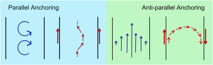
FIGURE 10. The symmetry of the boundary conditions for the polarization controls the steady flow states. Left frame: strong polar anchoring where the polarization is anchored in the same direction on both channel walls suppresses splay deformations and yields bend deformation along the wall with associated flow vortices. Right frame: strong apolar anchoring where the polarization is anchored in opposite directions on the two walls explicitly breaks the nematic symmetry even in the absence of polar self propulsion (v₀ = 0) and leads to coherent flow. Both flow states can occur if the boundary conditions are nematic, i.e., agnostic to the direction of the polarization vector.

In this case both flow states depicted in Figure 10 coexist in the phase diagram. Finally, we note that the lattice of flow vortices reported here is distinct from the state of dancing half-integer disclinations found earlier in active nematics confined to channels [47]. Here we consider a polar system, where defect in the polarization texture are +1 and −1 vortices. Such defects are indeed observed in the turbulent state at high activity. The lattice of flow vortices reported here is, however, a defect-free steady state.

Our work quantifies the role surface anchoring in controlling the spatio-temporal structure of confined active flows. This understanding can be useful for the design of active microfluidic devices where channel dimensions and boundary preparation can be independently tuned to control viscous screening and anchoring, respectively.

Recent experiments on microtubule suspensions in 3D and associated numerical studies have demonstrated that coherent flow is only possible for finely tuned geometries [17, 48–50]. Our work suggests that it would be interesting to additionally explore the role of anchoring in these 3D systems where antagonistic boundary conditions on the three walls could result in as of yet unexplored states.

Finally, it would also be interesting to explore the role of surface anchoring on temporal as well as spatial organization of active flows. Recent experiments in dense bacterial suspensions [51] have revealed that viscoelasticity of the suspending medium can drive a circular droplet to self-organize in time-periodic states of vortical flow, consisting of a system-spanning vortex that switches its chirality at a rate controlled by the solvent relaxation time. The vortex state of a circular drops corresponds to unidirectional laminar flow in a channel. As we have seen, the direction of the flow is directly determined by the splay-in or splay-out configuration of the polarization field, which in turn can be controlled with suitable anchoring. This suggest that anchoring may play an important role in controlling temporal as well as spatial organization and that it may be possible to control oscillations between flows of opposite chirality by tuning the boundary conditions. These questions are left for future studies.

Data availability statement

The raw data supporting the conclusion of this article will be made available by the authors, without undue reservation.

Author contributions

PG performed the numerical simulations and prepared the figures. All authors contributed to the formulation of the project, the analysis of the model and the writing of the paper.

Funding

This work was directly supported by NSF grant DMR-2041459. SS acknowledges support from the Harvard Society of Fellows. Use was made of computational facilities purchased with funds from the National Science Foundation (CNS-1725797) and administered by the Center for Scientific Computing (CSC). The CSC is supported by the California NanoSystems Institute and the Materials Research Science and Engineering Center (MRSEC; NSF DMR 1720256) at UC Santa Barbara.

Conflict of interest

The authors declare that the research was conducted in the absence of any commercial or financial relationships that could be construed as a potential conflict of interest.

Publisher’s note

All claims expressed in this article are solely those of the authors and do not necessarily represent those of their affiliated organizations, or those of the publisher, the editors and the reviewers. Any product that may be evaluated in this article, or claim that may be made by its manufacturer, is not guaranteed or endorsed by the publisher.

References

1. Wensink HH, Dunkel J, Heidenreich S, Drescher K, Goldstein RE, Löwen H, et al. Meso-scale turbulence in living fluids. Proc Natl Acad Sci U S A (2012) 109:14308–13. doi:10.1073/pnas.1202032109

PubMed Abstract | CrossRef Full Text | Google Scholar

2. Zhou S, Sokolov A, Lavrentovich OD, Aranson IS. Living liquid crystals. Proc Natl Acad Sci U S A (2014) 111:1265–70. doi:10.1073/pnas.1321926111

PubMed Abstract | CrossRef Full Text | Google Scholar

3. Sanchez T, Chen DT, DeCamp SJ, Heymann M, Dogic Z. Spontaneous motion in hierarchically assembled active matter. Nature (2012) 491:431–4. doi:10.1038/nature11591

PubMed Abstract | CrossRef Full Text | Google Scholar

4. Schaller V, Weber C, Semmrich C, Frey E, Bausch AR. Polar patterns of driven filaments. Nature (2010) 467:73–7. doi:10.1038/nature09312

PubMed Abstract | CrossRef Full Text | Google Scholar

5. Palacci J, Sacanna S, Steinberg AP, Pine DJ, Chaikin PM. Living crystals of light-activated colloidal surfers. Science (2013) 339:936–40. doi:10.1126/science.1230020

PubMed Abstract | CrossRef Full Text | Google Scholar

6. Bricard A, Caussin JB, Desreumaux N, Dauchot O, Bartolo D. Emergence of macroscopic directed motion in populations of motile colloids. Nature (2013) 503:95–8. doi:10.1038/nature12673

PubMed Abstract | CrossRef Full Text | Google Scholar

7. Marchetti MC, Joanny JF, Ramaswamy S, Liverpool TB, Prost J, Rao M, et al. Hydrodynamics of soft active matter. Rev Mod Phys (2013) 85:1143–89. doi:10.1103/revmodphys.85.1143

CrossRef Full Text | Google Scholar

8. Simha RA, Ramaswamy S. Hydrodynamic fluctuations and instabilities in ordered suspensions of self-propelled particles. Phys Rev Lett (2002) 89:058101. doi:10.1103/physrevlett.89.058101

PubMed Abstract | CrossRef Full Text | Google Scholar

9. Alert R, Casademunt J, Joanny JF. Active turbulence. Annu Rev Condens Matter Phys (2021) 13:143–70. doi:10.1146/annurev-conmatphys-082321-035957

CrossRef Full Text | Google Scholar

10. Duclos G, Garcia S, Yevick H, Silberzan P. Perfect nematic order in confined monolayers of spindle-shaped cells. Soft matter (2014) 10:2346–53. doi:10.1039/c3sm52323c

PubMed Abstract | CrossRef Full Text | Google Scholar

11. Doostmohammadi A, Adamer MF, Thampi SP, Yeomans JM. Stabilization of active matter by flow-vortex lattices and defect ordering. Nat Commun (2016) 7:10557. doi:10.1038/ncomms10557

PubMed Abstract | CrossRef Full Text | Google Scholar

12. Duclos G, Blanch-Mercader C, Yashunsky V, Salbreux G, Joanny JF, Prost J, et al. Spontaneous shear flow in confined cellular nematics. Nat Phys (2018) 14:728–32. doi:10.1038/s41567-018-0099-7

PubMed Abstract | CrossRef Full Text | Google Scholar

13. Thijssen K, Khaladj DA, Aghvami SA, Gharbi MA, Fraden S, Yeomans JM, et al. Submersed micropatterned structures control active nematic flow, topology, and concentration. Proc Natl Acad Sci U S A (2021) 118:e2106038118. doi:10.1073/pnas.2106038118

PubMed Abstract | CrossRef Full Text | Google Scholar

14. Voituriez R, Joanny JF, Prost J. Spontaneous flow transition in active polar gels. Europhys Lett (2005) 70:404–10. doi:10.1209/epl/i2004-10501-2

CrossRef Full Text | Google Scholar

15. Wioland H, Woodhouse FG, Dunkel J, Kessler JO, Goldstein RE. Confinement stabilizes a bacterial suspension into a spiral vortex. Phys Rev Lett (2013) 110:268102. doi:10.1103/physrevlett.110.268102

PubMed Abstract | CrossRef Full Text | Google Scholar

16. Lushi E, Wioland H, Goldstein RE. Fluid flows created by swimming bacteria drive self-organization in confined suspensions. Proc Natl Acad Sci U S A (2014) 111:9733–8. doi:10.1073/pnas.1405698111

PubMed Abstract | CrossRef Full Text | Google Scholar

17. Wu KT, Hishamunda JB, Chen DT, DeCamp SJ, Chang YW, Fernández-Nieves A, et al. Transition from turbulent to coherent flows in confined three-dimensional active fluids. Science (2017) 355:eaal1979. doi:10.1126/science.aal1979

PubMed Abstract | CrossRef Full Text | Google Scholar

18. Chen S, Gao P, Gao T. Dynamics and structure of an apolar active suspension in an annulus. J Fluid Mech (2018) 835:393–405. doi:10.1017/jfm.2017.759

CrossRef Full Text | Google Scholar

19. Opathalage A, Norton MM, Juniper MP, Langeslay B, Aghvami SA, Fraden S, et al. Self-organized dynamics and the transition to turbulence of confined active nematics. Proc Natl Acad Sci U S A (2019) 116:4788–97. doi:10.1073/pnas.1816733116

PubMed Abstract | CrossRef Full Text | Google Scholar

20. You Z, Pearce DJ, Giomi L. Confinement-induced self-organization in growing bacterial colonies. Sci Adv (2021) 7:eabc8685. doi:10.1126/sciadv.abc8685

PubMed Abstract | CrossRef Full Text | Google Scholar

21. Wioland H, Lushi E, Goldstein RE. Directed collective motion of bacteria under channel confinement. New J Phys (2016) 18:075002. doi:10.1088/1367-2630/18/7/075002

CrossRef Full Text | Google Scholar

22. Tjhung E, Cates ME, Marenduzzo D. Nonequilibrium steady states in polar active fluids. Soft Matter (2011) 7:7453. doi:10.1039/c1sm05396e

CrossRef Full Text | Google Scholar

23. Giomi L, Marchetti MC, Liverpool TB. Complex spontaneous flows and concentration banding in active polar films. Phys Rev Lett (2008) 101:198101. doi:10.1103/physrevlett.101.198101

PubMed Abstract | CrossRef Full Text | Google Scholar

24. Yang X, Wang Q. Role of the active viscosity and self-propelling speed in channel flows of active polar liquid crystals. Soft Matter (2016) 12:1262–78. doi:10.1039/c5sm02115d

PubMed Abstract | CrossRef Full Text | Google Scholar

25. Chandragiri S, Doostmohammadi A, Yeomans JM, Thampi SP. Active transport in a channel: Stabilisation by flow or thermodynamics. Soft matter (2019) 15:1597–604. doi:10.1039/c8sm02103a

PubMed Abstract | CrossRef Full Text | Google Scholar

26. Shendruk TN, Doostmohammadi A, Thijssen K, Yeomans JM. Dancing disclinations in confined active nematics. Soft Matter (2017) 13:3853–62. doi:10.1039/c6sm02310j

PubMed Abstract | CrossRef Full Text | Google Scholar

27. Samui A, Yeomans JM, Thampi SP. Flow transitions and length scales of a channel-confined active nematic. Soft Matter (2021) 17:10640–8. doi:10.1039/d1sm01434j

PubMed Abstract | CrossRef Full Text | Google Scholar

28. Wagner CG, Norton MM, Park JS, Grover P. Exact coherent structures and phase space geometry of preturbulent 2d active nematic channel flow. Phys Rev Lett (2022) 128:028003. doi:10.1103/physrevlett.128.028003

PubMed Abstract | CrossRef Full Text | Google Scholar

29. Hardoüin J, Hughes R, Doostmohammadi A, Laurent J, Lopez-Leon T, Yeomans JM, et al. Reconfigurable flows and defect landscape of confined active nematics. Commun Phys (2019) 2:121. doi:10.1038/s42005-019-0221-x

CrossRef Full Text | Google Scholar

30. Norton MM, Baskaran A, Opathalage A, Langeslay B, Fraden S, Baskaran A, et al. Insensitivity of active nematic liquid crystal dynamics to topological constraints. Phys Rev E (2018) 97:012702. doi:10.1103/physreve.97.012702

PubMed Abstract | CrossRef Full Text | Google Scholar

31. Rorai C, Toschi F, Pagonabarraga I. Active nematic flows confined in a two-dimensional channel with hybrid alignment at the walls: A unified picture. Phys Rev Fluids (2021) 6:113302. doi:10.1103/physrevfluids.6.113302

CrossRef Full Text | Google Scholar

32. Poujade M, Grasland-Mongrain E, Hertzog A, Jouanneau J, Chavrier P, Ladoux B, et al. Collective migration of an epithelial monolayer in response to a model wound. Proc Natl Acad Sci U S A (2007) 104:15988–93. doi:10.1073/pnas.0705062104

PubMed Abstract | CrossRef Full Text | Google Scholar

33. Conrad JC, Poling-Skutvik R. Confined flow: Consequences and implications for bacteria and biofilms. Annu Rev Chem Biomol Eng (2018) 9:175–200. doi:10.1146/annurev-chembioeng-060817-084006

PubMed Abstract | CrossRef Full Text | Google Scholar

34. Beebe DJ, Mensing GA, Walker GM. Physics and applications of microfluidics in biology. Annu Rev Biomed Eng (2002) 4:261–86. doi:10.1146/annurev.bioeng.4.112601.125916

PubMed Abstract | CrossRef Full Text | Google Scholar

35. Clark AG, Vignjevic DM. Modes of cancer cell invasion and the role of the microenvironment. Curr Opin Cel Biol (2015) 36:13–22. doi:10.1016/j.ceb.2015.06.004

PubMed Abstract | CrossRef Full Text | Google Scholar

36. Needleman D, Dogic Z. Active matter at the interface between materials science and cell biology. Nat Rev Mater (2017) 2:17048. doi:10.1038/natrevmats.2017.48

CrossRef Full Text | Google Scholar

37. DeGennes P, Prost J. Physics of liquid crystals. Oxford: Clarendon (1994).

Google Scholar

38. Giomi L. Geometry and topology of turbulence in active nematics. Phys Rev X (2015) 5:031003. doi:10.1103/physrevx.5.031003

CrossRef Full Text | Google Scholar

39. Hemingway EJ, Mishra P, Marchetti MC, Fielding SM. Correlation lengths in hydrodynamic models of active nematics. Soft Matter (2016) 12:7943–52. doi:10.1039/c6sm00812g

PubMed Abstract | CrossRef Full Text | Google Scholar

40. Maitra A, Srivastava P, Marchetti MC, Ramaswamy S, Lenz M. Swimmer suspensions on substrates: Anomalous stability and long-range order. Phys Rev Lett (2020) 124:028002. doi:10.1103/physrevlett.124.028002

PubMed Abstract | CrossRef Full Text | Google Scholar

41. Alnæs M, Blechta J, Hake J, Johansson A, Kehlet B, Logg A, et al. The fenics project version 1.5. Archive Numer Softw (2015) 3.

Google Scholar

42. Logg A, Mardal KA, Wells G. Automated solution of differential equations by the finite element method: The FEniCS book, vol. 84. Berlin, Germany: Springer Science & Business Media (2012).

Google Scholar

43. Thampi SP, Golestanian R, Yeomans JM. Active nematic materials with substrate friction. Phys Rev E (2014) 90:062307. doi:10.1103/physreve.90.062307

PubMed Abstract | CrossRef Full Text | Google Scholar

44. Green R, Toner J, Vitelli V. Geometry of thresholdless active flow in nematic microfluidics. Phys Rev Fluids (2017) 2:104201. doi:10.1103/physrevfluids.2.104201

CrossRef Full Text | Google Scholar

45. Brotto T, Caussin JB, Lauga E, Bartolo D. Hydrodynamics of confined active fluids. Phys Rev Lett (2013) 110:038101. doi:10.1103/physrevlett.110.038101

PubMed Abstract | CrossRef Full Text | Google Scholar

46. Kumar N, Soni H, Ramaswamy S, Sood A. Flocking at a distance in active granular matter. Nat Commun (2014) 5:4688. doi:10.1038/ncomms5688

PubMed Abstract | CrossRef Full Text | Google Scholar

47. Alert R, Joanny JF, Casademunt J. Universal scaling of active nematic turbulence. Nat Phys (2020) 16:682–8. doi:10.1038/s41567-020-0854-4

CrossRef Full Text | Google Scholar

48. Chandragiri S, Doostmohammadi A, Yeomans JM, Thampi SP. Flow states and transitions of an active nematic in a three-dimensional channel. Phys Rev Lett (2020) 125:148002. doi:10.1103/physrevlett.125.148002

PubMed Abstract | CrossRef Full Text | Google Scholar

49. Chandrakar P, Varghese M, Aghvami SA, Baskaran A, Dogic Z, Duclos G, et al. Confinement controls the bend instability of three-dimensional active liquid crystals. Phys Rev Lett (2020) 125:257801. doi:10.1103/physrevlett.125.257801

PubMed Abstract | CrossRef Full Text | Google Scholar

50. Varghese M, Baskaran A, Hagan MF, Baskaran A. Confinement-induced self-pumping in 3d active fluids. Phys Rev Lett (2020) 125:268003. doi:10.1103/physrevlett.125.268003

PubMed Abstract | CrossRef Full Text | Google Scholar

51. Liu S, Shankar S, Marchetti MC, Wu Y. Viscoelastic control of spatiotemporal order in bacterial active matter. Nature (2021) 590:80–4. doi:10.1038/s41586-020-03168-6

PubMed Abstract | CrossRef Full Text | Google Scholar