A method for identifying the important node in multi-layer logistic networks

Introduction

With the development of transportation infrastructure, traffic congestion is ubiquitous around the world, which can cause huge economic losses and even increasing the accidents [1–3]. Therefore, it is of great significance to enhance the performance of logistic networks. It is found that, to destroy a complex system, only need to attack a few key nodes [4, 5]. So, it is meaningful to identify the important nodes in the logistic network and reduce the impact of traffic congestion.

Network science provides an efficient way for understanding complex networks [6–12], so it also provides good methods to identify important nodes in complex networks [13–25]. In the early years, the identification methods are generally from single structure characteristic, such as the degree centrality, betweenness centrality, closeness centrality and so on [13–15]. In recent years, scholars have tried to compare traditional methods and combine several structural characteristics to improve the identification accuracy. Lordan et al. [16] proposed a new strategy based on the Bonacich power centrality to detect the critical nodes in the air transport network. Yang et al. [17] proposed a new weighted composite index based on weighted degree and betweenness to identify the important nodes in the subway network. Liu et al. [18] believed that nodes in a network can be different from many aspects, and introduced the conception of voting proportion to help identify the importance of its neighbors. In addition, some studies also used deep learning to identify important nodes [22, 23].

It should be noted that, all these studies consider single networks. Instead, many real-world networks are coupled with each other, which can be modeled by multi-layer networks. Logistic networks are typical multi-layer networks, in which different modes of transportation work simultaneously. Traffic load can use either mode, or even transfer from one mode to another during the transportation process. Then, the traditional methods to identify the important nodes, proposed in single networks, may not be suitable for multi-layer logistic networks.

To solve this problem, this paper builds a double-layer logistic network composed of an aviation network and a railway network. With the consideration of traffic congestion and multi-layer features, a new routing strategy is design to guide the traffic. Then, based on the network model and traffic routing, a new method to identify the important nodes in such a network is proposed. This identification method combines the local characteristic such as the traffic load on the node and the global characteristic such as the costs from this node to all other nodes.

Models

Network model

The logistic network is usually composed of multiple modes of transportation. In this paper we consider a double-layer logistic network, as shown in Figure 1. The upper layer is an aviation network, in which nodes represent airports and edges denote air flight routes. The lower layer is a railway network, in which nodes represent railway station and edges denote railways. Both the aviation network and railway network are spatial networks, in which each node has a position. The aviation node and railway node in the same city have the same position. The coupling edges between two layers show the way to transfer from one transportation mode to another. The transfer can be done between railway station and airport in the same city.

FIGURE 1

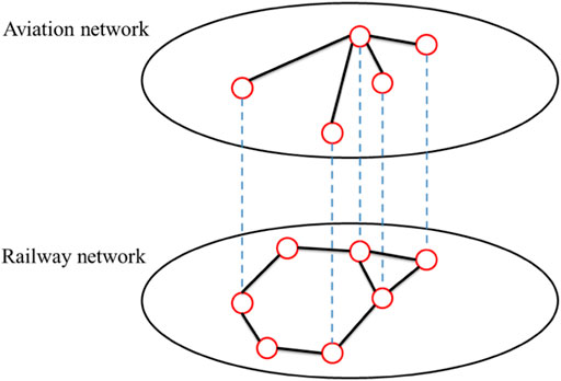
FIGURE 1. The multi-layer logistic network.

Considering that flights in the aviation network tend to be concentrated in a few airports in a heterogeneous manner [26, 27], the BA scale-free network model [28] is used to build the upper aviation layer. The main characteristic of the BA network is that it starts from the connected network with n₀ nodes. A new node is added in each time step and is connected with n existing nodes. Besides, the newly added node is more possible to connect with those nodes with higher degrees. The probability of the newly added node connecting to an existing node i is as follows

$\prod _i=\frac{k_i}{{\sum }_j{k}_j}(1)$

where k_i is the degree of node i. The BA model does not take the distance between two nodes into consideration. Therefore, the long-range edges are allowed. This fact agrees with the real aviation network. It should be noted that the BA scale-free network is not a spatial network. The positions of nodes in this layer will be determined after building the railway network.

Usually, only nearby railway nodes are connected by direct edges, and remote stations are connected through a series of nodes in between. Therefore, the modified version of random geometric graph [29, 30] is used to build the lower railway network. In this model, the longest connection distance R is defined so that two nodes with a distance longer than R cannot be connected by a direct edge. Eq. 2 is the formula for the distance between two nodes

$d_{ij}=\sqrt{{\left(x_i-x_j\right)}^2+{\left(y_i-y_j\right)}^2}(2)$

where (x_i, y_i) and (x_j, y_j) represent the geographical positions of node i and node j. On the other hand, to reflet the real case in railway network, the maximum number of edges for each node is defined, which makes sure that each node cannot have too much connections.

In the real case, it is not difficult to find that cities with airports are often equipped with railway stations, but the opposite may not be true. So, In the construction of the double-layer network, the railway network is constructed first, and the numbers of nodes is N₁. Then select N₂ nodes with largest degrees to build the aviation network. Besides, this paper focuses on the transportation process between cities, so the positions of the railway node and the airport node in the same city are assumed to be identical. In other words, the geographical positions of nodes in the double-layer network are all based on the city. In this way, the positions of nodes in the aviation network can be determined.

Basic routing model

In the logistic networks, the cost is the key issue to determine the route. The transportation cost which is composed of time cost and economic cost is defined as the edge weight in the network, as shown in the following equations

$w_{ij}^t=\left(1-m\right)\ast T_{ij}^t+m\ast E_{ij}^t(3)$

$w_{ij}^l=\left(1-m\right)\ast T_{ij}^l+m\ast E_{ij}^l(4)$

where m ∈ [0, 1] gives the proportion of economic cost in the total cost. $T_{ij}^t$ $(T_{ij}^l)$ and $E_{ij}^t$ $(E_{ij}^l)$ represent the time cost and economic cost for transporting one unit goods through the edge (i, j) in the upper aviation network (lower railway network), respectively. They can be computed as

$T_{ij}^t=\frac{d_{ij}}{V^t},T_{ij}^l=\frac{d_{ij}}{V^l},E_{ij}^t=d_{ij}\ast P^t,E_{ij}^l=d_{ij}\ast P^l(5)$

where d_ij is the length of the edge (i, j), V^t (V^l) is the traffic speed for the upper aviation network (lower railway network), and P^t (P^l) is the price for transporting unit goods to go unit distance.

After getting the cost for each edge, we can define the cost for paths between nodes i and j as the sum of cost of edges along the path. Then the path with the lowest cost is chosen to transport goods, and its cost is denoted by $w_{i\to j}^{*}$.

Cascading effect

In logistic networks, goods are transported from sources to destinations. Without loss of generality, we assign the same volume of transportation task for each pair of cities. In this way, there is load on each edge. On the other hand, each edge has a capacity, which limits the free-flow load on this edge. If its load is greater than its capacity, then congestion happens and the travel on this edge will cost extra time delay. To show this effect on the route planning, we define the congestion cost as the extra time cost when the load on an edge exceeds its capacity. It is defined as

$△T_{ij}=\left\{\begin{array}{ccc}\hfill \left(L_{ij}-C_{ij}\right)\ast T_{ij}\hfill & \hfill L_{ij}>C_{ij}\hfill & \hfill \hfill \\ \hfill 0\hfill & \hfill L_{ij}\le C_{ij}\hfill \end{array}\right.(6)$

where L_ij is the load of edge (i, j), and C_ij is the capacity of this edge.

Set the capacity of an edge to be the initial load of this edge, which means all edges work in the full load status and there is no congestion cost initially. Then, if a node (a city in the logistic network, including the airport and the railway station in this city) is removed due to failure or attack, then some paths which used to pass the removed node will be re-allocated. The re-allocation of traffic may increase the load of some edges, making them congested, and then introducing extra time cost for t he traffic passing these edges. In order to save transportation costs and obtain maximum benefits, the transportation route needs to be re-planned. We can find that this re-planning will degrade the transportation performance and increase the transportation cost on average. There will be a cascading effect during the above process. This cascading effect is different from the Motter-Lai model [31] where the cascade of node failures takes place due to overloading. In our model, the overloading will cause the increase of transportation cost rather than node failures.

In the above process, the selection of initially removed node is very important. Different initially removed node affects the final transportation cost. In this paper, we define the important node as the one so that removing this node will cause the highest increase of transportation cost.

Greedy route planning model

Here we propose a greedy route planning method to get the final routes after the initial removal of the important node. Assume one unit of goods are transported between each pair of cities. The method divides the transportation goods into M shares, and the route of each share is planned separately. The greater the value of M, the better the route planning effect. The route planning of the first share R₁ is based on the network with empty load after the initial removal of the important node. The route for the second share R₂ is planned based on the basis of the previous planning. To do that, the cost for each edge, including the extra time cost for using this edge, is calculated, and the route with the lowest cost is chosen for the transportation of share R₂ of goods. This process repeats until the route for the share R_M is planned. In the above process, each share of goods find its best route with the lowest cost based on the current traffic status. However, different share of goods, even with the same source and destination, may have different route.

Figure 2 shows the greedy route planning process under different m values. In this figure, after a node is attacked and removed, the transportation route is re-planned according to the greedy route planning method proposed above. It can be seen that when i = 1, that is, when the first share R₁ is planned, there is no overload edge in the network. And the number of overload edge after the share R_i is planned increases with i gradually.

FIGURE 2

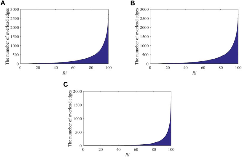
FIGURE 2. Change of the number of overload edges when the R_i share of goods is planned by using the greedy route planning model.(A) the value of m is 0.1; (B) the value of m is 0.5; (C) the value of m is 0.9.

Identification of important nodes

Traditional identification methods

In order to verify the effect of important node identification method proposed in this paper, several traditional important node identification methods are introduced here, including degree centrality (DC) [13], betweenness centrality (BC) [14], closeness centrality (CC) [15] and residual closeness centrality (RCC) [32]. Their calculation formulas are shown as follows

$DC\left(i\right)=\sum _j{a}_{ij}(7)$

$BC\left(i\right)=\sum _{i\ne s,i\ne t,s\ne t}\frac{\left(g_{st}^i\right)}{g_{st}}(8)$

$CC\left(i\right)=\sum _{j=1}^N\frac{1}{d_{ij}}(9)$

$RCC\left(i\right)=\sum _j\sum _{k\ne j}\frac{1}{2^{d_{jk}\left(-i\right)}}(10)$

In Eq. 7, a_ij is the element in the adjacency matrix; if there is a connection between nodes i and j, a_ij=1, otherwise, a_ij=0. In Eq. 8, g_st represents the number of shortest paths from node s to t, and $g_{st}^i$ represents the number of these shortest paths through node i. In Eq. 9, d_ij represents the shortest distance between nodes i and j. In Eq. 10 d_jk(−i) represents the shortest distance between nodes j and k after node i is deleted.

Proposed identification method

In the traditional identification methods, BC evaluates the load of node when the shortest path routing is adopted. However, in the logistic network, the cost, rather than only the path length, is the key for path planning. Therefore, we propose a modified version of BC, called route centrality RC, to show the load of node in the logistic network.

$RC\left(i\right)=\sum _{s\ne t}\frac{u_{s\to t}^i}{u_{s\to t}}(11)$

where u_s→t is the load transported from node s to node t, and $u_{s\to t}^i$ is the such load which goes through node i. If a node with a larger value of RC is removed, then a larger volume of load have to be re-allocated, which may have greater effect on the transportation.

Since the logistic networks are spatial networks, the position of cities plays an important role. In the traditional identification methods, CC gives a good measure how “central” a node is located in the network. However, CC counts the number of links along the shortest path to other nodes, which does not show the idea of path planning process in logistic networks. Here we propose a modified version of CC called spending centrality (SC) as

$SC\left(i\right)=\sum _{j=1}^N{w}_{i\to j}^{\ast }(12)$

It considers that the lower the cost of transporting goods to other nodes, the more important and central the node is in the network. Specifically, when the goods can not be transported from node i to node j, i.e., there is no path from i to j, then the cost $w_{i\to j}^{*}=0$.

Finally, the identification method RSC in this paper is proposed based on the above two modified methods RC and SC, as shown in the following equation.

$RSC\left(i\right)=\frac{RC\left(i\right)}{max\left(RC\right)}-\frac{SC\left(i\right)}{max\left(SC\right)}(13)$

The basic idea is that the more frequently a node is used in the initial transport route, and the lower the cost of transporting goods from it to other nodes, the more important the node is.

Network performance index

For the logistic network, the failure of a city’s railway station and airport does not lead to the failure of others. So, for the transportation model in this paper, the failure of network nodes will only cause the redistribution of load in the network, resulting in congestion. Therefore, the traditional network performance indexes, such as the relative size of the largest connected component [31] and network efficiency [33], are not suitable for the study in this paper.

After the initial failure, the congestion will lead to the increase of transportation cost. The failure of the most important node makes the cost increase the most, and the failure of the most unimportant node makes the cost increase the least. Therefore, the change of cost is a good measure of performance in our model. Use cost_before and cost_after to denote the total cost for transporting one unit of goods between each pair of nodes in the network before and after the initial failure, respectively. The performance index is the difference between them, defined as

$\mathrm{\Delta }cost=\frac{cos{t}_{\mathit{after}}-cos{t}_{\mathit{before}}}{cos{t}_{\mathit{before}}}(14)$

Simulations

Network parameters setting

In this paper, we consider the logistic system of 500 cities. One railway station is allocated in a city, but only 200 cities out of 500 have airport. Therefore, a multi-layer logistic network with 200 nodes in the upper aviation network and 500 nodes in the lower railway network is constructed. The upper network is a BA network with an average degree of 10. The edges in this network are highly concentrated, that is, a small number of nodes have most of the links in the network. And the nodes of the aviation network are coupled with the nodes of the lower railway network according to the degree. The lower railway network is a modified random geometric graph, and whether there is an edge between nodes depends on the distance, and its average degree is approximately 10. Referring to the speed and transportation prices between flight and trains in real life, the time cost of the upper aviation network in the unit distance is set to be 1/3 of that of the lower railway network, and the economic cost is 5 times of that in the railway network.

Simulation results

Figure 3 shows how the transportation cost for increasing each share of goods in the planning route process changes when the most important node is removed as the initial attack. To make the comparison fair, the cost is normalized by

$cos{t}_i=\frac{\left(p_i\right)}{\left(p_1\right)}(15)$

where p_i represents the transportation cost for increasing share R_i of goods into the nework. We can find that all the curves in the figure are increasing, indicating the congestion status becomes more and more severe in the greedy route planning process. Among different important node identification methods, our proposed RSC makes the biggest trouble as removing the most important node based on this method results in the highest cost for the transportation in the rest network.

FIGURE 3

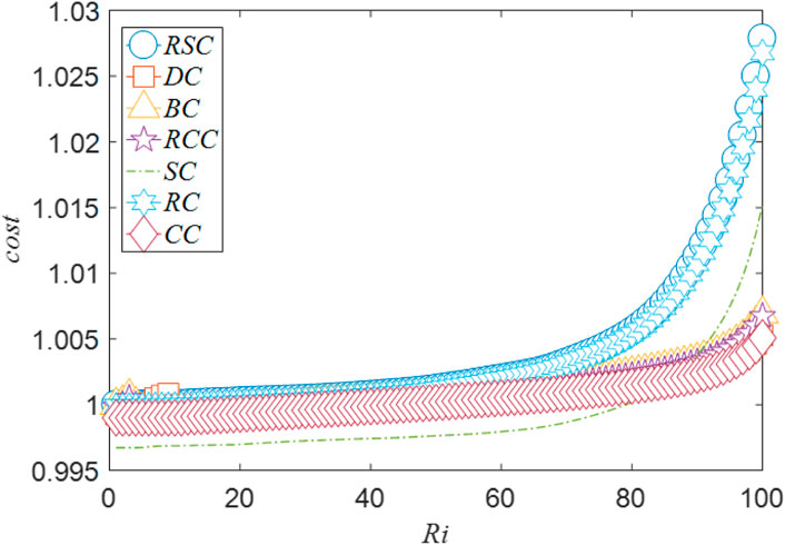
FIGURE 3. The cost for increasing a share of goods in the route planning process, after the removal of the most important node identified by different identification methods. m = 0.5. Each point is the average of 10 runs.

On the contrary, Figure 4 shows the transport cost for each share of goods in the route planning process when the least important node is removed as the initial attack. All the curves in Figure 4 are horizontal, which is very different from Figure 3. This is because the effect of the least important node is so weak that its removal does not cause any congestion. Therefore, the cost does not change for each share of goods. Among all the curves, our proposed method RSC achieves the lowest cost, indicating that it finds the least important node effectively.

FIGURE 4

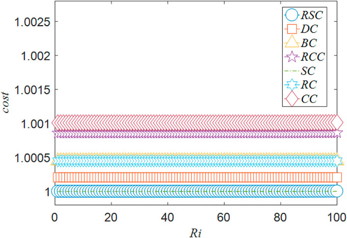
FIGURE 4. The cost for increasing a share of goods in the route planning process, after the removal of the least important node identified by different identification methods. m = 0.5. Each point is the average of 10 runs.

More interestingly, the above conclusion holds when the proportion of economic cost m changes. Figure 5 shows the change of total cost after the most important node is removed. Here the change of total cost is define as the difference between the total costs after and before the removal of the most important node. It can be seen that under different m, RC and RSC curves are higher than other curves, that is, RC and RSC have better ability to identify important node than other methods. So, for the first evaluation perspective, RC and RSC identification methods are clearly better. Figure 6 shows the change of the total cost after the least important node is removed. In the figure, SC and RSC curves are lower than other curves, indicating that these two methods can efficiently identify the least important nodes in the network. Combining the above two aspects together, the proposed RSC method outperforms in finding both the most important node and the least important node.

FIGURE 5

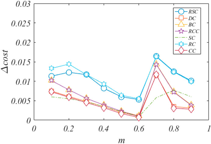
FIGURE 5. The change of total transportation cost after the removal of the most important node. Here Δcost is the difference between the total costs after and before the removal of the most important node. Each point is the average of 10 runs.

FIGURE 6

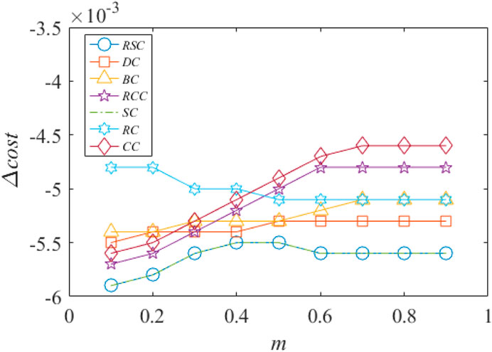
FIGURE 6. The change of total transportation cost after the removal of the least important node. Here Δcost is the difference between the total costs after and before the removal of the least important node. Each point is the average of 10 runs.

Conclusion

Identification of the important node in networks is a key issue to analyze the performance of networks. Previous identification methods are mainly designed for single network, and their performance may be doubtable in multi-layer networks. In this paper, a new identification method is proposed for a two-layer logistic network. In this scenario, the removal of the most important node can increase the cost of transportation the most. Our proposed method considers the load on the node and the cost for the route from this node to other nodes. The simulation results indicate that our method can find both the most important node and least important node effectively.

Data availability statement

The original contributions presented in the study are included in the article/supplementary material, further inquiries can be directed to the corresponding author.

Author contributions

All authors listed have made a substantial, direct, and intellectual contribution to the work and approved it for publication.

Funding

This work was supported by the Laboratory of Science and Technology on Integrated Logistics Support, China (Grant No. 6142003190101).

Conflict of interest

The authors declare that the research was conducted in the absence of any commercial or financial relationships that could be construed as a potential conflict of interest.

Publisher’s note

All claims expressed in this article are solely those of the authors and do not necessarily represent those of their affiliated organizations, or those of the publisher, the editors and the reviewers. Any product that may be evaluated in this article, or claim that may be made by its manufacturer, is not guaranteed or endorsed by the publisher.

References

1. Santiago SG, Felipe BM, Agustina C. Understanding the effect of traffic congestion on accidents using big data. Sustainability (2021) 13:7500. doi:10.3390/su13137500

CrossRef Full Text | Google Scholar

2. Zhang M, Chen S, Sun L, Du W, Cao X. Characterizing flight delay profiles with a tensor factorization framework. Engineering (2021) 7:465–72. doi:10.1016/j.eng.2020.08.024

CrossRef Full Text | Google Scholar

3. Wang W, Cai K, Du W, Wu X, Tong L, Zhu X, et al. Analysis of the Chinese railway system as a complex network. Chaos Solitons & Fractals (2020) 130:109408. doi:10.1016/j.chaos.2019.109408

CrossRef Full Text | Google Scholar

4. Albert R, Jeong H, Barabási AL. Error and attack tolerance of complex networks. Nature (2000) 406:378–82. doi:10.1038/35019019

PubMed Abstract | CrossRef Full Text | Google Scholar

5. Council NAER, Anderson RN. August 14, 2003 blackout: Nerc actions to prevent and mitigate the impacts of future cascading blackouts. Atlanta, Georgia: North American Electric Reliability Council (2004). p. 10.

Google Scholar

6. Newman ME. Network: An introduction. Oxford, UK: Oxford Univeristy Press (2010).

Google Scholar

7. Boccaletti S, Latora V, Moreno Y, Chavez M, Hwang DU. Complex networks: Structure and dynamics. Phys Rep (2006) 424:175–308. doi:10.1016/j.physrep.2005.10.009

CrossRef Full Text | Google Scholar

8. Boccaletti S, Bianconi G, Criado R, del Genio C, Gómez-Gardeñes J, Romance M, et al. The structure and dynamics of multilayer networks. Phys Rep (2014) 544:1–122. doi:10.1016/j.physrep.2014.07.001

PubMed Abstract | CrossRef Full Text | Google Scholar

9. Barabasi AL. Network science. Cambridge: Cambridge University Press (2016).

Google Scholar

10. Xia Y, Small M, Wu J. Introduction to focus issue: Complex network approaches to cyber-physical systems. Chaos (2019) 29:093123. doi:10.1063/1.5126230

PubMed Abstract | CrossRef Full Text | Google Scholar

11. Jiang J, Xia Y, Xu S, Shen H, Wu J. An asymmetric interdependent networks model for cyber-physical systems. Chaos (2020) 30:053135. doi:10.1063/1.5139254

PubMed Abstract | CrossRef Full Text | Google Scholar

12. Dong G, Wang F, Shekhtman LM, Danziger MM, Fan J, Du R, et al. Optimal resilience of modular interacting networks. Proc Natl Acad Sci U S A (2021) 118:e1922831118. doi:10.1073/pnas.1922831118

PubMed Abstract | CrossRef Full Text | Google Scholar

13. Bonacich P. Factoring and weighting approaches to status scores and clique identification. J Math Sociol (1972) 2:113–20. doi:10.1080/0022250X.1972.9989806

CrossRef Full Text | Google Scholar

14. Freeman LC. A set of measures of centrality based on betweenness. Sociometry (1977) 40:35–41. doi:10.2307/3033543

CrossRef Full Text | Google Scholar

15. Freeman LC. Centrality in social networks conceptual clarification. Social networks (1978) 1:215–39. doi:10.1016/0378-8733(78)90021-7

CrossRef Full Text | Google Scholar

16. Lordan O, Sallan JM, Simo P, Gonzalez-Prieto D. Robustness of the air transport network. Transportation Res E: Logistics Transportation Rev (2014) 68:155–63. doi:10.1016/j.tre.2014.05.011

CrossRef Full Text | Google Scholar

17. Yang Y, Liu Y, Zhou M, Li F, Sun C. Robustness assessment of urban rail transit based on complex network theory: A case study of the beijing subway. Saf Sci (2015) 79:149–62. doi:10.1016/j.ssci.2015.06.006

CrossRef Full Text | Google Scholar

18. Liu P, Li L, Fang S, Yao Y. Identifying influential nodes in social networks: A voting approach. Chaos Solitons & Fractals (2021) 152:111309. doi:10.1016/j.chaos.2021.111309

CrossRef Full Text | Google Scholar

19. Liu P, Li L, Fang S, Yao Y, Deng Y. Identifying influential spreaders by weight degree centrality in complex networks. Chaos Solitons & Fractals (2016) 86:1–7. doi:10.1016/j.chaos.2016.01.030

CrossRef Full Text | Google Scholar

20. Wen T, Jiang W. Identifying influential nodes based on fuzzy local dimension in complex networks. Chaos Solitons & Fractals (2019) 119:332–42. doi:10.1016/j.chaos.2019.01.011

CrossRef Full Text | Google Scholar

21. Zhao J, Wang Y, Deng Y. Identifying influential nodes in complex networks from global perspective. Chaos Solitons & Fractals (2020) 133:109637. doi:10.1016/j.chaos.2020.109637

CrossRef Full Text | Google Scholar

22. Yu E, Wang Y, Fu Y, Chen D, Xie M. Identifying critical nodes in complex networks via graph convolutional networks. Knowledge-Based Syst (2020) 198:105893. doi:10.1016/j.knosys.2020.105893

CrossRef Full Text | Google Scholar

23. Ye W, Liu Z, Pan L. Who are the celebrities? Identifying vital users on sina weibo microblogging network. Knowledge-Based Syst (2021) 231:107438. doi:10.1016/j.knosys.2021.107438

CrossRef Full Text | Google Scholar

24. Zhu L, Xia Y, Bai G, Fang Y. Key repairing node identification in double-layer logistic networks. Front Phys (2022) 10:105893. doi:10.3389/fphy.2022.919455

CrossRef Full Text | Google Scholar

25. Liu T, Bai G, Tao J, Zhang Y, Fang Y, Xu B. Modeling and evaluation method for resilience analysis of multi-state networks. Reliability Eng Syst Saf (2022) 2022:108663. doi:10.1016/j.ress.2022.108663

CrossRef Full Text | Google Scholar

26. Hossain MM, Alam S. A complex network approach towards modeling and analysis of the australian airport network. J Air Transport Manage (2017) 60:1–9. doi:10.1016/j.jairtraman.2016.12.008

CrossRef Full Text | Google Scholar

27. Du W, Zhou X, Lordan O, Wang Z, Zhao C, Zhu Y. Analysis of the Chinese airline network as multi-layer networks. Transportation Res Part E: Logistics Transportation Rev (2016) 89:108–16. doi:10.1016/j.tre.2016.03.009

CrossRef Full Text | Google Scholar

28. Barabási AL, Albert R. Emergence of scaling in random networks. Science (1999) 286:509–12. doi:10.1126/science.286.5439.509

PubMed Abstract | CrossRef Full Text | Google Scholar

29. Barthélemy M. Spatial networks. Phys Rep (2011) 499:1–101. doi:10.1016/j.physrep.2010.11.002

CrossRef Full Text | Google Scholar

30. Liang Y, Xia Y, Yang X. Hybrid-radius spatial network model and its robustness analysis. Physica A: Stat Mech its Appl (2022) 591:126800. doi:10.1016/j.physa.2021.126800

CrossRef Full Text | Google Scholar

31. Motter AE, Lai YC. Cascade-based attacks on complex networks. Phys Rev E (2002) 66:065102. doi:10.1103/physreve.66.065102

PubMed Abstract | CrossRef Full Text | Google Scholar

32. Latora V, Marchiori M. Efficient behavior of small-world networks. Phys Rev Lett (2001) 87:198701. doi:10.1103/PhysRevLett.87.198701

PubMed Abstract | CrossRef Full Text | Google Scholar

33. Liang Y, Xia Y, Yang X, Rapisarda A. Efficiency of scale-free networks: Error and attack tolerance. Physica A: Stat Mech its Appl (2003) 320:622–42. doi:10.1016/S0378-4371(02)01545-5

CrossRef Full Text | Google Scholar