A second-order non-local model for granular flows

1 Introduction

Granular materials (sand, gravel, coal, salt, rice, wheat, pills, etc.) are essential to our lives and used in diverse scientific fields and industries. Although the microscopic interactions between grains are simple, the macroscopic mechanical properties of granular flows arising from these simple interactions are surprisingly complex and still subject to debate.

One hypothetical way to write the constitutive equation for granular flows is to assume that the deviatoric stress is codirectional to the strain rate tensor D:

$\mathit{\sigma }=-P\mathit{I}+\tau \frac{2}{\dot{\gamma }}\mathit{D}(1)$

where σ is the stress tensor, P is the pressure, $\dot{\gamma }$ is the shear rate, and τ is the shear stress. Let us call this model the first-order model because this model ignores higher-order velocity gradient terms which we will consider later in this article. Recent achievements in granular rheology have used this first-order model and expressed τ with kinematic variables. One of them is the μ(I) rheology [1–3], which has accurately described homogeneous flows (simple shear flows). In this model, the shear stress is obtained from a one-to-one relation between two local dimensionless variables: the shear-to-normal stress ratio μ ≡ τ/P and the inertial number $I\equiv \dot{\gamma }/\sqrt{P/{\rho }_s{d}^2}$ for 3D grains where $\dot{\gamma }$ is the shear strain rate, ρ_s is the solid grain density, and d is the mean diameter of the grains. The μ(I) rheology claims that the shear rate vanishes if μ is smaller than a bulk friction coefficient μ_s, and I monotonically increases as μ increases for μ > μ_s. However, in the dense regime of inhomogeneous flows, many researchers have observed “non-local” phenomena where this one-to-one relation between local μ and I breaks down. For example, creeping flows characterized by exponentially-decaying velocity profiles have been observed in regions with μ < μ_s [1, 4–8]. The left contour plot in Figure 1 shows an example of the creeping flows: The downstream velocity in a rough-walled inclined chute flow decays exponentially with depth, disobeying the μ(I) rheology.

FIGURE 1

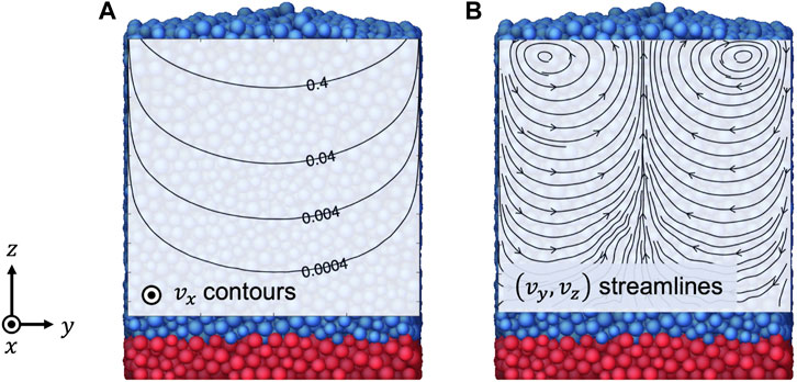
FIGURE 1. Snapshot from DEM simulation of granular flow in a chute with an inclination angle of tan⁻¹(0.50). Contour plot in (A) shows downstream velocity v_x which decreases exponentially with depth (creeping flow). The unit is $\sqrt{Gd}$ where G is gravity and d is the grain diameter. Streamlines in (B) illustrate transverse velocity (v_y, v_z) which is small but not zero (secondary flow). Our goal is to build a second-order non-local model that can explain both flows. Details of the simulation can be found in Section 3.1.

To describe this non-locality, several first-order models have introduced a diffusing scalar field that fluidizes (softens) the material. The definition of the diffusing field depends on the model. Some models have utilized the population of shear transformation zones [9–11]. The partial fluidization theory proposed by Aranson and Tsimring [12, 13]; [14] uses the average ratio of “solid contacts” as the diffusing scalar field. Inspired by a plastic flow model for soft glassy materials [15, 16], Kamrin and colleagues [17–19] have proposed the non-local granular fluidity (NGF) model that accurately describes many different inhomogeneous flows. In the NGF model, the diffusing parameter or “fluidity” is defined as the shear rate-to-μ ratio $(g\equiv \dot{\gamma }/\mu )$ and follows an empirical diffusion-reaction equation. Later, Zhang and Kamrin [20] found that the fluidity divided by the velocity fluctuations δv can be approximated as a function of the packing fraction ϕ alone: gd/δv ≈ F(ϕ). This relation is also in line with the kinetic theory of granular flows [21–24], which mathematically derives the constitutive equations using the Chapman-Enskog method. The pressure and the shear stress are predicted as P = ρ_sF₁(ϕ)T and $\tau ={\rho }_s{F}_2(\varphi )\sqrt{T}\dot{\gamma }d$ respectively where T ≡ δv²/D is “granular temperature” for the space dimension D, and F₁(ϕ) and F₂(ϕ) are dimensionless functions calculated from the radial distribution function. The shear-to-normal stress ratio can be written as $\mu =\left[F_2(\varphi )/F_1(\varphi )\right]\dot{\gamma }d/\sqrt{T}$ which is similar to Zhang and Kamrin’s fluidity expression.

Based on the fact that the fluidity is related to the velocity fluctuations, Kim and Kamrin [25] have recently proposed a first-order non-local model removing rheological dependence on ϕ. Using discrete element method (DEM) simulations in steady-state planar shear flows, a simpler constitutive relation between μ, I, and a dimensionless granular temperature Θ ≡ ρ_sT/P has been identified:

$\mu ={\mathrm{\Theta }}^{-p}f\left(I\right)(2)$

where the exponent p is approximately 1/6 for spheres in 3D and f(I) is a monotonically increasing function of I and its details depends on the material properties such as surface friction. This μ(I, Θ) relation has successfully explained the non-locality of granular flows, bridging the softening effect of granular temperature in the kinetic theory and the fluidity field in the NGF model.

However, the first-order model lacks the ability to explain a group of phenomena in granular flows. One example is a bulging surface of a channel flow. When a granular material is released steadily down an inclined plane with rough side walls, the surface of the flowing region becomes convex upward [26–29]. Another phenomenon that the first-order model cannot predict is the secondary flow. In the cylindrical Couette geometry under gravity, non-zero velocities in the radial and the gravity directions (transverse directions) have been observed and named “secondary flow” in the sense that this flow is relatively slow and perpendicular to the primary flow direction [30–33]. The right streamline plot in Figure 1 illustrates an example of the secondary flow: an inclined chute flow has non-zero transverse velocities perpendicular to the downstream direction. The anomalous shear stress observed in the plane of the secondary flows [30, 34] also cannot be accounted for in the first-order model. These phenomena occur in the presence of broken codirectionality, where the deviatoric stress and strain rate tensors are not proportional. Many other studies have also found that granular flows exhibit broken codirectionality in the form on non-zero normal stress differences [35–45] or broken coaxiality where the principal axes of the stress and strain rate tensors are not aligned [45–47]. Therefore, the constitutive equation needs to be corrected beyond the codirectionality hypothesis (Eq. 1) to achieve higher accuracy.

In the present study, we propose a non-local second-order fluid model to cover both non-locality and broken codirectionality of three-dimensional granular flows. As previous researchers have suggested [29, 45, 48], we assume steadily flowing granular fluids are incompressible non-Newtonian fluids and adopt the tensor form of the second-order fluid, also known as the Rivlin-Ericksen fluid of second grade, as the constitutive equation. In this second-order model, three functions should be calibrated. The major difference from the previous second-order models is that we take into account the dimensionless granular temperature Θ as well as I in the calibration because we know that the first-order model’s μ depends both on I and Θ. For the calibration, planar shear flows of frictional spheres are simulated using the discrete element method (DEM). We separately measure the three normal stresses, which are required to calculate the model parameters for the quadratic terms. It also allows us to examine the first and second normal stress differences.

Furthermore, we validate our non-local second-order model in a more complex geometry. Using the functions calibrated from the planar shear tests, we run the finite difference method (FDM) simulations of rough-walled inclined chute flow (Figure 1) with four different slope angles. We compare the FDM predictions to the DEM data to demonstrate that our second-order model can correctly predict the secondary flows and the stress fields as well as the primary creeping flows.

2 Model calibration: Planar shear flows

2.1 Second-order model

Following previous studies [29, 45, 48], we assume that a flowing granular material behaves like a second-order fluid where the stress tensor is of the form:

$\mathit{\sigma }=a_0{\mathit{A}}_0+a_1{\mathit{A}}_1+a_2{\mathit{A}}_1^2+a_3{\mathit{A}}_2(3)$

where A_n are called the nth order Rivlin-Ericksen tensors and a_n are scalar parameters. The Rivlin-Ericksen tensors are given by the recurrence relation

$\begin{array}{cc}\hfill {\mathit{A}}_0& =\mathit{I}\hfill \\ \hfill {\mathit{A}}_n& =\frac{D{\mathit{A}}_{n-1}}{Dt}+{\mathit{A}}_{n-1}\mathit{L}+{\mathit{L}}^T{\mathit{A}}_{n-1}\text{for\hspace{0.17em}}n=\mathrm{1,2},\dots \hfill \end{array}(4)$

where L = ∇v is the velocity gradient tensor. In steady state, this relation yields A₁ = 2D and A₂ = 4D² + 2(DW − WD) where D = (L + L^T)/2 is the strain rate tensor and W = (L − L^T)/2 is the spin tensor. Therefore, we can rewrite Eq. 3 as

$\begin{array}{cc}\hfill \mathit{\sigma }=P& \left[-\mathit{I}+{\mu }_1\frac{2}{\dot{\gamma }}\left(\mathit{D}-\frac{1}{3}\mathrm{t}\mathrm{r}\left(\mathit{D}\right)\mathit{I}\right)-{\mu }_2{\left(\frac{2}{\dot{\gamma }}\right)}^2\left({\mathit{D}}^2-\frac{1}{3}\mathrm{t}\mathrm{r}\left({\mathit{D}}^2\right)\mathit{I}\right)\right.\hfill \\ \hfill & \left.-{\mu }_3{\left(\frac{2}{\dot{\gamma }}\right)}^2\left(\mathit{D}\mathit{W}-\mathit{W}\mathit{D}\right)\right]\hfill \end{array}(5)$

where the scalar parameters μ₁, μ₂, and μ₃ play the same role as those in Srivastava et al. [45]. Since all but the identity tensor in the above expression are deviatoric, the pressure P represents the hydrostatic pressure P ≡ − tr σ/3. Our definition of the shear rate $\dot{\gamma }\equiv \sqrt{2{\mathit{D}}^{\prime }:{\mathit{D}}^{\prime }}$ is double the $\dot{\gamma }$ used in [45]. The tensor inner product is defined by M: N = ∑_i,jM_ijN_ij for arbitrary tensors M and N. In our sign convention, compressive normal stresses are negative.

In Srivastava et al. [45], μ₁, μ₂, and μ₃ were assumed to depend only on I. However, the previous non-local first-order model by Kim and Kamrin [25], which is equivalent to the case of μ₂ = μ₃ = 0, suggests that μ₁ depends on both I and Θ. It suggests that μ₂ and μ₃ may also be affected by Θ in inhomogeneous flows. In this work, we run various planar shear flows using DEM simulations to find the expressions for μ₁, μ₂, and μ₃ in terms of I and Θ. Using our calibrated parameters, we check the predictive capability of our model in chute flows with different inclination angles.

2.2 Methods

2.2.1 DEM simulation settings for planar shear flows

In order to identify the parameters in the second-order model, we use LAMMPS (Large-scale Atomic/Molecular Massively Parallel Simulator), which implements the discrete element method (DEM), to simulate many different homogeneous and inhomogeneous planar shear flows of 3D frictional spheres. The grain diameter d_i is set to be uniformly distributed from 0.8d to 1.2d to prevent crystallization. When we calculate I, the local average diameter is used. The mass of the grains is determined as $m_i=\frac{4}{3}\pi {(d_i/2)}^3{\rho }_s$, which distributes around $m\equiv \frac{4}{3}\pi {(d/2)}^3{\rho }_s$. For the contact forces, we use the standard spring-dashpot model introduced by Cundall and Strack [49] with Coulomb friction. This model has been used in many previous studies, such as to study simple shear flows in 2D [2] and various inhomogeneous flows in 2D [5, 17, 50, 51] and 3D [20, 25]. In this model, the normal force is given by F_n = k_nδ_n − γ_nv_n (repulsive) where k_n is the normal elastic constant, δ_n is the normal component of the contact displacement, γ_n is the damping coefficient, and v_n is the normal component of the relative velocity. We use k_n = 2.63 N/m × 10⁵ N/m, d = 0.0008 m, and ρ_s = 2500 kg/m³ which can be considered when reading the pressure data in Figure 13. The tangential force is given by F_t = −k_tδ_t for |k_tδ_t| < μ_pF_n and F_t = −μ_pF_n × (δ_t/|δ_t|) for |k_tδ_t| > μ_pF_n where μ_p = 0.4 is the surface friction coefficient and δ_t is the tangential component of the contact displacement obtained by integrating tangential relative velocity during the collision. The minus sign indicates the tangential force is pointing in the direction of decreasing δ_t. The tangential elastic constant k_t is set to be 2/7 of k_n such that the frequencies of normal and tangential contact oscillations are similar [43]. To simulate hard particles, the stiffness number k_n/Pd is kept larger than 10⁵. The damping coefficient for the restitution coefficient ϵ and the effective mass of collision m_eff, which is approximately m/2, is calculated as ${\gamma }_n=\sqrt{4m_{\text{eff}}{k}_n/(1+{(\pi /\ln ϵ)}^2)}$ [2, 51]. We set ϵ = 0.24 to match with Kim and Kamrin [25]. The choice of k_t and ϵ is known to have little impact on the flow behavior in the case of dense flows of hard particles, as reported in [2, 37, 52]. The simulation time step is set to be 6% of the binary collision time ${\tau }_c=\pi \sqrt{\frac{m}{2k_n}\left(1+{(\ln ϵ/\pi )}^2\right)}$ which is half the period of an underdamped oscillator made of the two identical grains.

As in Kim and Kamrin [25], we test simple shear flows (Figure 2A), shear flows under gravity (Figure 2B), flows in vertical and tilted chutes (θ = 90° and 60° in Figure 2C), and “concave flows” (Figure 2D). The concave flow is named so because the plot of the shear rate against height becomes concave upward due to the outward body force ${\vec{F}}_z=(m_{i}G/d)(z-z_0)\widehat{z}$ for the midpoint of the system z₀. G is a constant. The horizontal length and depth of the system are L_x = 20d and L_y = 16d respectively and the side boundaries are set to be periodic. Following previous studies [2, 5, 20, 25, 50, 51], we move the top wall in the z-direction to maintain the top-wall pressure P_wall. The horizontal wall velocity V_wall is set to be constant. More detailed DEM simulation conditions are in the Supplementary Material.

FIGURE 2

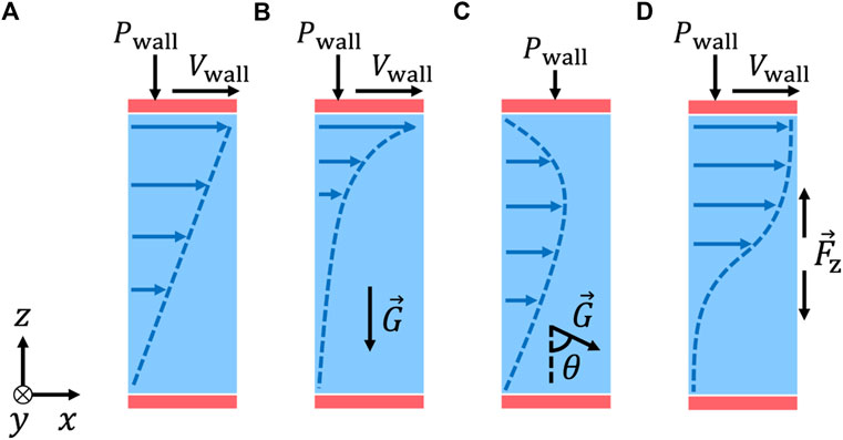
FIGURE 2. Schematic diagrams of planar shear flows used for model calibration in Section 2: (A) simple shear, (B) shear with gravity, (C) chute flows (θ = 60° and 90°), and (D) concave flows. Red rectangles represent wall particles whose velocities are set to form rigid walls. Dashed lines indicate velocity profiles. x is the flow direction, y is the vorticity direction, and z is the velocity gradient direction.

The continuum variables at each height are obtained by coarse graining, in the same way as [25]. The instantaneous packing fraction at time t can be calculated as

$\varphi \left(z_k,t\right)=\frac{{\sum }_i{A}_{ki}}{A}(6)$

where A is the area of the horizontal plane and A_ki is the cross-sectional area between the ith particle and the plane of z = z_k. We kept the interval of z_k less than 0.5d. The macroscopic velocity field can be calculated as

$\vec{v}\left(z_k,t\right)=\frac{{\sum }_i{A}_{ki}{\vec{v}}_i\left(t\right)}{{\sum }_i{A}_{ki}}(7)$

where ${\vec{v}}_i$ is the velocity of the ith particle. We define the instantaneous granular temperature tensor as

$\mathbf{T}\left(z_k,t\right)=\frac{{\sum }_i{A}_{ki}\left[\delta {\vec{v}}_i\left(t\right)\otimes \delta {\vec{v}}_i\left(t\right)\right]}{{\sum }_i{A}_{ki}}(8)$

where $\delta {\vec{v}}_i(t)={\vec{v}}_i(t)-\vec{v}(z_k,t)$ is the instantaneous velocity fluctuation of the ith particle. The instantaneous stress is

$\mathit{\sigma }\left(z_k,t\right)={\mathit{\sigma }}^K\left(z_k,t\right)+\frac{{\sum }_i{A}_{ki}{\mathit{\sigma }}_i\left(t\right)}{A}(9)$

where σ_i is the contact stress of the ith particle, and σ^K = −ρ_sϕ T is the kinetic stress [43]. The specific formula for σ_i is

${\mathit{\sigma }}_i=\frac{1}{V_i}\sum _{j\ne i}\frac{1}{2}{\vec{r}}_{ij}\otimes {\vec{f}}_{ij}(10)$

where V_i is the volume of the ith particle, ${\vec{r}}_{ij}$ is the displacement from the center of the ith particle to the center of the jth particle, and ${\vec{f}}_{ij}$ is the interaction force exerted on the ith particle by the jth particle. For one particle, the stress tensor may not be symmetric. However, if a sufficient number of particles are averaged, the coarse-grained stress tensor becomes symmetric as shown by [53]. We choose $(T_{yy}+T_{zz})/2=(\delta v_y^2+\delta v_z^2)/2$ as the granular temperature T because for some flows, T_xx is measured quite differently from the other diagonal elements. The ratios between diagonal elements of the granular temperature in the inclined chute flow can be found in the Supplementary Material. These coarse-grained fields are averaged over time once the flow reaches a steady state. We cut off the data where total local shear is less than 1 or the distance from the walls is less than 3d to include enough configurations and exclude the wall effect.

2.2.2 Calculation of model parameters in planar shear flows

The second-order model parameters μ₁, μ₂, and μ₃ can be calculated from the measured stress tensor and velocity gradient tensor in the DEM planar shear flows (Figure 2). By symmetry, both homogeneous and inhomogeneous flows have negligible mean v_y and v_z and the mean v_x changes only in the z-direction. Therefore, the velocity gradient tensor has only one non-zero component: $L_{xz}=v_{x,z}\equiv \frac{\partial v_x}{\partial z}$ which can vary depending on the height. With its magnitude $\dot{\gamma }$, the inertial number can be obtained as $I=\dot{\gamma }/\sqrt{P/{\rho }_s{d}^2}$. By definition, the symmetric strain rate tensor D and the spin tensor W are

$\mathit{D}=\left(\begin{array}{ccc}\hfill 0\hfill & \hfill 0\hfill & \hfill v_{x,z}/2\hfill \\ \hfill 0\hfill & \hfill 0\hfill & \hfill 0\hfill \\ \hfill v_{x,z}/2\hfill & \hfill 0\hfill & \hfill 0\hfill \end{array}\right)\text{and}\mathit{W}=\left(\begin{array}{ccc}\hfill 0\hfill & \hfill 0\hfill & \hfill v_{x,z}/2\hfill \\ \hfill 0\hfill & \hfill 0\hfill & \hfill 0\hfill \\ \hfill -v_{x,z}/2\hfill & \hfill 0\hfill & \hfill 0\hfill \end{array}\right)(11)$

respectively. Using

${\mathit{D}}^2-\frac{\mathrm{t}\mathrm{r}\left({\mathit{D}}^2\right)}{3}\mathit{I}=\frac{{v_{x,z}}^2}{12}\left(\begin{array}{ccc}\hfill 1\hfill & \hfill 0\hfill & \hfill 0\hfill \\ \hfill 0\hfill & \hfill -2\hfill & \hfill 0\hfill \\ \hfill 0\hfill & \hfill 0\hfill & \hfill 1\hfill \end{array}\right)(12)$

and

$\mathit{D}\mathit{W}-\mathit{W}\mathit{D}=\frac{{v_{x,z}}^2}{2}\left(\begin{array}{ccc}\hfill -1\hfill & \hfill 0\hfill & \hfill 0\hfill \\ \hfill 0\hfill & \hfill 0\hfill & \hfill 0\hfill \\ \hfill 0\hfill & \hfill 0\hfill & \hfill 1\hfill \end{array}\right),(13)$

we can express the stress tensor (Eq. 5) as

$\mathit{\sigma }=P\left(\begin{array}{ccc}\hfill -\left(1+\frac{1}{3}{\mu }_2-2{\mu }_3\right)\hfill & \hfill 0\hfill & \hfill {\mu }_1\frac{v_{x,z}}{\dot{\gamma }}\hfill \\ \hfill 0\hfill & \hfill -\left(1-\frac{2}{3}{\mu }_2\right)\hfill & \hfill 0\hfill \\ \hfill {\mu }_1\frac{v_{x,z}}{\dot{\gamma }}\hfill & \hfill 0\hfill & \hfill -\left(1+\frac{1}{3}{\mu }_2+2{\mu }_3\right)\hfill \end{array}\right).(14)$

Because $v_{x,z}/\dot{\gamma }=1$ for v_x,z > 0 and $v_{x,z}/\dot{\gamma }=-1$ for v_x,z < 0, the sign of σ_xz is determined by the sign of v_x,z while the magnitude of σ_xz is μ₁P in either case. We can see that the second-order model parameters μ₂ and μ₃ introduce differences between the normal stress components. Inversely, the three parameters can be extracted from the stress measurement using the fact that the basis tensors I, $\left(\mathit{D}-\frac{1}{3}\mathrm{t}\mathrm{r}(\mathit{D})\mathit{I}\right)$, $\left({\mathit{D}}^2-\frac{1}{3}\mathrm{t}\mathrm{r}({\mathit{D}}^2)\mathit{I}\right)$, and $\left(\mathit{D}\mathit{W}-\mathit{W}\mathit{D}\right)$ are orthogonal to each other under the tensor inner product:

$\begin{array}{cc}\hfill {\mu }_1& =\frac{1}{\dot{\gamma }P}\mathit{\sigma }:\mathit{D}=\frac{{\sigma }_{xz}}{P}\frac{v_{x,z}}{\dot{\gamma }}=\frac{|{\sigma }_{xz}|}{P}\hfill \\ \hfill {\mu }_2& =\frac{6}{{\dot{\gamma }}^{2}P}\mathit{\sigma }:\left({\mathit{D}}^2-\frac{\mathrm{t}\mathrm{r}{\mathit{D}}^2}{3}\mathit{I}\right)=-\frac{{\sigma }_{xx}+{\sigma }_{zz}-2{\sigma }_{yy}}{2P}\hfill \\ \hfill {\mu }_3& =\frac{1}{2{\dot{\gamma }}^{2}P}\mathit{\sigma }:\left(\mathit{D}\mathit{W}-\mathit{W}\mathit{D}\right)=\frac{{\sigma }_{xx}-{\sigma }_{zz}}{4P}\hfill \end{array}(15)$

with the assumption that the flow follows the second-order fluid equation (Eq. 5).

2.3 Model calibration results from DEM planar shear flows

2.3.1 Normal stress ratio measurement

The ratios between the coarse-grained normal stresses from the planar shear tests are plotted in Figure 3. Figure 3A shows that the normal stress in the flow direction σ_xx is nearly the same as the normal stress in the velocity gradient direction σ_zz for the low I regime (I < 0.1). As I increases beyond 0.1, the magnitude of σ_xx becomes larger than the magnitude of σ_zz and their ratio σ_xx/σ_zz keeps increasing. This behavior is similar to previous findings in 2D and 3D granular systems [35, 36, 38–40, 43, 45]. On the other hand, the normal stress in the vorticity direction σ_yy is spread between 85% and 95% of σ_zz for I < 0.1. As I increases beyond 0.1, the ratio becomes even smaller as shown in Figure 3B. This is in line with previous observations [37, 43, 45].

FIGURE 3

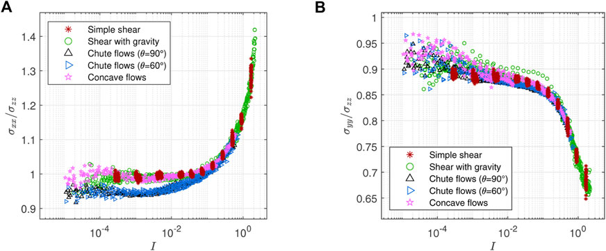
FIGURE 3. Normal stress ratios in planar shear tests: (A) σ_xx/σ_zz is near 1 for I < 0.1 and increases rapidly as I increases for I > 0.1. (B) σ_yy/σ_zz is spread between 0.85 and 0.95 for I < 0.1 and becomes even smaller as I increases for I > 0.1.

2.3.2 μ₁ measurement

In the planar shear tests with one velocity component, the coefficient of the first-order derivative in the second-order model μ₁ can be calculated as |σ_xz|/P (Eq. 15). Previously, Kim and Kamrin [25] have examined μ = |σ_xz/σ_zz| assuming P = −σ_zz and identified that μΘ^p data collapse into a master curve f(I) when p ≈ 1/6. The second-order model, however, does not assume the normal stress isotropy and the DEM stress data actually exhibits significant anisotropy. Therefore, we measure μ₁ = |σ_xz|/P with P = −(σ_xx + σ_yy + σ_zz)/3 and recalibrate the master curve that μ₁Θ^1/6 data collapse into.

The scattered μ₁ data in the μ₁ vs. I plot in Figure 4A can be gathered to a single line by multiplying by ${\mathrm{\Theta }}^{p_1}$ where p₁ is roughly 1/6 as shown in Figure 4B, which is almost the same as the previous μ behavior in [25]:

${\mu }_1{\mathrm{\Theta }}^{p_1}=f_1\left(I\right)(16)$

where f₁(I) can be fitted by a form $I^{{\alpha }_1}$ where α₁ gradually increases from 0.25 to 0.5 as I increases from 10^–4 to 1. For a given I, f₁(I) would increase with the surface friction μ_p as previous studies on homogeneous [45] and inhomogeneous [25] flows have suggested. For the finite difference method (FDM) simulations in Section 3, we use p₁ = 1/6 and f₁(I) = 0.141I^0.21 + 0.132I^0.4 + 0.29I^0.8 − 0.050I^1.6 which is arbitrarily chosen to depict the collapsed data of the μ_p = 0.4 case shown in Figure 4B.

FIGURE 4

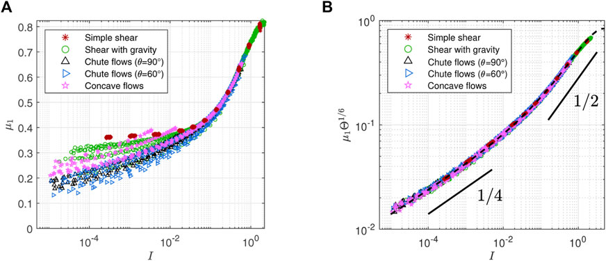
FIGURE 4. (A) Shear stress to pressure ratio μ₁ = |σ_xz|/P vs. inertial number I. Scattered data indicate μ₁ is not a function of I alone. (B) Rescaling μ₁ by the dimensionless temperature to the power of 1/6 makes scattered points collapse into a master curve: μ₁Θ^1/6 = f₁(I). Dashed trend line is f₁(I) used for the FDM simulations in Section 3.

2.3.3 μ₂ measurement

The coefficient of the ${\mathit{D}}^2-\frac{\mathrm{t}\mathrm{r}({\mathit{D}}^2)}{3}\mathit{I}$ term, μ₂, can be calculated as −((σ_xx + σ_zz)/2 − σ_yy)/P according to Eq. 15. It represents a measure of the difference between the normal stress in the vorticity direction and the mean of the other normal stresses. Simply put, the larger the μ₂, the smaller |σ_yy| is compared to the other normal stresses; Figure 5A shows that μ₂ monotonically increases as I increases. This monotonic increase in the μ₂ vs. I graph has also been observed by [45]. As I decreases below 10^–2, similar to μ₁, the data points of μ₂ in inhomogeneous flows become more scattered. The random error in μ₂ measurement seems much larger than μ₁ possibly because μ₂ is measured from the small difference between (σ_xx + σ_zz)/2 and σ_yy accumulating the errors of the three stress elements. Although the μ₂ data are not as clean as μ₁, we can still see that μ₂ exhibits Θ dependence similar to μ₁ where higher Θ lowers μ₂ for a given I. This may imply that μ₂ can also be scaled by a power function of Θ like μ₁. Indeed, multiplying μ₂ by ${\mathrm{\Theta }}^{p_2}$ seems to cancel the non-local spread and collapse the data more onto a single curve when p₂ ≈ 1/6 as shown in Figure 5B:

${\mu }_2{\mathrm{\Theta }}^{p_2}=f_2\left(I\right)(17)$

where f₂(I) can be fitted by $I^{{\alpha }_2}$ where α₂ gradually increases from 0.3 to 0.7 as I increases from 10^–3 to 1. For a fixed I, f₂(I) would increase with μ_p; [45] has similarly shown for homogeneous flows that μ₂ increases with μ_p. For the FDM simulations in Section 3, we use p₂ = 1/6 and f₂(I) = 0.093I^0.29 + 0.195I^1.2 − 0.035I² (dashed line in Figure 5B) which is arbitrarily chosen to represent the collapsed data of the μ_p = 0.4 case.

FIGURE 5

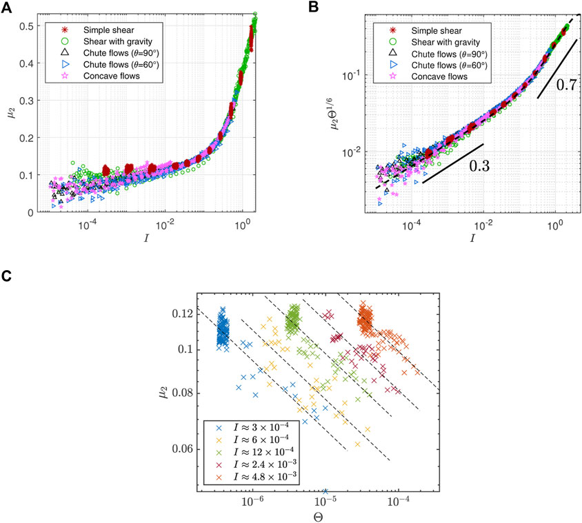
FIGURE 5. (A) μ₂ vs. I in DEM simulations of planar shear flows. Scattered data indicate μ₂ is not a function of I alone. (B) Rescaling μ₂ by ${\mathrm{\Theta }}^{p_2}$ seems to collapse data into a master curve when p₂ ≈ 1/6: μ₂Θ^1/6 = f₂(I). Dashed trend line is f₂(I) used for the FDM simulations in Section 3. (C) Using multivariate linear regression for five selected panels of I, the exponent of μ₂ is measured as 0.154 ± 0.014 (the slope magnitude of dashed lines) for 3D spheres with μ_p = 0.4. Since this error is from the selected data set, the actual error could be larger.

As in [25], we plot μ₂ vs. Θ at many fixed choices of I to see the functional dependence more clearly. We choose five panels of data in 0.9I* < I < 1.1I* for I* = {3 × 10^–4, 6 × 10^–4, 1.2 × 10^–3, 2.4 × 10^–3, 4.8 × 10^–3}. The dashed lines in Figure 5C illustrate the best-fit lines of a multivariate linear regression whose slope is measured as −0.154 ± 0.014 which equals −p₂. The actual error could be larger than this standard error measured only from the chosen data. Since p₂ seems not so different from 1/6 which is the exponent of μ₁ and the data collapse is strong with 1/6 in Figure 5B, we assume both μ₁ and μ₂ scale with the same 1/6 power of Θ for the continuum simulations in Section 3. It remains for further research to identify the exponents and the master curves more accurately.

2.3.4 μ₃ measurement

The coefficient of the DW − WD term, μ₃, can be calculated as (σ_xx − σ_zz)/(4P) according to Eq. 15. It represents a measure of the difference between the normal stresses in the flow direction and the velocity gradient direction; Figure 6A shows that μ₃ is near or slightly above zero for I < 0.1. The only exception is the data from the chute flow geometries, which go up to 0.02. This behavior is significantly different from the non-local effect of granular temperature observed in Figure 4A because the data from the other inhomogeneous flows (the shear with gravity and the concave flows) follow the same curve as the homogeneous flow data, which means flows with different Θ can have the same μ₃ for a given I. Θ is not enough to explain this deviation and there must be other factors that affect the μ₃ measurement in the chute flows. We discuss another possible μ₃ calibration to resolve this issue in the next section. Here, we choose to exclude the problematic chute flow data in calibrating μ₃. Figure 6B shows that, as I increases, μ₃ becomes negative and decreases almost linearly:

${\mu }_3=f_3\left(I\right)(18)$

where f₃(I) ≈ − 0.045I (dashed line) for μ_p = 0.4. For a fixed I, f₃(I) would decrease (increase in magnitude) with μ_p as [45] has shown for homogeneous flows.

FIGURE 6

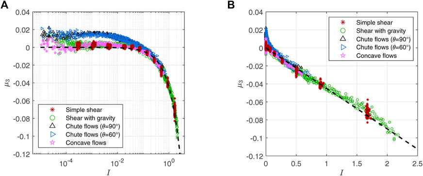
FIGURE 6. (A) μ₃ = (σ_xx − σ_zz)/(4P) vs. I plot using a logarithmic scale on the I-axis. μ₃ is near zero for I < 0.1 except for chute flow data which go up to 0.02. (B) As I increases, μ₃ becomes negative and decreases almost linearly. Dashed trend lines in both plots indicate f₃(I) = −0.045I.

2.3.5 Alternative μ₃ calibration using temperature anisotropy

The chute flows’ peculiar μ₃ behavior in Figure 6A may be attributed to the anisotropy of the granular temperature. This possibility suggests an alternative way to calibrate μ₃ which could be implemented in future work. Let us denote the dimensionless granular temperature tensor as

${\mathrm{\Theta }}_{ij}=\frac{{\rho }_s{T}_{ij}}{P}.(19)$

where T_ij is the (i, j)th element of the granular temperature tensor introduced in Eq. 8. The difference between normal elements in the flow direction and the vorticity direction, Θ_xx − Θ_yy, behaves similarly to μ₃ in that the chute flow data diverge from the other data as I decreases as shown in Figure 7A. The anisotropy of the granular temperature tensor may cause the peculiar behavior of μ₃, or there is another unknown macroscopic variable that affects both Θ_xx − Θ_yy and μ₃ in a similar pattern. In any case, we can calibrate μ₃ using this correlation. For example, adding an arbitrary function $0.4{({\mathrm{\Theta }}_{xx}-{\mathrm{\Theta }}_{yy})}^{1/6}$ to −μ₃ seems to collapse the data more:

$-{\mu }_3+0.4{\left({\mathrm{\Theta }}_{xx}-{\mathrm{\Theta }}_{yy}\right)}^{1/6}\approx f_{3A}\left(I\right)(20)$

as shown in Figure 7B. This collapse only shows the correlation between μ₃ and Θ_xx − Θ_yy in our DEM data. The actual (more accurate) expression for μ₃ may differ from Eq. 20. More diverse Θ_xx − Θ_yy vs. I curves are needed to clearly verify the data collapse as our current flow geometries have generated only two different branches as can be seen in Figure 7A. Also, it is not obvious how to define Θ_xx and Θ_yy in a general flow. Therefore, we leave this problem for future research and choose to use the simpler μ₃ expression, Eq. 18, for the continuum simulations in Section 3.

FIGURE 7

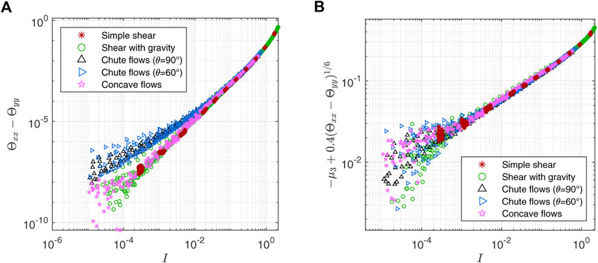
FIGURE 7. (A) Difference between two diagonal elements of dimensionless granular temperature tensor (Θ_xx − Θ_yy). Chute flow data diverge from the other data as I decreases, which is similar to the μ₃ behavior in Figure 6A. (B) Adding $0.4{({\mathrm{\Theta }}_{xx}-{\mathrm{\Theta }}_{yy})}^{1/6}$ to −μ₃ may be an alternative way to calibrate μ₃ because it seems to collapse data into a line.

2.3.6 Normal stress differences

In this section, we examine the first and second normal stress differences as they are commonly measured quantities to represent the normal stress anisotropy of a material, even though we do not utilize them explicitly in our continuum model. The first normal stress difference is defined as N₁ = σ_xx − σ_zz which is the same as 4μ₃P (Eq. 15). Figure 8A shows that N₁/P is almost zero for I < 10^–1 and grows negative as I increases above 10^–1. It means that, as I increases, the magnitude of stress in the flow direction |σ_xx| becomes larger than that in the gradient direction |σ_zz|. This is consistent with previous observations in 2D and 3D granular systems [35, 36, 38–40, 43, 45]. The peculiar chute data do not collapse into a single line even if the horizontal axis is changed to |σ_xz/σ_zz| as can be seen in Figure 8B.

FIGURE 8

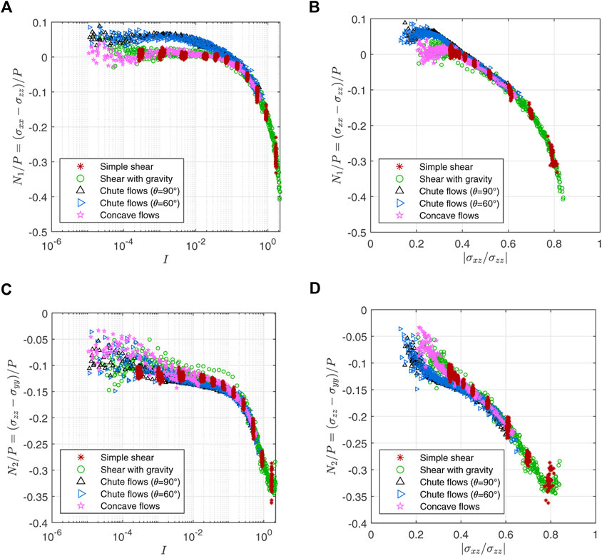
FIGURE 8. Variation of the first (N₁) and second (N₂) normal stress differences divided by pressure: The first row is N₁/P = (σ_xx − σ_zz)/P plotted against (A) I and (B) |σ_xz/σ_zz|. N₁/P is close to zero for I < 10^–1 and grows negative as I increases above 10^–1. The second row is N₂/P = (σ_zz − σ_yy)/P plotted against (C) I and (D) |σ_xz/σ_zz|. N₂ is always negative for a non-zero I

On the other hand, the second normal stress difference N₂ = σ_zz − σ_yy represents normal stress anisotropy in the plane formed by the velocity gradient and the vorticity directions. N₂ can be written as −(μ₂ + 2μ₃)P (Eq. 15). Figure 8C displays that N₂/P behaves like μ₁ and μ₂ in that the inhomogeneous flow data are scattered and the simple shear data do not converge to zero in the quasi-static regime. However, the chute flow data are still a bit out of the trend. This peculiarity is more noticeable when the horizontal axis is |σ_xz/σ_zz| as shown in Figure 8D. All the other N₂/P data seem to form a single line while the chute data with |σ_xz/σ_zz| < 0.4 have lower N₂/P values. Another important feature of Figure 8C is that N₂ is always negative for a non-zero I, which is in line with previous observations [37, 43, 45]. It has been known that a negative N₂ makes the free surface convex up in a channel flow with no surface tension [29, 54–57]. This convex surface is also observed in our inclined chute flow simulations in Section 3.

If we look closely at Figures 8B, D where the horizontal axes are |σ_xz/σ_zz|, the chute flow data go higher than the other data in Figure 8B and lower in Figure 8D. Because the peculiar chute deviations have opposite signs in N₁ and N₂, we are intrigued to observe their sum N₁ + N₂. This variable is actually another normal stress difference σ_xx − σ_yy. Interestingly, (N₁ + N₂)/P exhibits a collapsed line when the horizontal axis is |σ_xz/σ_zz| canceling the above deviations as displayed in Figure 9B. Meanwhile; Figure 9A demonstrates that (N₁ + N₂)/P vs. I plot does not form a collapsed line and its pattern is similar to vertically flipped μ₁ vs. I plot (Figure 4A). Therefore, (N₁ + N₂)/P may depend only on |σ_xz/σ_zz| or μ₁.

FIGURE 9

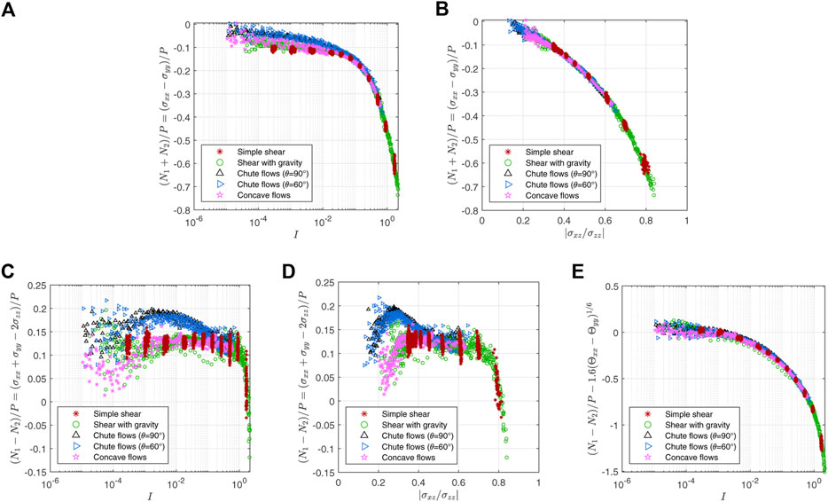
FIGURE 9. Sum and difference of the first (N₁) and second (N₂) normal stress differences divided by pressure: (N₁ + N₂)/P = (σ_xx − σ_yy)/P exhibits non-locality when plotted against I (A), but it forms a collapsed line when plotted against |σ_xz/σ_zz| (B). Plotting (N₁ − N₂)/P = (σ_xx + σ_yy −2σ_zz)/P against (C) I or (D) |σ_xz/σ_zz| does not form a data collapse. (E) Subtracting an arbitrary function $1.6{({\mathrm{\Theta }}_{xx}-{\mathrm{\Theta }}_{yy})}^{1/6}$ from (N₁ − N₂)/P seems to collapse the data into a line that depends only on I.

If (N₁ + N₂)/P is indeed a function of |σ_xz/σ_zz| or μ₁, we need one more equation to represent N₁ and N₂ separately. (N₁ − N₂)/P may provide that equation. However, Figures 9C, D show that (N₁ − N₂)/P plots whose horizontal axis is I or |σ_xz/σ_zz| do not have a well-collected collapse in contrast to the collapse seen in Figure 9B. (N₁ − N₂)/P is almost a constant between 0.1 and 0.15 except for the chute data which go up to 0.2. It seems as if the peculiarity of the chute data is canceled in the (N₁ + N₂)/P plot and pushed into the (N₁ − N₂)/P plot to become more conspicuous. Although (N₁ − N₂)/P cannot be written as a function of a single dimensionless variable, we can still utilize Θ_xx − Θ_yy in Figure 7A. For example, Figure 9E demonstrates that subtracting $1.6{({\mathrm{\Theta }}_{xx}-{\mathrm{\Theta }}_{yy})}^{1/6}$ from (N₁ − N₂)/P reduces the chute data peculiarity and collapses the data into a curve that depends only on I.

Using (N₁ + N₂)/P and (N₁ − N₂)/P data collapses, we may solve for μ₂ and μ₃ in terms of I, Θ and Θ_xx − Θ_yy. However, as mentioned above, Θ_xx − Θ_yy in a more complex flow geometry is not simple to define. Also, the data collapse in 9E is not yet clear because it is achieved only for two big branches of (N₁ − N₂)/P while adding an arbitrary function with two fitting parameters. Thus, further research is needed to build a more general rheological model that incorporates the temperature anisotropy and its impact on (N₁ − N₂)/P.

3 Model validation: Inclined chute flows

In this section, we show how our second-order non-local model can be applied to a more complex flow geometry with less symmetry. For that, we use data from DEM simulations of rough-walled inclined chute flows (Figure 10A) gathered in [25]. Unlike the planar shear flows used in calibration where the time-averaged macroscopic quantities depend only on the height (z), in this inclined chute geometry, the mean fields depend on two spatial coordinates (y and z). Moreover, the mean velocity fields have three non-zero components forming a secondary flow. The expression for stress becomes more complicated than Eq. 14 because the velocity gradient tensor now has six non-zero terms (the derivatives with respect to the downstream coordinate (x) are still negligible due to symmetry). We demonstrate that our model calibrated from the simple tests can be applied to this complex case. We run finite difference method (FDM) simulations of the full partial differential equation (PDE) system of the model, including Eq. 5 and continuum momentum balance to compare with DEM results. Unlike [25], the current model is able to describe the transverse secondary flow which is perpendicular to the downstream direction and could not be predicted by the first-order model.

FIGURE 10

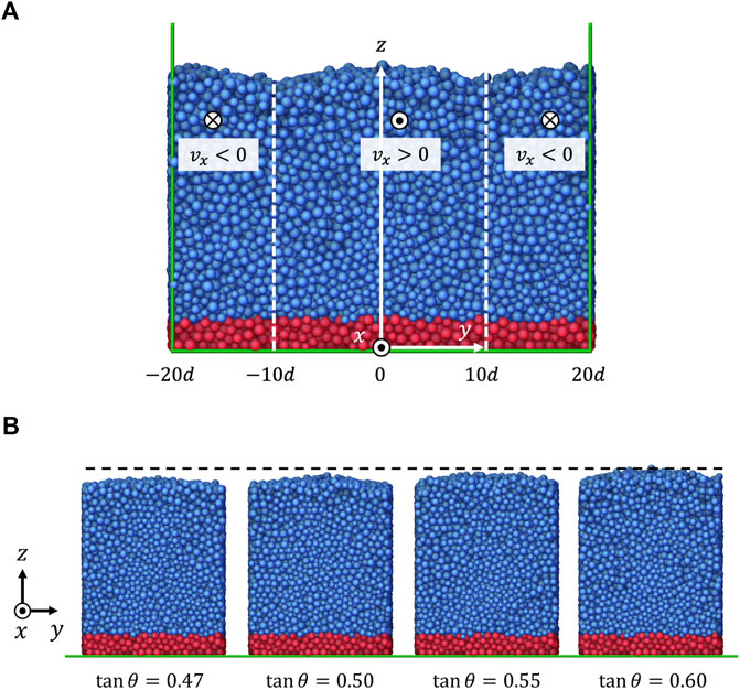
FIGURE 10. (A) DEM simulation of inclined chute flow with θ = tan⁻¹(0.60). Green lines are boundaries of the DEM simulation domain which is periodic in x and y directions. v_x is positive in the middle zone (−10d < y <10d) where gravity is $\vec{G}=G\sin \theta \widehat{x}+G\cos \theta \widehat{z}$ and negative in the rest where gravity is $\vec{G}=-G\sin \theta \widehat{x}+G\cos \theta \widehat{z}$. Red particles are fixed. (B) Inclined chute flows with different inclination angles viewed from the positive x-axis. Only particles in −10d < y < 10d are shown. Dashed line indicates the maximum height of the surface for tanθ = 0.60. From the gaps between the dashed line and the surfaces, we can see that the volume of the material increases as the inclination angle increases and the material flows faster. The surface becomes convex due to normal stress anisotropy.

3.1 DEM simulation settings for inclined chute flows

Using the same granular material used in the planar shear tests, we run the inclined chute flow simulations for four inclination angles: θ = tan⁻¹(0.47), tan⁻¹(0.50), tan⁻¹(0.55), and tan⁻¹(0.60). Figure 10A shows a snapshot of the θ = tan⁻¹(0.60) case. The size of the system is L_x = 120d, L_y = 40d. The simulation domain (green lines) is periodic in the x and y-directions. A total of 131,566 particles are simulated. For a rough frictional bottom, the particles whose center height is lower than z = 3d (colored red in Figure 10A) are frozen; their translational and rotational velocities are fixed to zero. Except for these fixed particles, there are 115,619 mobile particles (colored blue in Figure 10A). Gravity is applied differently in the middle zone (−10d < y < 10d) and the outer zone (y < − 10d or y > 10d). In the middle zone, gravity is tilted in the x-direction $(\vec{G}=G\sin \theta \widehat{x}-G\cos \theta \widehat{z})$ and, in the outer zone, gravity is tilted in the −x-direction $(\vec{G}=-G\sin \theta \widehat{x}-G\cos \theta \widehat{z})$. If we denote the time-averaged velocity field as $\vec{v}=(v_x,v_y,v_z)$, this setting naturally sets v_x and v_y to be zero at the effective side boundaries (y = −10d and 10d) but without unwanted wall effects. v_z should be continuous across the side boundaries but does not need to be zero. More detailed simulation conditions are in Supplementary Material.

At steady state, we measure the continuum fields $\vec{v}$, T, σ, ϕ, and $\bar{d}$ (average particle diameter) using Eqs 6–9 at 97 × 97 grid points (y_k = [−12, − 11.75, … , 11.75, 12]d and z_k = [3, 3.25, … , 26.75, 27]d). The weight of averaging here is chosen to be the overlap length (not area) between the line of (y_k, z_k) and each particle. $\bar{d}$ is obtained in the same way as $\vec{v}$. All the continuum variables at each (y_k, z_k) are then averaged over time.

Figure 10B illustrates snapshots of the simulations with different inclination angles viewed from the positive x-axis. It shows that the maximum height of the material increases as the inclination angle increases. This volume increase can be explained by the ϕ(μ) relation found in [25], which claims that the volume density decreases as μ increases at steady state. As discussed previously, it is also observed that the shape of the top surface is convex such that the grains in the middle of the surface keep falling to the side boundaries where the surface is lower. This convex surface is formed possibly because the second normal stress difference N₂ is negative.

3.2 Continuum simulation methods

In this section, stress and velocity fields in inclined chute flows are predicted by the second-order non-local model using an explicit FDM scheme. We compute the stress field σ using Eq. 5 combined with Eqs. 16-18.

To predict the flow, we numerically solve the Cauchy momentum equation given by

$\rho \frac{\partial \mathit{v}}{\partial t}+\rho \left(\mathit{v}\cdot \nabla \right)\mathit{v}=\nabla \cdot \mathit{\sigma }+\rho \mathit{G}(21)$

where $\mathit{v}=v_x\widehat{\mathit{x}}+v_y\widehat{\mathit{y}}+v_z\widehat{\mathit{z}}$ is the velocity field, ρ = ρ_sϕ is the mass density, and $\mathit{G}=G\sin \theta \widehat{\mathit{x}}-G\cos \theta \widehat{\mathit{z}}$ is gravity. Instead of adding a continuity equation of mass conservation, we input the density data from the DEM simulations. The physical domain is chosen from y = 0 to y = 10d in the y-direction and from z_min = 5.49d to z_max = 24.25d in the z-direction where z_min is 2d above the average z values of the lowest particles and z_max is the highest grid point with ϕ > 0.2 along the line of y = 10d. The material is also present above z = z_max forming the convex surface. Ghost nodes around the physical domain are added to set the pressure and velocity fields to satisfy the boundary conditions. Since z = z_max does not exactly match the material surface, we input the traction $\mathit{\sigma }\cdot \widehat{\mathit{z}}$ extracted from the DEM simulations as the upper boundary condition. By the symmetry of the geometry, v_y = 0 at y = 0, and v_x = 0 and v_y = 0 at y = 10d. The velocity at z = z_min is set to be zero. A schematic diagram of the FDM simulation grid is illustrated in Supplementary Material.

We use the projection method which is an efficient algorithm for solving the time-dependent Navier-Stokes equations in incompressible flows [58]. It needs to be modified a little from Chorin’s original projection method because our fluid is not incompressible. This algorithm allows us to calculate the pressure field easily by decoupling the pressure and the velocity fields. We decompose the stress into σ′ = σ + PI and −PI which results in two differential equations connected by an intermediate velocity v*. The first step of the projection method algorithm is to update v* from the current velocity vⁿ through

${\mathit{v}}^{*}={\mathit{v}}^n+\mathrm{\Delta }t\left[-\left({\mathit{v}}^n\cdot \nabla \right){\mathit{v}}^n+\frac{1}{\rho }\nabla \cdot {\mathit{\sigma }}^{\prime }+\mathit{G}\right](22)$

where Δt is the FDM time step. The next step of the algorithm is to correct v* to obtain the velocity in the next step vⁿ⁺¹:

${\mathit{v}}^{n+1}={\mathit{v}}^{*}-\frac{\mathrm{\Delta }t}{\rho }\nabla P^{n+1}(23)$

where the pressure in the next step Pⁿ⁺¹ can be obtained by solving a Poisson-type equation. We multiply Eq. 23 by ρ and take the divergence. We assume ∇ ⋅ (ρvⁿ⁺¹) = 0 because we are interested in steady state where the (Eulerian-frame) density field does not change in time $(\frac{\partial \rho }{\partial t}=0)$. Keeping the spatial variations in density, the pressure field should thus satisfy

${\nabla }^2{P}^{n+1}=\frac{1}{\mathrm{\Delta }t}\nabla \cdot \left(\rho {\mathit{v}}^{*}\right).(24)$

The pressure should be symmetrically distributed across the side boundaries due to the specificity of the geometry. The bottom pressure should satisfy $\frac{\partial P}{\partial z}=\frac{\rho }{\mathrm{\Delta }t}{v}_z^{*}$ from Eq. 23 to ensure $\vec{v}=0$ at z = z_min. In DEM, there is actually a tiny non-zero velocity at z = z_min because z_min is slightly (2d) above the fixed bottom particles, but we neglect this small velocity in our FDM simulations. The pressure at the upper boundary is calculated from DEM σ_zz data and the extrapolated velocity gradient there. Details of the numerical method to solve Eq. 24 are in Supplementary Material.

Using MATLAB, we numerically solve the decomposed momentum equations, Eqs 22, 23, on a 20 × 40 stress grid. We use the local density measured in the DEM simulations. Since we do not know how to predict Θ, we simply insert the DEM data of Θ into μ₁(I, Θ) and μ₂(I, Θ) calibrated as Eqs 16, 17 respectively to obtain the stress tensor defined in Eq. 5. The granular temperature should follow a separate PDE, “fluctuation energy balance” in the kinetic theory [21, 22, 59], but its form is still under debate in the dense limit. To predict Θ, this PDE should be clarified in the future. The general form of the fluctuation energy balance is in Supplementary Material. We use Eq. 18 for μ₃(I). Pressure is obtained from the Poisson equation, Eq. 24. We input the traction force extracted from the DEM data at the top of the FDM domain because our FDM grid is rectangular and does not conform to the bulged shape of the free surface. The velocity is updated until the system’s average velocity reaches a steady state.

3.3 Analysis of model predictions

We compare the results of the DEM simulations and the continuum simulations varying the inclination angle from θ = tan⁻¹(0.47) to tan⁻¹(0.60). Figure 11 illustrates the transverse velocity fields (v_y, v_z) from the DEM data (upper row) and the FDM solutions to the second-order model (lower row). The predicted transverse velocity fields show remarkable similarity to the DEM velocity data especially for the faster flows with larger inclination angles. We can see that the vortex location (center of the rotational flow) and the magnitude of transverse velocity (length of the arrows) are successfully predicted. The second-order model’s ability to predict these transverse flows is a huge improvement from the first-order model.

FIGURE 11

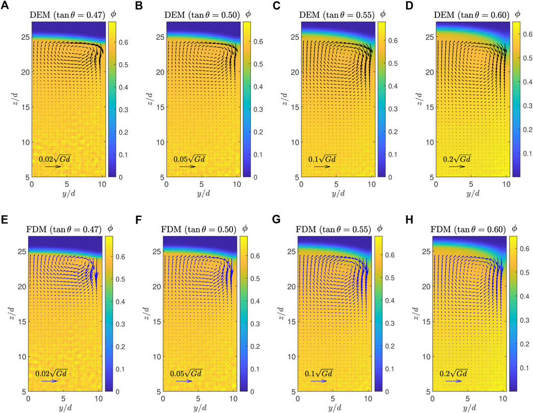
FIGURE 11. Transverse velocity comparison between the DEM simulations (A–D) and the FDM simulations using the second-order model (E–H): (A) DEM with tan θ = 0.47, (E) FDM with tan θ = 0.47, (B) DEM with tan θ = 0.50, (F) FDM with tan θ = 0.50, (C) DEM with tan θ = 0.55, (G) FDM with tan θ = 0.55, (D) DEM with tan θ = 0.60, and (H) FDM with tan θ = 0.60. Arrows indicate (v_y, v_z) and their length scales are displayed at the bottom of the figures. Packing fraction is shown as color in the background.

This predictive power mostly comes from μ₂ in our geometry. μ₃ has a relatively smaller impact on the results. If we keep μ₃ and set μ₂ to zero, the prediction becomes totally different from DEM. However, if we keep μ₂ and set μ₃ to zero, the FDM simulation still generates similar secondary flows even though the results are not as accurate as the full second-order model’s. These results are shown in Supplementary Material.

The solution of the first-order model must have zero transverse velocities for a free surface flow (no surface traction). Without μ₂ and μ₃, v = (v_x(y, z), 0, 0) can satisfy the momentum balance (Eq. 21), which is discussed in Supplementary Material. If an external traction is applied, the first-order model can have non-zero v_y and v_z. In this case, σ_yz is no longer zero and transverse velocities are generated to match this stress. However, we have checked that the first-order models’ FDM solutions to the transverse velocities are completely different from the DEM data. The results can be found in Supplementary Material.

Figure 11E indicates that the transverse velocity prediction slightly mismatches the DEM data for tan θ = 0.47. That is, possibly because the transverse velocity is too small compared to the error of the model calibration, or the highest grid points are too close to the material surface where the packing fraction drops rapidly and the granular temperature anisotropy is strong. We could not lower the highest grid points as the vortex location is about 2d below the surface for tan θ = 0.47. This issue may be resolved by a more accurate modeling including the whole granular temperature tensor and a deformable grid to effectively exclude areas where ϕ drops rapidly.

The downstream velocity v_x is accurately predicted by our model as the first-order non-local model did in [25]. This is expected because the shear stress associated with D is determined by a function μ₁(I, Θ) which is almost identical to the previous μ(I, Θ) while the other higher-order terms have little impact on v_x. Figures 12A–D illustrates the contours of $v_x/\sqrt{Gd}$ from the DEM simulations and the FDM simulations using the second-order model for four different inclination angles. The magnitude of velocity varies greatly from $10^{-4}\sqrt{Gd}$ to $2.5\sqrt{Gd}$, but the FDM v_x contours almost exactly match the DEM v_x contours for all the inclination angles. The inertial number contours are also well predicted from the quasi-static to inertial regimes as displayed in Figures 12E–H. The excellent agreement between the FDM solutions and the DEM data in Figures 12I, J clearly demonstrates that the second-order model can successfully capture the exponentially decaying v_x and I profiles at the chute’s center plane (y = 0). The minor mismatches near the bottom (z < 8d) in Figure 12 are due to the fact that DEM v_x is not exactly zero at the lower boundary while we set it to zero in the FDM simulations. This issue can be resolved if the slip condition at the solid boundary is clarified.

FIGURE 12

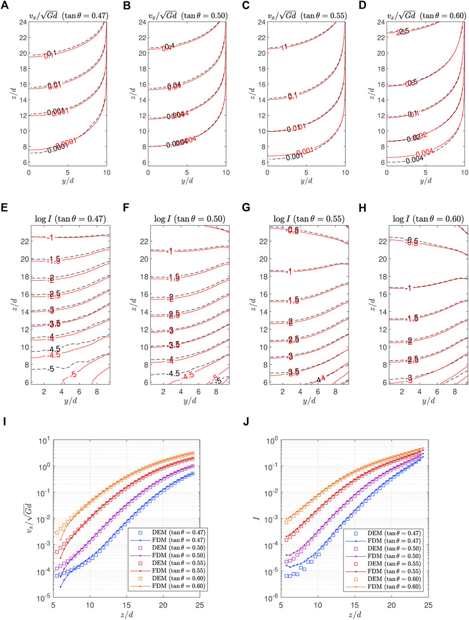
FIGURE 12. Comparison of (A–D) $v_x/\sqrt{Gd}$ and (E–H) log  I contours between the DEM simulations (black dashed lines) and the FDM simulations using the second-order model (red lines) for different inclination angles: (A, E) tan θ = 0.47, (B, F) tan θ = 0.50, (C, G) tan θ = 0.55, and (D, H) tan θ = 0.60. (I) $v_x/\sqrt{Gd}$ and (J) I profiles of the DEM simulations (squares) and the FDM predictions (lines) at the center plane (y = 0).

The second-order model’s pressure P is obtained by solving the Poisson equation, Eq. 24, with the boundary conditions described in Section 3.2. Figure 13A visualizes the results for tan θ = 0.60. If the granular material is static and its density is uniform, the pressure increases linearly in proportion to the depth H − z where H is the surface height. However, the pressure in the inclined chute flow slightly deviates from this lithostatic pressure because the surface becomes not flat due to the normal stress anisotropy. To make this subtle deviation stand out, we subtract a linear function $\bar{\rho }{G}_z(H-z)$ from the pressure results. We choose H = 25.4d and $\bar{\rho }=0.538{\rho }_s$ to best fit the DEM |σ_yy| which has the most linear profile among the normal stresses. The DEM pressure is lower near the top-right corner and this gradation is accurately predicted by the second-order model as can be seen in the similarity between the two heat maps in Figure 13A. The prediction error is insignificant compared to the magnitude of pressure. The pressure difference between DEM and FDM is up to 40 Pa which is only 4% of the bottom pressure of 1.1 Pa × 10³ Pa.

FIGURE 13

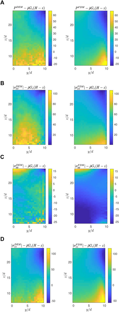
FIGURE 13. Comparison of pressure and normal stress maps between the DEM simulation (left) and the FDM simulation using the second-order model (right) with tan θ = 0.60: (A) $P-\bar{\rho }{G}_z(H-z)$, (B) $|{\sigma }_{xx}|-\bar{\rho }{G}_z(H-z)$, (C) $|{\sigma }_{yy}|-\bar{\rho }{G}_z(H-z)$, and (D) $|{\sigma }_{zz}|-\bar{\rho }{G}_z(H-z)$ where $\bar{\rho }{G}_z(H-z)$ is a reference pressure linearly decreasing from 1.1 Pa × 10³ Pa at z = 24.5d to 54 Pa at z = 7d.

From the pressure, the granular temperature, and the velocity field, the stress tensor is computed through Eq. 5. Overall, the predictions of the second-order model on stress are well matched with the DEM results. Figure 13 illustrates the differences between the normal stresses and the linear reference pressure for tan θ = 0.60. The second-order model successfully predicts the large deviations of σ_xx and σ_zz from the linear reference pressure as shown in Figures 13B, D. Figure 13C demonstrates that σ_yy is flatter than the other components, which is also well captured by the FDM simulation. The patterns of σ_yy seem different in Figure 13C, but the actual error is insignificant considering that the colorbar range is narrower than the other plots.

The off-diagonal elements of the stress tensor are also well predicted by the second-order model. Figure 14 shows that the model predicts the gradual variations of σ_xy/P, σ_xz/P, and σ_yz/P accurately in the inclined chute flow with tan θ = 0.60. In particular, it is interesting to see the model’s ability to estimate σ_yz in Figure 14C while having accurate velocity fields because this component is much smaller than the other stresses and predicted to be zero in the first-order model. The first-order model may produce similar σ_xy, σ_xz and pressure patterns. However, it cannot predict the normal stress differences and σ_yz because it predicts zero transverse velocities and a flat surface, which results in an isotropic pressure and zero σ_yz.

FIGURE 14

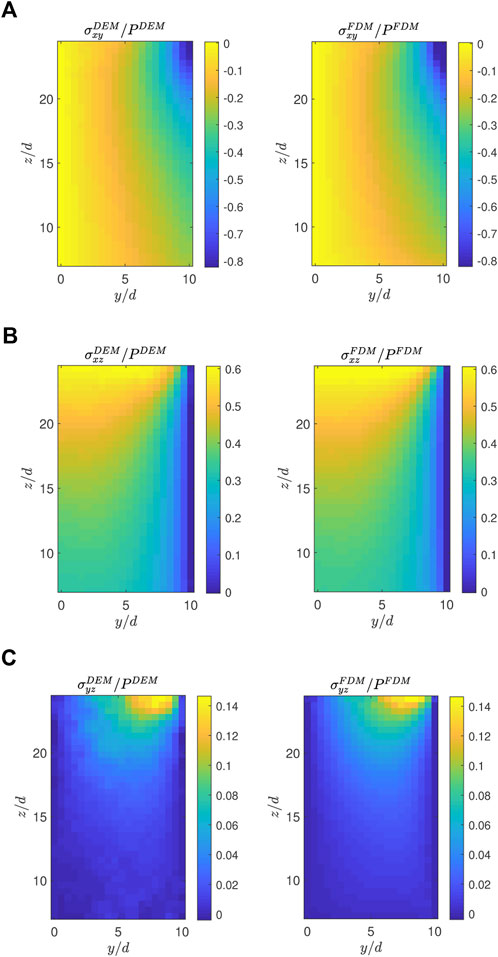
FIGURE 14. Comparison of off-diagonal stress maps between the DEM simulation (left) and the FDM simulation using the second-order model (right) with tan θ =0.60: (A) σ_xy/P, (B) σ_xz/P, and (C) σ_yz/P.

4 Conclusion

Combining the μ(I, Θ) model and the second-order fluid model, we have proposed a second-order temperature-dependent model for three-dimensional granular flows that can describe both non-local phenomena (arising from the diffusion implicit in the temperature field) and broken codirectionality. From DEM data of planar shear tests, we have identified the model parameters μ₁, μ₂, and μ₃ as functions of I and Θ. As in the μ(I, Θ) model, μ₁ multiplied by ${\mathrm{\Theta }}^{p_1}$ collapses into a sole function of I where p₁ ≈ 1/6. μ₂ is always positive even for small I and exhibits heat-softening effects; μ₂ seems to be scaled by a power function of Θ with an exponent not far from p₁ even if its data collapse is inherently noisier. Excluding anomalous chute flow data, μ₃ appears to be a monotonically decreasing function of I alone, which is almost zero for small I and grows negative as I increases. We have observed that Θ_xx − Θ_yy behaves similar to μ₃, implying that μ₃ may be affected by the granular temperature anisotropy, causing the observed anomaly.

In addition, we have examined the first and second normal stress differences N₁ and N₂ in the same geometry. N₂/P is negative and decreases as I increases, exhibiting Θ dependence similar to μ₁ and μ₂. By adding N₁/P and N₂/P together, a clear data collapse has been achieved forming a function of the shear-to-normal stress ratio. We have also seen the possibility that (N₁ − N₂)/P is a function of I and Θ_xx − Θ_yy, but more rigorous verification is needed in the future.

Using the model parameters calibrated from the planar shear flows, we have validated the second-order model in the rough-walled inclined chute geometry, which is more complex due to less symmetry. We have run FDM simulations using the projection method inputting DEM traction at the upper boundary and DEM Θ for the whole domain. Our second-order model successfully describes the the flow field including the transverse secondary flows which the first-order models fail to capture. The location, size, and shape of the flow vortex in the secondary flow is well matched by the FDM simulations including how the vortex changes with the inclination angle. We have also found that μ₂ plays a more important role than μ₃ in predicting the transverse velocities even if μ₂ and μ₃ together have better predictions. The second-order model, like the μ(I, Θ) model, has also accurately predicted the downstream velocity fields including the quasi-static creeping regime. Moreover, the second-order model has generated almost identical pressure and normal stress patterns as the DEM data.

Although we have made significant progress towards more accurate granular rheology by combining the μ(I, Θ) relation and a second-order fluid model to describe non-locality and broken codirectionality, there are still puzzles to be solved. For example, the governing equation of the granular temperature should be precisely identified to complete the model. While the current model utilizes a scalar temperature, the aforementioned potential role of temperature tensor anisotropy suggests a tensorial heat equation may be needed to go beyond the accuracy level of the model shown herein. Also, the constitutive relation could be further intertwined with the granular temperature tensor and the strain rate tensor. Solving these problems will refine our model, enabling even more accurate and universal prediction of granular flows.

Data availability statement

The raw data supporting the conclusion of this article will be made available by the authors, without undue reservation.

Author contributions

SK and KK contributed to the conception of the study and the design of tests. SK performed all numerical simulations, conducted the data analysis, and wrote the first draft. KK contributed to draft revisions. SK and KK approved the submitted work.

Funding

SK and KK acknowledge funding from Army Research Office grant W911NF-19-1-0431.

Conflict of interest

The authors declare that the research was conducted in the absence of any commercial or financial relationships that could be construed as a potential conflict of interest.

Publisher’s note

All claims expressed in this article are solely those of the authors and do not necessarily represent those of their affiliated organizations, or those of the publisher, the editors and the reviewers. Any product that may be evaluated in this article, or claim that may be made by its manufacturer, is not guaranteed or endorsed by the publisher.

Supplementary material

The Supplementary Material for this article can be found online at: https://www.frontiersin.org/articles/10.3389/fphy.2023.1092233/full#supplementary-material

References

1.GDR MiDi. On dense granular flows. The Eur Phys J E (2004) 14:341–65. doi:10.1140/epje/i2003-10153-0

PubMed Abstract | CrossRef Full Text | Google Scholar

2. da Cruz F, Emam S, Prochnow M, Roux JN, Chevoir F. Rheophysics of dense granular materials: discrete simulation of plane shear flows. Phys Rev E (2005) 72:021309. doi:10.1103/PhysRevE.72.021309

CrossRef Full Text | Google Scholar

3. Jop P, Forterre Y, Pouliquen O. A constitutive law for dense granular flows. Nature (2006) 441:727–30. doi:10.1038/nature04801

PubMed Abstract | CrossRef Full Text | Google Scholar

4. Jop P, Forterre Y, Pouliquen O. Initiation of granular surface flows in a narrow channel. Phys Fluids (2007) 19:088102. doi:10.1063/1.2753111

CrossRef Full Text | Google Scholar

5. Koval G, Roux JN, Corfdir A, Chevoir F. Annular shear of cohesionless granular materials: from the inertial to quasistatic regime. Phys Rev E (2009) 79:021306. doi:10.1103/PhysRevE.79.021306

PubMed Abstract | CrossRef Full Text | Google Scholar

6. Komatsu TS, Inagaki S, Nakagawa N, Nasuno S. Creep motion in a granular pile exhibiting steady surface flow. Phys Rev Lett (2001) 86:1757–60. doi:10.1103/PhysRevLett.86.1757

PubMed Abstract | CrossRef Full Text | Google Scholar

7. Martinez E, Gonzalez-Lezcano A, Batista-Leyva AJ, Altshuler E. Exponential velocity profile of granular flows down a confined heap. Phys Rev E (2016) 93:062906. doi:10.1103/PhysRevE.93.062906

PubMed Abstract | CrossRef Full Text | Google Scholar

8. Tang Z, Brzinski TA, Shearer M, Daniels KE. Nonlocal rheology of dense granular flow in annular shear experiments. Soft Matter (2018) 14:3040–8. doi:10.1039/C8SM00047F

PubMed Abstract | CrossRef Full Text | Google Scholar

9. Falk ML, Langer JS. Dynamics of viscoplastic deformation in amorphous solids. Phys Rev E (1998) 57:7192–205. doi:10.1103/PhysRevE.57.7192

CrossRef Full Text | Google Scholar

10. Lemaître A. Rearrangements and dilatancy for sheared dense materials. Phys Rev Lett (2002) 89:195503. doi:10.1103/PhysRevLett.89.195503

PubMed Abstract | CrossRef Full Text | Google Scholar

11. Lois G, Lemaître A, Carlson JM. Numerical tests of constitutive laws for dense granular flows. Phys Rev E (2005) 72:051303. doi:10.1103/PhysRevE.72.051303

PubMed Abstract | CrossRef Full Text | Google Scholar

12. Aranson IS, Tsimring LS. Continuum description of avalanches in granular media. Phys Rev E (2001) 64:020301. doi:10.1103/PhysRevE.64.020301

PubMed Abstract | CrossRef Full Text | Google Scholar

13. Aranson IS, Tsimring LS. Continuum theory of partially fluidized granular flows. Phys Rev E (2002) 65:061303. doi:10.1103/PhysRevE.65.061303

PubMed Abstract | CrossRef Full Text | Google Scholar

14. Volfson D, Tsimring LS, Aranson IS. Order parameter description of stationary partially fluidized shear granular flows. Phys Rev Lett (2003) 90:254301. doi:10.1103/PhysRevLett.90.254301

PubMed Abstract | CrossRef Full Text | Google Scholar

15. Goyon J, Colin A, Ovarlez G, Ajdari A, Bocquet L. Spatial cooperativity in soft glassy flows. Nature (2008) 454:84–7. doi:10.1038/nature07026

PubMed Abstract | CrossRef Full Text | Google Scholar

16. Bocquet L, Colin A, Ajdari A. Kinetic theory of plastic flow in soft glassy materials. Phys Rev Lett (2009) 103:036001. doi:10.1103/PhysRevLett.103.036001

PubMed Abstract | CrossRef Full Text | Google Scholar

17. Kamrin K, Koval G. Nonlocal constitutive relation for steady granular flow. Phys Rev Lett (2012) 108:178301. doi:10.1103/PhysRevLett.108.178301

PubMed Abstract | CrossRef Full Text | Google Scholar

18. Henann DL, Kamrin K. A predictive, size-dependent continuum model for dense granular flows. Proc Natl Acad Sci U S A (2013) 110:6730–5. doi:10.1073/pnas.1219153110

PubMed Abstract | CrossRef Full Text | Google Scholar

19. Kamrin K, Henann DL. Nonlocal modeling of granular flows down inclines. Soft Matter (2015) 11:179–85. doi:10.1039/c4sm01838a

PubMed Abstract | CrossRef Full Text | Google Scholar

20. Zhang Q, Kamrin K. Microscopic description of the granular fluidity field in nonlocal flow modeling. Phys Rev Lett (2017) 118:058001. doi:10.1103/PhysRevLett.118.058001

PubMed Abstract | CrossRef Full Text | Google Scholar

21. Jenkins JT, Savage SB. A theory for the rapid flow of identical, smooth, nearly elastic, spherical particles. J Fluid Mech (1983) 130:187–202. doi:10.1017/S0022112083001044

CrossRef Full Text | Google Scholar

22. Lun CKK, Savage SB, Jeffrey DJ, Chepurniy N. Kinetic theories for granular flow: inelastic particles in Couette flow and slightly inelastic particles in a general flowfield. J Fluid Mech (1984) 140:223–56. doi:10.1017/S0022112084000586

CrossRef Full Text | Google Scholar

23. Garzó V, Dufty JW. Dense fluid transport for inelastic hard spheres. Phys Rev E (1999) 59:5895–911. doi:10.1103/PhysRevE.59.5895

CrossRef Full Text | Google Scholar

24. Jenkins JT, Berzi D. Dense inclined flows of inelastic spheres: Tests of an extension of kinetic theory. Granular Matter (2010) 12:151–8. doi:10.1007/s10035-010-0169-8

CrossRef Full Text | Google Scholar

25. Kim S, Kamrin K. Power-law scaling in granular rheology across flow geometries. Phys Rev Lett (2020) 125:088002. doi:10.1103/PhysRevLett.125.088002

PubMed Abstract | CrossRef Full Text | Google Scholar

26. Félix G, Thomas N. Relation between dry granular flow regimes and morphology of deposits: formation of levées in pyroclastic deposits. Earth Planet Sci Lett (2004) 221:197–213. doi:10.1016/S0012-821X(04)00111-6

CrossRef Full Text | Google Scholar

27. Deboeuf S, Lajeunesse E, Dauchot O, Andreotti B. Flow rule, self-channelization, and levees in unconfined granular flows. Phys Rev Lett (2006) 97:158303. doi:10.1103/PhysRevLett.97.158303

PubMed Abstract | CrossRef Full Text | Google Scholar

28. Takagi D, McElwaine JN, Huppert HE. Shallow granular flows. Phys Rev E (2011) 83:031306. doi:10.1103/PhysRevE.83.031306

PubMed Abstract | CrossRef Full Text | Google Scholar

29. McElwaine JN, Takagi D, Huppert HE. Surface curvature of steady granular flows. Granular Matter (2012) 14:229–34. doi:10.1007/s10035-012-0339-y

CrossRef Full Text | Google Scholar

30. Gutam KJ, Mehandia V, Nott PR. Rheometry of granular materials in cylindrical Couette cells: Anomalous stress caused by gravity and shear. Phys Fluids (2013) 25:070602. doi:10.1063/1.4812800

CrossRef Full Text | Google Scholar

31. Fischer D, Börzsönyi T, Nasato DS, Pöschel T, Stannarius R. Heaping and secondary flows in sheared granular materials. New J Phys (2016) 18:113006. doi:10.1088/1367-2630/18/11/113006

CrossRef Full Text | Google Scholar

32. Krishnaraj KP, Nott PR. A dilation-driven vortex flow in sheared granular materials explains a rheometric anomaly. Nat Commun (2016) 7:10630. doi:10.1038/ncomms10630

PubMed Abstract | CrossRef Full Text | Google Scholar

33. Dsouza PV, Nott PR. Dilatancy-driven secondary flows in dense granular materials. J Fluid Mech (2021) 914:A36. doi:10.1017/jfm.2020.1029

CrossRef Full Text | Google Scholar

34. Mehandia V, Gutam KJ, Nott PR. Anomalous stress profile in a sheared granular column. Phys Rev Lett (2012) 109:128002. doi:10.1103/PhysRevLett.109.128002

PubMed Abstract | CrossRef Full Text | Google Scholar

35. Walton OR, Braun RL. Viscosity, granular-temperature, and stress calculations for shearing assemblies of inelastic, frictional disks. J Rheology (1986) 30:949–80. doi:10.1122/1.549893

CrossRef Full Text | Google Scholar

36. Campbell CS. The stress tensor for simple shear flows of a granular material. J Fluid Mech (1989) 203:449–73. doi:10.1017/S0022112089001540

CrossRef Full Text | Google Scholar

37. Silbert LE, Ertaş D, Grest GS, Halsey TC, Levine D, Plimpton SJ. Granular flow down an inclined plane: Bagnold scaling and rheology. Phys Rev E (2001) 64:051302. doi:10.1103/PhysRevE.64.051302

PubMed Abstract | CrossRef Full Text | Google Scholar

38. Alam M, Luding S. Rheology of bidisperse granular mixtures via event-driven simulations. J Fluid Mech (2003) 476:69–103. doi:10.1017/S002211200200263X

CrossRef Full Text | Google Scholar

39. Alam M, Luding S. First normal stress difference and crystallization in a dense sheared granular fluid. Phys Fluids (2003) 15:2298–312. doi:10.1063/1.1587723

CrossRef Full Text | Google Scholar

40. Alam M, Luding S. Non-newtonian granular fluid: simulation and theory. In: R Garcia-Rojo, HJ Herrmann, and S McNamara, editors. Powders and grains (2005). 1141–4.

Google Scholar

41. Depken M, Lechman JB, Hecke MV, Saarloos WV, Grest GS. Stresses in smooth flows of dense granular media. Europhysics Lett (Epl) (2007) 78:58001. doi:10.1209/0295-5075/78/58001

CrossRef Full Text | Google Scholar

42. Sun JIN, Sundaresan S. A constitutive model with microstructure evolution for flow of rate-independent granular materials. J Fluid Mech (2011) 682:590–616. doi:10.1017/jfm.2011.251

CrossRef Full Text | Google Scholar

43. Weinhart T, Hartkamp R, Thornton AR, Luding S. Coarse-grained local and objective continuum description of three-dimensional granular flows down an inclined surface. Phys Fluids (2013) 25:070605. doi:10.1063/1.4812809

CrossRef Full Text | Google Scholar

44. Saha S, Alam M. Normal stress differences, their origin and constitutive relations for a sheared granular fluid. J Fluid Mech (2016) 795:549–80. doi:10.1017/jfm.2016.237

CrossRef Full Text | Google Scholar

45. Srivastava I, Silbert LE, Grest GS, Lechman JB. Viscometric flow of dense granular materials under controlled pressure and shear stress. J Fluid Mech (2021) 907:A18. doi:10.1017/jfm.2020.811

CrossRef Full Text | Google Scholar

46. Rycroft CH, Kamrin K, Bazant MZ. Assessing continuum postulates in simulations of granular flow. J Mech Phys Sol (2009) 57:828–39. doi:10.1016/j.jmps.2009.01.009

CrossRef Full Text | Google Scholar

47. Bhateja A, Khakhar DV. Rheology of dense granular flows in two dimensions: Comparison of fully two-dimensional flows to unidirectional shear flow. Phys Rev Fluids (2018) 3:062301. doi:10.1103/PhysRevFluids.3.062301

CrossRef Full Text | Google Scholar

48. Wu WT, Aubry N, Antaki JF, Massoudi M. Normal stress effects in the gravity driven flow of granular materials. Int J Non-Linear Mech (2017) 92:84–91. doi:10.1016/j.ijnonlinmec.2017.03.016

CrossRef Full Text | Google Scholar

49. Cundall PA, Strack ODL. A discrete numerical model for granular assemblies. Géotechnique (1979) 29:47–65. doi:10.1680/geot.1979.29.1.47

CrossRef Full Text | Google Scholar

50. Kamrin K, Koval G. Effect of particle surface friction on nonlocal constitutive behavior of flowing granular media. Comput Part Mech (2014) 1:169–76. doi:10.1007/s40571-014-0018-3

CrossRef Full Text | Google Scholar

51. Liu D, Henann DL. Size-dependence of the flow threshold in dense granular materials. Soft Matter (2018) 14:5294–305. doi:10.1039/c8sm00843d

PubMed Abstract | CrossRef Full Text | Google Scholar

52. Gaume J, Chambon G, Naaim M. Quasistatic to inertial transition in granular materials and the role of fluctuations. Phys Rev E (2011) 84:051304. doi:10.1103/PhysRevE.84.051304

PubMed Abstract | CrossRef Full Text | Google Scholar

53. Christoffersen J, Mehrabadi M, Nemat-Nasser S. A micromechanical description of granular material behavior. J Appl Mech (1981) 48:339–44. doi:10.1115/1.3157619

CrossRef Full Text | Google Scholar

54. Wineman AS, Pipkin A. Slow viscoelastic flow in tilted troughs. Acta Mech (1966) 2:104–15. doi:10.1007/bf01176732

CrossRef Full Text | Google Scholar

55. Tanner RI. Some methods for estimating the normal stress functions in viscometric flows. Trans Soc Rheol (1970) 14:483–507. doi:10.1122/1.549175

CrossRef Full Text | Google Scholar

56. Kuo Y, Tanner R. On the use of open-channel flows to measure the second normal stress difference. Rheol Acta (1974) 13:443–56. doi:10.1007/bf01521740

CrossRef Full Text | Google Scholar

57. Couturier E, Boyer F, Pouliquen O, Guazzelli E. Suspensions in a tilted trough: second normal stress difference. J Fluid Mech (2011) 686:26–39. doi:10.1017/jfm.2011.315

CrossRef Full Text | Google Scholar

58. Chorin AJ. Numerical solution of the navier-stokes equations. Math Comput (1968) 22:745–62. doi:10.1090/s0025-5718-1968-0242392-2

CrossRef Full Text | Google Scholar

59. Bocquet L, Losert W, Schalk D, Lubensky TC, Gollub JP. Granular shear flow dynamics and forces: Experiment and continuum theory. Phys Rev E (2001) 65:011307. doi:10.1103/PhysRevE.65.011307

PubMed Abstract | CrossRef Full Text | Google Scholar