Study of multispectral polarization imaging in sea fog environment

1 Introduction

Due to the serious scattering effect of chaotic media such as tiny particles and soluble organic matter suspended in sea fog on light waves, light-intensity information is scattered and absorbed by aerosol particles with a high concentration of sea salt suspended over the sea surface during atmospheric transmission, resulting in faster light attenuation during transmission, making the background scattered light superimposed on the target light to form noise [1–3]. Therefore, maritime scenes are more susceptible to chaotic environments than non-maritime scenes, making imaging appear with more complex target backgrounds, blurred effects, large coverage of detailed information, and a significant decrease in contrast [4–6], which directly affects the accuracy of analysis and judgment of the imaging content. Therefore, along with the increasing attention and more rapid development of spectral polarization imaging technology, the technology has continued to advance the development of imaging technology, which is important for the study of clear target imaging, images containing a high amount of information, and high imaging contrast and clarity.

In the sea fog environment, polarization imaging experiments are easily affected by the sea fog particles suspended over the sea surface, the visible light imaging effect is gray, and low contrast, so detecting the reflected intensity information of the target, can not effectively identify the target. Polarized light has a better fog-transparent ability, and compared with traditional optical imaging methods, polarized imaging techniques can acquire target characteristics at longer distances and highlight the features of the target in complex backgrounds, and polarized images also have advantages such as high signal-to-noise ratio [7, 8]. However, the amount of energy absorbed by different wavelengths of light is also very different, and the polarization properties of light can be used to obtain multi-wavelength polarization in complex sea fog environments, and the study of polarization imaging techniques in appropriate wavelengths can provide technical support for the detection of targets in complex sea fog environments.

2 Characterization of multilayer particle distribution in a complex environment of sea fog

The particle scale distribution of the sea fog layer is subject to a combination of geographical, weather and time factors, and the droplet particles are usually described by the most widely used gamma distribution model [9].

$n\left(r\right)=a{r}^2{e}^{-br}(1)$

where $n\left(r\right)$ is the number of droplet particles per unit volume per unit radius (in $m^{-3}\mu m^{-1}$), r is the droplet particle radius, and $a$ and $b$ are the shape parameters of the droplet spectrum, respectively, related to the water content W (in $g/m^3$ ) and the visibility V (in $km$) [10], denoted as

$a=\frac{9.781}{V^6{W}^5}\times 10^{15},b=\frac{1.304}{VW}\times 10^4(2)$

In the sea fog environment, the advective fog has a larger range and heavier concentration. For advective fog, water content and visibility have the following relationships

$W={\left(18.35V\right)}^{-1.43}=0.0156V^{-1.43}(3)$

Then the relationship between the particle size distribution of sea mist and visibility can be obtained

$n\left(r\right)=1.059\times 10^7{V}^{1.15}{r}^2{e}^{-0.8359V^{0.43}r}(4)$

If we assume that the sea surface fog layer consists of dense fog, medium fog and light fog respectively, and the typical visibility is 0.05 km, 0.5 km, and 5 km respectively, the particle size distribution of dense sea fog, medium sea fog and light sea fog can be obtained respectively by substituting into Eq. 4, as shown in Figure 1. The mode radii of three different concentrations of dense sea fog, medium sea fog and light sea fog satisfying the Gamma distribution are 8.676 μm, 3.223 μm, and 1.198 μm, respectively.

FIGURE 1

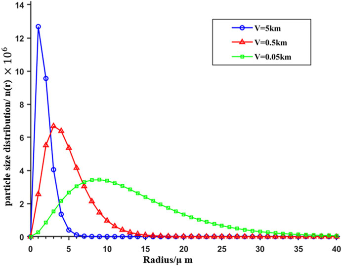
FIGURE 1. Solution process of vector radiation transmission equation based on RT3.

As can be seen from Figure 1, the relationship between the corresponding mode radius and particle size distribution varies for different visibility levels. The mode radius is between 0 and 1 μm, where the larger the visibility, the more the particle size distribution of sea spray particles and the larger the rising rate. The mode radius is between 0 and 3 μm, followed by the visibility of 0.5 km when the sea spray particle size distribution is more and rises faster; finally, when the visibility is 0.05 km, the mode radius is between 0 and 9 μm, the sea spray particle size distribution is more, and the trend is rising.

When the die radius >1 μm and visibility is 5 km, the particle size distribution decreases rapidly with the increase of die radius, and when the die radius reaches 6 μm, the sea mist particle distribution disappears; when the die radius >3 μm and visibility is 0.5 km, the particle size distribution decreases slowly with the increase of die radius, and when the die radius reaches 16 μm, the sea mist particle distribution disappears; when the die radius >9 μm and When the visibility is 0.05 km, the particle size distribution decreases slowly with the increase of the die radius, and the decreasing speed is slower than the first two, and the corresponding sea spray particle size distribution still exists when the die radius >24 μm.

3 Experiment

3.1 Experimental principle

3.1.1 Principle of liquid crystal tunable filter

The structure of the Liquid Crystal Tunable Filter (LCTF) is shown in Figure 2. The incident light passing through the LCTF crystal will form two coherent polarized beams, o-light and e-light, and the two beams will interfere to achieve transmission at a specific wavelength [11–17], and the intensity of the interference light coming out of the detector is

$I_0={\alpha }^2\left(1-{\mathit{sin}}^{2}2\alpha {\mathit{sin}}^2\frac{\delta }{2}\right)(5)$

Where a denotes the incident light amplitude, $\alpha$ is the angle between the fast axis of the crystal and the detector, and $\delta$ denotes the phase delay

$\delta =\frac{2\pi }{\lambda }\left|n_o-n_e\right|d(6)$

Where $\lambda$ is the wavelength, $n$ denotes the refractive index, and the crystal thickness is $d$. It can be seen that the light intensity changes with $\lambda$ and there is a great value of light intensity at a specific wavelength.

FIGURE 2

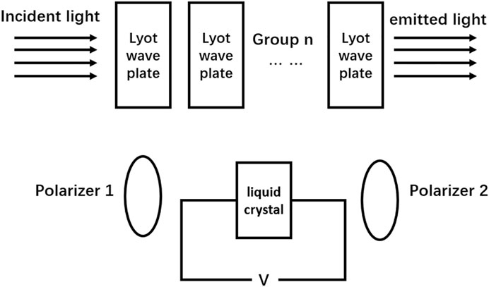
FIGURE 2. Schematic diagram of LCTF structure.

3.1.2 Principle of liquid crystal variable retarder

Liquid Crystal Variable Retarders (LCVR) are optical devices made based on the fact that anisotropic liquid crystal molecules with uniaxial birefringence properties are susceptible to deflection by electric and magnetic fields [18–21], thus causing the phase of the incident light wave to be modulated.

The basic principle of phase regulation in LCVR is shown in Figure 3 [22], where two transparent glasses are used as the upper and lower substrates, and Indium Tin Oxide is plated on the inner side of the substrate as the electrode so that the external signal is applied to the liquid crystal through the electrode. To pre-orient, the liquid crystal molecule pointing, an orientation film, usually polyimide, is also coated on the Indium Tin Oxide electrodes, which are encapsulated with liquid crystal spacers infused in between. When the driving voltage $U\le U_L$ is loaded on the LCVR ($U_L$ is the liquid crystal threshold voltage), as shown in Figure 3A, the long axis of the stretched anisotropic liquid crystal molecules is parallel to the substrate under the anchoring effect of the orientation film, and the long axis of the liquid crystal molecules is equivalent to the optical axis of a uniaxial crystal; when the driving voltage $U>U_L$ is loaded on the LCVR, the long axis of the liquid crystal molecules will follow the direction of the electric field under the action of the electric field as shown in Figure 3B, and the long axis of the liquid crystal molecules will be deflected along the electric field direction under the action of the electric field, which is equivalent to the deflection of the optical axis.

FIGURE 3

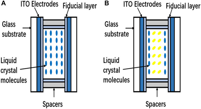
FIGURE 3. Principle diagram of Liquid Crystal Variable Retarder modulation. (A) $\mathit{U}\le {\mathit{U}}_{\mathit{L}}$ (B) $\mathit{U}>{\mathit{U}}_{\mathit{L}}$.

The relationship between the deflection angle θ of the optical axis and the driving voltage U is

$\theta =\left\{\begin{array}{c}0,\left(U\le U_L\right)\\ \frac{\pi }{2}-2\mathit{arctan}\left\{\mathit{exp}\left[{-\left(\frac{U-U_L}{U_0}\right)}^M\right]\right\},\left(U>U_L\right)\end{array}\right.(7)$

where $U_L$ is the threshold voltage and $U_0$, M are constants [23]. Due to the deflection of the long axis of the molecule, the angle $\alpha$ between the light vector K and the optical axis changes for the incident light wave, and the refractive index of e-light will change according to the birefringence property of anisotropic crystals. The refractive index of the e-light equation is

$n_e\left(\alpha \right)=\frac{n_o{n}_e}{{\left(n_0^2{\mathit{sin}}_{\alpha }^2+n_e^2{\mathit{cos}}_{\alpha }^2\right)}^{\raisebox{1ex}{$1$}\!\left/ \!\raisebox{-1ex}{$2$}\right.}}(8)$

Therefore, the phase delay of the modulated light through the Liquid Crystal Variable Retarder is

$\delta \left(\lambda ,\theta \right)=\frac{2\pi d}{\lambda }\left(n_e{-n}_o\right){\mathit{cos}}^2\theta (9)$

Where d is the thickness of the liquid crystal layer, and according to Eqs 7, 8, the refractive index of e-light differs at different places of the liquid crystal layer under the same driving voltage [24], thus making it imprecise to calculate the Liquid Crystal Variable Retarder phase delay using the theoretical equation [25], so the integration of Eq. 9 is

${\delta }_{LCVR}=\frac{2\pi }{\lambda }{\int }_0^d\left[n_e\left(\alpha \right)-n_o\right]dz(10)$

Where ${\delta }_{LCVR}$ is the phase delay of the LCVR. In an LCVR at a fixed voltage, the magnitude of phase delay is inversely related to the wavelength [26], the shorter the wavelength, the larger the amount of phase delay; the longer the wavelength, the smaller the amount of phase delay; at a fixed wavelength, the phase delay is positively related to the voltage, the larger the voltage the larger the phase delay.

The LCVR is a polarization optical device based on the fact that anisotropic liquid crystal molecules with uniaxial birefringence are easily deflected by electric and magnetic fields, thus modulating the phase of the incident light wave. Therefore, it is widely used in optical communication, optical information processing and polarization spectrum imaging.

3.2 Experimental setup and parameters of each setup

The visible light polarization imaging system is shown in Figure 4, where LCVR stands for Liquid Crystal Variable Retarder. LCTF stands for Liquid Crystal Tunable Filter. LCTF divides visible light into different wavelengths and produces light with different polarization states by changing the angle between the 2 LCVRs and imaging them. Literature 17 absorption spectra from individual textile fibers using LCTF, literature 21 developed a 400–1700 nm spectral polarization imager, and literature 26 developed a full Stokes parametric spectral polarization imager. None of the above articles have studied the factors affecting polarization imaging in depth, and the present device uses LCTF and LCVR to experiment and analyze the important factors affecting polarization imaging.

FIGURE 4

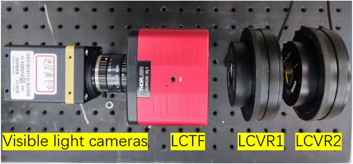
FIGURE 4. Spectral polarization imaging experimental setup.

The parameters of each instrument are shown in the following table. Table 1 shows the parameters of the visible light camera, Table 2 shows the parameters of the Liquid Crystal Tunable Filter, and Table 3 shows the parameters of the Liquid Crystal Variable Retarder.

TABLE 1

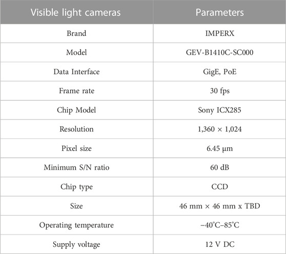
TABLE 1. Visible light camera Parameters.

TABLE 2

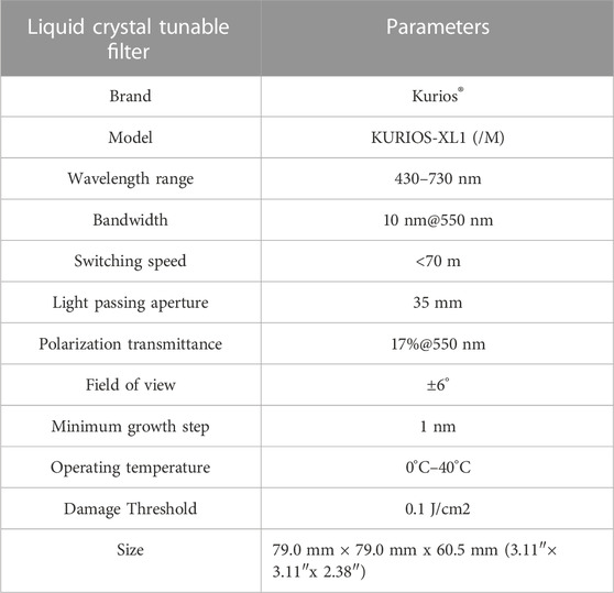
TABLE 2. Liquid crystal tunable filter parameters.

TABLE 3

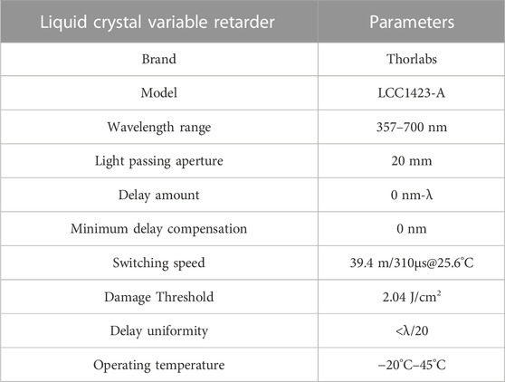
TABLE 3. Liquid crystal variable retarder parameters.

3.3 Liquid crystal variable retarder characteristic curve calibration experiment

The phase delay of the Liquid Crystal Variable Retarder (LCVR) is determined by the voltage applied to the liquid crystal, and we need to measure the voltage delay characteristics of the liquid crystal variable phase delayers used in the experiments. The LCVR made with anisotropic nematic liquid crystal molecules has a uniaxial birefringence effect, and when an external voltage is applied to the liquid crystal, the long axis of the liquid crystal molecules rotates at a different inclination angle due to the different electric field strengths. This changes the optical axis of the liquid crystal compared with the time when the electric field is not applied so that the light passing through the liquid crystal is modulated. The phase delay of LCVR The phase delay of LCVR is related to the applied driving voltage, and the LCVR phase delay characteristics are tested by the optical intensity method. The site of phase delay characteristics tested by the light intensity method is shown in Figure 5. Where LCVR stands for Liquid Crystal Variable Retarder.

FIGURE 5

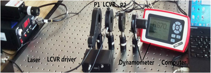
FIGURE 5. The site of phase delay characteristics tested by the light intensity method.

The LCVR device is placed between two orthogonal polarizers polarizer1 and polarizer2, the incident light source is a semiconductor laser of different wavelengths, the polarizer is a device made by THORLAB, the extinction ratio $ϵ={10}^{-5}$, the flux aperture is 20 mm, and the optical power meter is a product of Thorlabs.

Let the Mueller matrices of polarizer 1 and polarizer 2 be $M_{P1}\left({\beta }_1\right)$ and $M_{P2}\left({\beta }_2\right)$ respectively, the fast axis of the polarizer and the x-axis angle is ${\beta }_1$ and ${\beta }_2$ respectively, and the Mueller matrix of the LCVR device is $M_{LCVR}\left(\delta ,\theta \right)$, where the fast axis of LCVR and the x-axis angle $\theta$, the phase delay $\delta$.

$M_{LCVR}\left(\delta ,\theta \right)=\left[\begin{array}{cccc}1& 0& 0& 0\\ 0& {\mathit{cos}}^{2}2\theta +{\mathit{sin}}^{2}2\theta \mathit{cos}\delta & \mathit{cos}2\theta \mathit{sin}2\theta \left(1-\mathit{cos}\delta \right)& -\mathit{sin}2\theta \mathit{sin}\delta \\ 0& \mathit{cos}2\theta \mathit{sin}2\theta \left(1-\mathit{cos}\delta \right)& {\mathit{sin}}^{2}2\theta +{\mathit{cos}}^{2}2\theta \mathit{cos}\delta & \mathit{cos}2\theta \mathit{sin}\delta \\ 0& \mathit{sin}2\theta \mathit{sin}\delta & -\mathit{cos}2\theta \mathit{sin}\delta & \mathit{cos}\delta \end{array}\right](11)$

The relationship between the outgoing light Stokes vector $S_{out}$ and the incoming light Stokes vector $S_{in}$ is given by

$S_{out}=M_{P2}\left({\beta }_2\right)M\left(\theta ,\delta \right)M_{P1}\left({\beta }_1\right)S_{in}(12)$

Taking ${\beta }_2=0°$, ${\beta }_1=90°$, $\theta =45°$, then

$S_{out}=\frac{1}{4}\times \left[\begin{array}{cccc}1& 1& 0& 0\\ 1& 1& 0& 0\\ 0& 0& 0& 0\\ 0& 0& 0& 0\end{array}\right]\times \left[\begin{array}{cccc}1& 0& 0& 0\\ 0& \mathit{cos}\delta & 0& -\mathit{sin}\delta \\ 0& 0& 1& 0\\ 0& \mathit{sin}\delta & 0& \mathit{cos}\delta \end{array}\right]\times \left[\begin{array}{cccc}1& -1& 0& 0\\ -1& 1& 0& 0\\ 0& 0& 0& 0\\ 0& 0& 0& 0\end{array}\right]{\times S}_{in}(13)$

Then the relationship between the outgoing light intensity I and the amount of phase delay $\delta$ is

$I=0.5I_{\mathit{max}}\left(1-\mathit{cos}\delta \right)(14)$

Where, $I_{\mathit{max}}$ is the maximum light intensity value of the outgoing light.

The measured LCVR drive voltage versus phase delay amount characteristic curve is shown in Figure 6, where the horizontal coordinate represents the LCVR drive voltage and the vertical coordinate represents the phase delay amount.

FIGURE 6

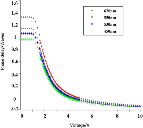
FIGURE 6. Liquid Crystal Variable Retarder phase delay characteristic curve.

3.4 Experiments on the effect of different visibility on polarization imaging

For light fog (visibility 5 km), medium fog (visibility 0.5 km) and dense fog (0.05 km) three typical visibility conditions to carry out polarization imaging experiments, imaging of a building 4 km away, the experimental results are as follows, Figure 7 shows the intensity image under different visibility, Figure 9 shows the polarization image under different visibility.

FIGURE 7

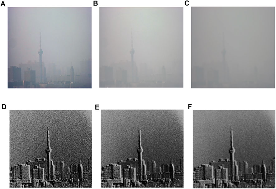
FIGURE 7. Intensity and Polarization images at different visibility levels. (A) Intensity image (visibility 5 km) (B) Intensity image (visibility 0.5 km) (C) Intensity image (0.05 km) (D) Polarization image (visibility 5 km) (E) Polarization image (visibility 0.5 km) (F) Polarization image (0.05 km).

The histogram of contrast between the intensity image and the polarization image is shown in Figure 8.

FIGURE 8

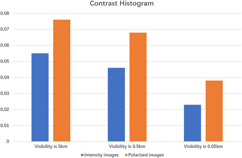
FIGURE 8. Histogram of contrast between intensity image and polarization image.

As can be seen from Figure 8, the contrast ratio of the intensity image is 5.5% and the contrast ratio of polarization is 7.6% at the visibility of 5 km, which is 1.38 times better; the contrast ratio of the intensity image is 4.4% and the contrast ratio of polarization is 6.3% at the visibility of 0.5 km, which is 1.43 times better; the contrast ratio of intensity image is 2.3% and the contrast ratio of polarization at the visibility of 0.05 km is 3.8%, an improvement of 1.65 times. The contrast of the polarized image is higher than that of the intensity image at all three visibility levels, which shows that the polarized image can effectively suppress stray light caused by atmospheric particle scattering and effectively improve the image contrast; as the visibility decreases, the image contrast of the polarized image decreases. As the average radius of particles increases when the visibility decreases, the particle concentration increases, which leads to more scattering, while the scattering effect between particles leads to depolarization, which reduces the polarization so that the polarization decreases gradually as the visibility decreases.

3.5 Experiment with the effect of different wavelengths on polarization imaging

To study the effect of different wavelengths on polarization imaging, we selected three wavelengths, 450 nm, 530 nm and 670 nm, to carry out spectral polarization imaging experiments, imaging of a building 4 km away, and the experimental results are as follows. Figure 9 shows the intensity polarization images of the three wavelengths.

FIGURE 9

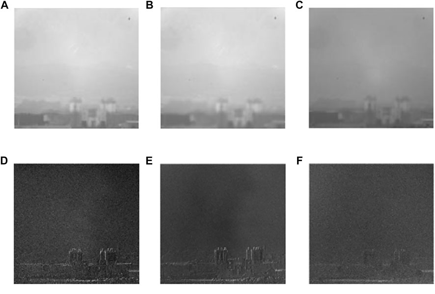
FIGURE 9. Intensity and Polarization images of three wavelengths (A) 670 nm Intensity image (B) 530 nm Intensity image (C) 450 nm Intensity image. (D) 670 nm Polarization image (E) 530 nm Polarization image (F) 450 nm Polarization image.

The histogram of contrast between the intensity image and the polarization image is shown in Figure 10.

FIGURE 10

FIGURE 10. Intensity image and polarization image contrast histogram.

As visualized in Figure 9, the intensity image is blurred, the imaging gray value is high, a lot of information is covered, the contour details are not obvious enough, and the target edge information cannot be seen, which is due to the different absorption and scattering effects of sea fog particles on different wavelengths of light in the complex sea fog environment, resulting in more background noise during imaging. There is a significant difference in the grayscale values of the polarized images compared to the conventional intensity images.

Figure 10 shows that at 670 nm, the intensity image contrast is 8.1% and the polarization image contrast is 9.3%, an improvement of 1.15 times; at 530 nm, the intensity image contrast is 7.0% and the polarization image contrast is 9.0%, an improvement of 1.29 times; at 450 nm, the intensity image contrast is 6.4% and the polarization image contrast is 7.5%, a The improvement was 1.17 times. The image contrast of polarization imaging at all three wavelengths is higher than that of intensity images, and the image contrast decreases as the wavelength decreases. Among the three wavelengths, the difference between the target and the background is the largest at 670 nm, which is more suitable for the observation of the target.

3.6 Experiments on the effect of different imaging distances on polarization imaging

To study the effect of different imaging distances on polarization imaging, we selected 50 m, 1.5 km at the tower crane and 100 m, 2.5 km at the house to carry out spectral polarization imaging experiments, the experimental results are as follows, Figure 11 is the intensity image and polarization degree of the four imaging distances.

FIGURE 11

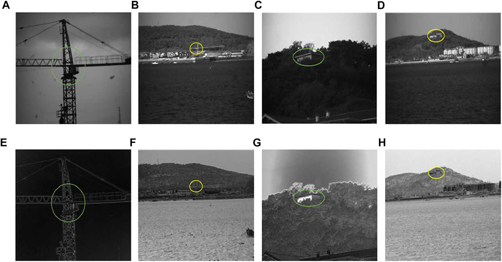
FIGURE 11. Intensity and Polarization images for different imaging distances (A) 50 m Intensity image (B) 1.5 km Intensity image (C) 100 m Intensity image (D) 2.5 km Intensity image (E) 50 m Polarization image (F) 1.5 km Polarization image (G) 100 m Polarization image (H) 2.5 km Polarization image.

The histograms of the intensity image and polarization image contrast for different imaging distances are shown in Figure 12.

FIGURE 12

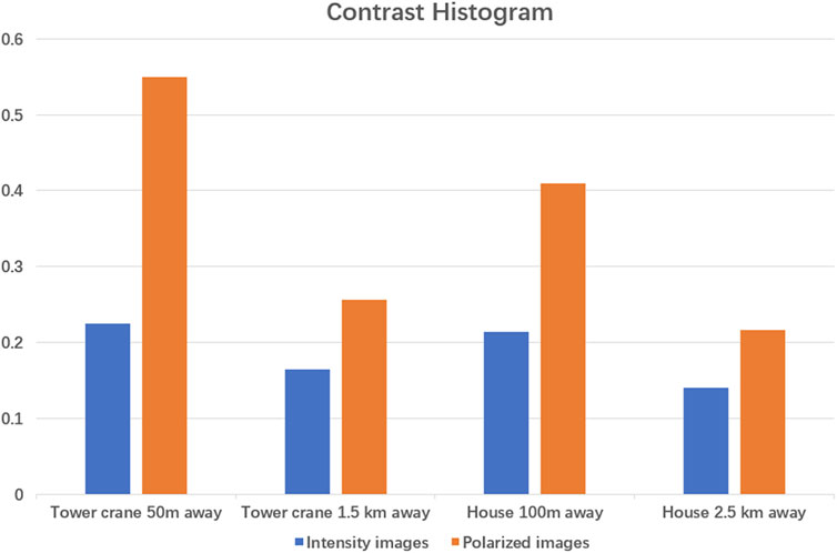
FIGURE 12. Histogram of contrast between images with different imaging distance intensity and polarized images.

As can be seen in Figure 12, the intensity image contrast of the tower crane at 50 m away is 22.5% and the polarization contrast is 55%, which is 2 times higher; the intensity image contrast of the tower crane at 1.5 km away is 14% and the polarization contrast is 21.6%, which is 1.54 times higher; the intensity image contrast of the house at 100 m away is 21.4% and the polarization contrast is 41%, which is 1.92 times higher; the intensity image contrast of the house at 2.5 km away is 16.5% and the polarization contrast is 25.6%, which is 1.55 times higher. The contrast of the intensity image of the house 2.5 km away was 16.5%, and the polarization contrast was 25.6%, which improved 1.55 times; the contrast of the polarization image was higher than that of the intensity image; for the same object, the contrast of both the intensity image and the polarization image decreased with the increase of the imaging distance.

4 Conclusion

In this paper, we designed a multispectral polarization detection imaging system to study the effects of different visibility, different wavelengths and different imaging distances on the imaging effect. Because when the visibility decreases, increased particle concentration leads to more scattering, and the scattering effect between particles leads to depolarization, thus reducing the polarization, therefore, the polarization will gradually decrease with the decrease of visibility. Under the three wavelengths, the 670 nm imaging effect is the best. The closer the imaging distance, the better the imaging effect. According to the calculated contrast, the polarized image has obvious advantages over conventional intensity imaging; the texture details that cannot be seen in the intensity imaging can be well seen in the polarized image. Therefore, when the polarization imaging detection technique is used to detect targets in a sea fog environment, the target contrast can be effectively improved. Polarization imaging can enrich target information, improve image quality and target detection accuracy, and can better analyze the polarized light information reflected from the object’s surface, the roughness, texture and edge information of the target can be obtained, which can improve the recognition of the target and the contrast between the target and the background to a certain extent, which is very effective in target recognition in complex environments such as sea fog.

Data availability statement

The original contributions presented in the study are included in the article/Supplementary Material, further inquiries can be directed to the corresponding author.

Author contributions

Data curation, QF and YZ; formal analysis, LS and KL; investigation, JZ and SZ; methodology, QF; project administration, YZ and KL; resources, QF; software, WY and JZ; supervision, MZ and LS; validation, SZ; visualization, MZ and WY; writing—original draft, QF; writing—review and editing, WY All authors have read and agreed to the published version of the manuscript.

Funding

National Natural Science Foundation of China (No. 61890963; No. 61890960; No. 62127813).

Acknowledgments

Thanks to the Natural Science Foundation of China for helping identify collaborators for this work.

Conflict of interest

The authors declare that the research was conducted in the absence of any commercial or financial relationships that could be construed as a potential conflict of interest.

Publisher’s note

All claims expressed in this article are solely those of the authors and do not necessarily represent those of their affiliated organizations, or those of the publisher, the editors and the reviewers. Any product that may be evaluated in this article, or claim that may be made by its manufacturer, is not guaranteed or endorsed by the publisher.

References

1. Zhang C, Zhang J, Wu X, Huang M. Numerical analysis of light reflection and transmission in poly-disperse sea fog. Opt Express (2020) 28(17):25410–30. doi:10.1364/oe.400002

PubMed Abstract | CrossRef Full Text | Google Scholar

2. Liu Y, Fu Q, Zhang S, Zhan J, Shi H, Li Y, et al. Polarization pattern of skylight in multi-layer environment of atmosphere and Sea Fog[J]. Acta Armamentarii (2022) 43(5):1201–7.

Google Scholar

3. Fu Q, Luo K, Song Y, Zhang M, Zhang S, Zhan J, et al. Study of Sea Fog environment polarization transmission characteristics. Appl Sci (2022) 12:8892. doi:10.3390/app12178892

CrossRef Full Text | Google Scholar

4. Wang F, Yin C, Wang Y. Research of polarization imaging detection method for water surface target in foggy weather[C]//International Symposium on Photoelectronic Detection and Imaging 2013: Infrared Imaging and Applications. SPIE (2013) 8907:1078–86.

Google Scholar

5. Fu Q, Liu Y, Liu N, Si L, Zhang S, Zhan J, et al. Sky polarization pattern under multi-layer environment of atmosphere and sea fog. Front Phys (2022) 10:994. doi:10.3389/fphy.2022.1036560

CrossRef Full Text | Google Scholar

6. Fade J, Panigrahi S, Carré A, Frein L, Hamel C, Bretenaker F, et al. Long-range polarimetric imaging through fog. Appl Opt (2014) 53:3854–65. doi:10.1364/ao.53.003854

PubMed Abstract | CrossRef Full Text | Google Scholar

7. Li S, Jiang H, Zhu J, Duan J, Fu Q, Fu Y, et al. Current status and key technologies of polarization imaging detection technology[J]. China Opt (2013) 6(06):803–9.

Google Scholar

8. Chen Y, Zeng Y, Pan Y, Zhao Y. A new method for military dummy target identification[J]. Electron Des Eng (2011) 19(16):89–92.

Google Scholar

9. Al Naboulsi MC, Sizun H, de Fornel F. Fog attenuation prediction for optical and infrared waves. Opt Eng (2004) 43(2):319–29. doi:10.1117/1.1637611

CrossRef Full Text | Google Scholar

10. Jiang Z. The relationship between water content, temperature and visibility in clouds[J]. Meteorol Mon (1994) 20(10):40–1. [J].

Google Scholar

11. Liu Z. Research on target detection technology based on visible light polarization imaging[D]. Beijing, China: Graduate School of Chinese Academy of Sciences (2016).

Google Scholar

12. Morris HR, Hoyt CC, Miller P, Treado PJ. Liquid crystal tunable filter Raman chemical imaging. Appl Spectrosc (1996) 50(6):805–11. doi:10.1366/0003702963905655

CrossRef Full Text | Google Scholar

13. Stratis DN, Eland KL, Carter JC, Tomlinson SJ, Angel SM. Comparison of acousto-optic and liquid crystal tunable filters for laser-induced breakdown spectroscopy. Appl Spectrosc (2001) 55(8):999–1004. doi:10.1366/0003702011953144

CrossRef Full Text | Google Scholar

14. Filters VSLCT. VariSpec liquid crystal tunable filters[J]. Massachusetts: Photonics Spectra (2006).

Google Scholar

15. Wierzbicki D, Wilinska M (2014). Liquid crystal tunable filters in detecting water pollution[C]//Environmental Engineering, In Proceedings of the International Conference on Environmental Engineering. ICEE, New York, NY: Vilnius Gediminas Technical University, Department of Construction Economics and Property.

Google Scholar

16. Stevenson BP, Kendall WB, Stellman CM, Olchowski FM PHIRST light: a liquid crystal tunable filter hyperspectral sensor proceedings: Proc. SPIE 5093, Algorithms and Technologies for Multispectral, Hyperspectral, and Ultraspectral Imagery IX, September 23, 2003 doi:10.1117/12.497540

CrossRef Full Text | Google Scholar

17. Markstrom LJ, Mabbott GA. Obtaining absorption spectra from single textile fibers using a liquid crystal tunable filter microspectrophotometer. Forensic Sci Int (2011) 209(1-3):108–12. doi:10.1016/j.forsciint.2011.01.014

PubMed Abstract | CrossRef Full Text | Google Scholar

18. Gisler D, Feller A, Gandorfer AM. Achromatic liquid crystal polarization modulator[J]. Proc SPIE (2003) 4843:45–54.

Google Scholar

19. Gladish JC, Duncan D. Parameterizing liquid crystal variable retarder structural organization with a fractal-Born approximation model. Opt Eng (2016) 55(5):054104–8. doi:10.1117/1.oe.55.5.054104

CrossRef Full Text | Google Scholar

20. Xiao XF, Voelz D, Sugiura H. Field of view characteristics of a liquid crystal variable retarder[J]. SPIE (2003) 5158:142–50.

Google Scholar

21. Gupta N Development of Spectro polarimetric Imagers from 400 to 1700 nm[J]. in Proc of SPIE (2014). 90990N.

Google Scholar

22. Li K, Wang Z, Zhang R, Yu H. Study on birefringent dispersion of liquid crystal variable delayers[J]. China Laser (2015) 42:232–46. doi:10.1016/j.chieco.2014.04.005

CrossRef Full Text | Google Scholar

23. Jiang J, Zhang D, Li J. Development of liquid crystal variable delay device and electronically controlled phase delay measurement[J]. Laser Tech (2011) 35:652–3.

Google Scholar

24. Saleh BEA, Lu K. Theory and design of the liquid crystal TV as an optical spatial phase modulator. Opt Eng (1990) 29(3):240–6. doi:10.1117/12.55584

CrossRef Full Text | Google Scholar

25. Xiao D, Wang M. Crystal physics [M]. Chengdu: Sichuan University Press (1989). p. 146–7.

Google Scholar

26. Yang F, Li Y, Hu B, Kong L, Wei R, Li H. Design of polarization hyperspectral imaging system based on LCTF and LCVR[J]. Spectrosc Spectral Anal (2017) 37(08):2610–4.

Google Scholar