Quantum field theory for coherent photons: isomorphism between Stokes parameters and spin expectation values

1 Introduction

Stokes and Poincaré successfully established a systematic way to describe polarisation of lights by using several real value parameters, known as Stokes parameters, which are described as a vector on the Poincaré sphere [1–5]. This is a spectacular achievement at the time, because it was before the discoveries of Plank and Einstein, that lights are composed of a quanta, named a photon, with both particle and wave characters to establish quantum mechanics [6–9]. It is intriguing to learn from words of Einstein [10], quote, All these 50 years of conscious brooding have brought me no nearer to the answer to the question, “What are light quanta?”, unquote.

Here, we revisit a lemma of this grand challenge: What is spin of a photon? Our answer to this question is polarisation. One might think this is obvious and already well-established, but it is less obvious, because it is generally believed that the total angular momentum of a photon is impossible to split [11] into spin and orbital angular momentum [4,5,12–17] in a unique gauge invariant way [11,13–15,18]. It is beyond the scope of this paper to address this mystery [19,20], however, we will focus on understanding the spin of a photon. We are interested in a monochromatic coherent ray of photons emitted from a laser source, such that we will investigate low-energy condensed-matter physics and we will not deal with the Lorentz invariance, required for high-energy physics. The optical spin angular momentum was previously obtained by using many-body number operators, but it was shown that the operators are commutable [13,15]. Therefore, the quantum-mechanical nature of the spin of a photon is still not completely understood, yet.

We think some of these issues are coming from various ways to define the polarisation states of lights [21–24], spreading among literature. Unfortunately, there is no unique standard for the definitions, because the way to define rotation depends on whether we are evaluating the polarisation state seen from the light-source side or from the detector side. It is also different among physicists and engineers whether we are going to use the phase evolution as e^i(kz−ωt), which is common for physicists, or alternatively, as e^i(ωt−kz), which is more often used for engineers, where the parameters are time (t), the spatial axis along the direction of the propagation (z), the wavenumber (k), and the angular frequency (ω), as usual. Depending on this phase evolution over t and z, the direction of the rotation of the polarisation state will be changed. These differences impose unnecessary confusions among researchers for considering the polarisation states of lights. Therefore, we have summarised our preferential definition in Supplementary Material. Our convention is similar to the classical textbook of Jackson [4], but it is not necessarily common.

Spin is an intrinsic degree of freedom, inherent to an elementary particle. A photon has spin 1 in the unit of Dirac constant (ℏ), and it is described by Bose statistics, because of this integer spin [6–9]. For an elementary particle of spin 1, in principle, there exists 3 major components to describe the polarisation state as fundamental basis states for Lie-algebra, however, one of the component with zero spin component is not observable [9,25]. This is coming from the fact that the lights are transverse waves, which is fundamentally coming from the theory of relativity, based on the principle that there is no rest frame for a photon, which is travelling at the speed of light c) in a vacuum [25–27]. Consequently, the spin state of a photon can be described by Lie-algebra of spin 1/2 [3,5,7,8,28–40].

The purpose of this work is to clarify the correlation between the classical description of polarisation states by using Stokes parameters in Poincaé sphere and a many-body description of spin. We show that the vector described by Stokes parameters is actually the quantum-mechanical expectation value of spin operators. This means that the Stokes parameters are order parameters to describe a coherent state of a ray from a laser, which is essentially composed of a single mode with macroscopic number of photons degenerated due to the Bose-Einstein condensation of photons. We also show the equivalence of Poincaé sphere with Bloch sphere, and explain how classical results for polarisation with various parameters such as orientation angle (Ψ), ellipticity angle (χ), auxiliary angle (α), and phase (δ), are all derived from simple geometrical consideration on these spheres. We also show that the change of the basis states are equivalent to the rotation in the special unitary of degree two (SU(2)) Hilbert space to describe the polarisation state. Our results show that it is quite natural to believe that the spin operators are essentially equivalent to Stokes operators, which reasonably work as standard quantum-mechanical angular momentum operators. Angular momentum is an observable to characterise a polarisation state on the Poincaré sphere, satisfying commutation relationship, working as a generator of rotation, and describing the polarisation state of a coherent state of photons.

2 Principles

2.1 Coherent state

A photon is an elementary particle and it must follow the principle of quantum mechanics [6–9]. A photon can be created in a laser source, or it can be annihilated in a detector. The creation and annihilation are described by operators ${\widehat{a}}_{\sigma }^{†}$ and ${\widehat{a}}_{\sigma }$, respectively, which satisfy the commutation relationships for Bose particles [9,16,41,42] as $[{\widehat{a}}_{\sigma },{\widehat{a}}_{{\sigma }^{\prime }}]=0$, $[{\widehat{a}}_{\sigma }^{†},{\widehat{a}}_{{\sigma }^{\prime }}^{†}]=0$, and $[{\widehat{a}}_{\sigma },{\widehat{a}}_{{\sigma }^{\prime }}^{†}]={\delta }_{\sigma ,{\sigma }^{\prime }}$, where σ stands for the polarisation states such as σ = H for horizontally polarised state and σ = V for vertically polarised state. δ_σ,σ′ is the Kronecker delta, which becomes 1 if the polarisation states of σ and σ′ coincide, and 0 if the polarisation states are orthogonal. We can also choose another orthogonal base such as linearly polarised states along diagonal (σ = D) and anti-diagonal (σ = A) directions, or left (σ = L) and right (σ = R) circularly-polarised states (Supplementary Material).

We are interested in a monochromatic coherent ray of photons propagating in a material such as a waveguide or an optical fibre or in a vacuum, emitted from a laser source [5], because lasers are ubiquitously available. The coherent states [16,41,42] are described as |α_H, α_V⟩ = |α_H⟩|α_V⟩, where.

$|{\alpha }_{\text{H}}\rangle ={\mathrm{e}}^{-\frac{|{\alpha }_{\text{H}}{|}^2}{2}}{\mathrm{e}}^{{\alpha }_{\text{H}}{\widehat{a}}_{\text{H}}^{†}}|0\rangle (1)$

$|{\alpha }_{\text{V}}\rangle ={\mathrm{e}}^{-\frac{|{\alpha }_{\text{V}}{|}^2}{2}}{\mathrm{e}}^{{\alpha }_{\text{V}}{\widehat{a}}_{\text{V}}^{†}}|0\rangle ,(2)$

for which we assign ${\alpha }_{\text{H}}=\sqrt{N_{\text{H}}}=\sqrt{N}\cos \alpha$, ${\alpha }_{\text{V}}=\sqrt{N_{\text{V}}}{\mathrm{e}}^{i\delta }=\sqrt{N}\sin \alpha {\mathrm{e}}^{i\delta }$ with the average number of photons for each polarisation given by N_H and N_V, and the total number of photons in the system is N = N_H + N_V. The auxiliary angle of α is the angle to split the electric field between horizontal and vertical directions (Supplementary Material) and the relative phase of δ = δ_y − δ_x is the amount of the phase shift for the vertical direction (δ_y), measured from that for the horizontal direction (δ_x). The coherent states have important characteristics.

${\widehat{a}}_{\text{H}}|{\alpha }_{\text{H}}\rangle ={\alpha }_{\text{H}}|{\alpha }_{\text{H}}\rangle (3)$

${\widehat{a}}_{\text{V}}|{\alpha }_{\text{V}}\rangle ={\alpha }_{\text{V}}|{\alpha }_{\text{V}}\rangle ,(4)$

which mean these are eigenstates of annihilation operators.

We consider the following complex electric field operator, defined as,

$\widehat{\mathcal{E}}\left(z,t\right)=\sqrt{\frac{2\hslash \omega }{ϵV}}{\mathrm{e}}^{i\beta }\left({\widehat{a}}_{\text{H}}\widehat{\mathbf{x}}+{\widehat{a}}_{\text{V}}\widehat{\mathbf{y}}\right),(5)$

where β = kz − ωt + δ_x, $\widehat{\mathbf{x}}$ and $\widehat{\mathbf{y}}$ are unit vectors along x and y directions, respectively, ϵ is the dielectric constant of the material, and V is the volume of the system. In a uniform material of the refractive index n, the dispersion is simply obtained as ω = vk = ck/n by solving the Maxwell equations (4) and (5). By applying $\widehat{\mathcal{E}}(z,t)$ to |α_H, α_V⟩ from the left, we obtain

$\widehat{\mathcal{E}}\left(z,t\right)|{\alpha }_{\text{H}},{\alpha }_{\text{V}}\rangle =\mathcal{E}\left(z,t\right)|{\alpha }_{\text{H}},{\alpha }_{\text{V}}\rangle ,(6)$

which means the coherent state is an eigenstate of this operator and the operation did not change the state except for the factor, $\mathcal{E}(z,t)$, which gives the complex amplitude of the electric field as

$\mathcal{E}\left(z,t\right)=\left(\begin{array}{c}\hfill {\mathcal{E}}_x\hfill \\ \hfill {\mathcal{E}}_y\hfill \end{array}\right)=E_0{\mathrm{e}}^{i\beta }\left(\begin{array}{c}\hfill \cos \alpha \hfill \\ \hfill \sin \alpha {\mathrm{e}}^{i\delta }\hfill \end{array}\right),(7)$

with the amplitude of $E_0=\sqrt{2\hslash \omega N/(ϵV)}$. Therefore, $\widehat{\mathcal{E}}(z,t)|{\alpha }_{\text{H}},{\alpha }_{\text{V}}\rangle$ also works as a wavefunction to describe the coherent state of photons. Then, we recognise that $\mathcal{E}(z,t)$ is actually a spinor representation of the wavefunction, and it is indeed rewritten as

$\mathcal{E}\left(z,t\right)=E_0\mathrm{\Psi }\left(z,t\right)|\mathrm{J}\mathrm{o}\mathrm{n}\mathrm{e}\mathrm{s}\rangle ,(8)$

where Ψ(z, t) = e^iβ is the orbital part of the wavefunction, and |Jones⟩ it the Jones vector to describe the polarisation states (Supplementary Material). Therefore, the Jones vector is actually the wavefunction itself to describe the spin state of the coherent photons, quantum mechanically. It is interesting to note that the many-body coherent state is described simply by a single mode of Ψ(z, t) with the spin state as inherent internal degrees of freedom. This is coming from the nature of the Bose-Einstein condensation for the coherent laser beam, in which macroscopic number of photons are degenerate to occupy the single mode.

In a real material with a specific geometrical structure, patterned into a form of a waveguide or a fibre, we must solve the Helmholtz equation

${\nabla }^2\mathrm{\Psi }\left(\mathbf{r}\right)={\mu }_0ϵ\left(\mathbf{r}\right)\frac{{\partial }^2}{\partial t^2}\mathrm{\Psi }\left(\mathbf{r}\right),(9)$

because the dielectric constant has a profile in the form of ϵ = ϵ(r), due to the spacial distribution of material compositions. We are aware that this is very important to take into account for the more realistic considerations. By respecting the symmetry of the waveguide [43], we can also consider various forms of the orbital wavefunction, including the vortex nature of the beam with orbital angular momentum [4,5,12–17]. Here, we consider only the plane wave solution of the Helmholtz equation as Ψ(z, t) = e^iβ, which makes a lot of serious problems for separating the spin and orbital parts of the angular momentum [11,13–15,18], as we shall see briefly below. Nevertheless, the plane wave solution makes calculations easy, such that it is still useful for a theoretical perspective.

We also note that $\widehat{\mathcal{E}}(z,t)$ is not observable, since all physical observables must be real. In order to observe the electric field, which is observable, we must define the real electric field operator given by

$\widehat{\mathbf{E}}=\frac{1}{2}\left(\widehat{\mathcal{E}}+{\widehat{\mathcal{E}}}^{†}\right).(10)$

If we take the quantum-mechanical average over the coherent state, we obtain.

$\mathbf{E}\left(z,t\right)=\langle \widehat{\mathbf{E}}\rangle (11)$

$=\langle {\alpha }_{\text{H}},{\alpha }_{\text{V}}|\widehat{\mathbf{E}}|{\alpha }_{\text{H}},{\alpha }_{\text{V}}\rangle (12)$

$=E_0\left(\cos \alpha \cos \beta \widehat{\mathbf{x}}+\sin \alpha \cos \left(\beta +\delta \right)\widehat{\mathbf{y}}\right)(13)$

$=\mathfrak{R}\left(\mathcal{E}\left(z,t\right)\right),(14)$

which is indeed real. Please also note that the application of $\widehat{\mathbf{E}}$ to |α_H, α_V⟩ changes the original state, because the coherent state is not the eigenstate of the creation operator [16,41,42]. Therefore, it is essential to treat the electric field by using a complex value rather than real value, so that the use of a complex value is not a mere mathematical convention. The wavefunction is intrinsically described by a complex value for a photon, just like the other quantum-mechanical systems [6–9].

We can also obtain the quantum-mechanical average of the energy for the photons.

${\bar{U}}_{\text{QM}}=\frac{V}{2}⟨\overline{\widehat{\mathbf{E}}\cdot \widehat{\mathbf{D}}}+\overline{\widehat{\mathbf{B}}\cdot \widehat{\mathbf{H}}}⟩=ϵV⟨\overline{\widehat{\mathbf{E}}\cdot \widehat{\mathbf{E}}}⟩(15)$

$=\frac{ϵV}{4}⟨\stackrel{̄}{\widehat{\mathcal{E}}\cdot \widehat{{\mathcal{E}}^{†}}}+\stackrel{̄}{\widehat{{\mathcal{E}}^{†}}\cdot \widehat{\mathcal{E}}}+\overline{\widehat{\mathcal{E}}\cdot \widehat{\mathcal{E}}}+\stackrel{̄}{\widehat{{\mathcal{E}}^{†}}\cdot \widehat{{\mathcal{E}}^{†}}}⟩(16)$

$=\frac{ϵV}{4}⟨\stackrel{̄}{\widehat{\mathcal{E}}\cdot \widehat{{\mathcal{E}}^{†}}}+\stackrel{̄}{\widehat{{\mathcal{E}}^{†}}\cdot \widehat{\mathcal{E}}}⟩(17)$

$=\frac{ϵV}{4}\frac{2\hslash \omega }{ϵV}⟨{\widehat{a}}_{\text{H}}^{†}{\widehat{a}}_{\text{H}}+{\widehat{a}}_{\text{H}}{\widehat{a}}_{\text{H}}^{†}+{\widehat{a}}_{\text{V}}^{†}{\widehat{a}}_{\text{V}}+{\widehat{a}}_{\text{V}}{\widehat{a}}_{\text{V}}^{†}⟩(18)$

$=\hslash \omega ⟨{\widehat{a}}_{\text{H}}^{†}{\widehat{a}}_{\text{H}}+\frac{1}{2}+{\widehat{a}}_{\text{V}}^{†}{\widehat{a}}_{\text{V}}+\frac{1}{2}⟩(19)$

$=\hslash \omega \left(N_{\text{H}}+\frac{1}{2}+N_{\text{V}}+\frac{1}{2}\right)(20)$

$=\hslash \omega \left(N+1\right),(21)$

where the bar stands for the t average, and 1/2 is coming from the zero-point oscillations.

2.2 Electro-magnetic field operators for lasers

We will obtain various electro-magnetic field operators to describe a coherent ray of photons emitted from a laser. We use a Coulomb gauge, which satisfy

$\mathbf{\nabla }\cdot \widehat{\mathbf{A}}=0,(22)$

where $\widehat{\mathbf{A}}$ is the vector potential operator. The magnetic induction operator, $\widehat{\mathbf{B}}$, and $\widehat{\mathbf{E}}$ are obtained from $\widehat{\mathbf{A}}$, as.

$\widehat{\mathbf{B}}=\nabla \times \widehat{\mathbf{A}}=\frac{\mathbf{k}\times \widehat{\mathbf{E}}}{\omega }(23)$

$\widehat{\mathbf{E}}=-{\partial }_t\widehat{\mathbf{A}},(24)$

respectively. Alternatively, we have already obtained $\widehat{\mathbf{E}}$ as,

$\widehat{\mathbf{E}}=\sqrt{\frac{\hslash \omega }{2ϵV}}\left(\left({\widehat{a}}_{\text{H}}{\mathrm{e}}^{i\beta }+{\widehat{a}}_{\text{H}}^{†}{\mathrm{e}}^{-i\beta }\right)\widehat{\mathbf{x}}+\left({\widehat{a}}_{\text{V}}{\mathrm{e}}^{i\beta }+{\widehat{a}}_{\text{V}}^{†}{\mathrm{e}}^{-i\beta }\right)\widehat{\mathbf{y}}\right),(25)$

we can obtain $\widehat{\mathbf{A}}$, instead, as

$\widehat{\mathbf{A}}=\frac{-i}{\omega }\sqrt{\frac{\hslash \omega }{2ϵV}}\left(\left({\widehat{a}}_{\text{H}}{\mathrm{e}}^{i\beta }-{\widehat{a}}_{\text{H}}^{†}{\mathrm{e}}^{-i\beta }\right)\widehat{\mathbf{x}}+\left({\widehat{a}}_{\text{V}}{\mathrm{e}}^{i\beta }-{\widehat{a}}_{\text{V}}^{†}{\mathrm{e}}^{-i\beta }\right)\widehat{\mathbf{y}}\right).(26)$

Consequently, we obtain

$\widehat{\mathbf{B}}=\frac{1}{v}\sqrt{\frac{\hslash \omega }{2ϵV}}\left(\left({\widehat{a}}_{\text{H}}{\mathrm{e}}^{i\beta }+{\widehat{a}}_{\text{H}}^{†}{\mathrm{e}}^{-i\beta }\right)\widehat{\mathbf{y}}-\left({\widehat{a}}_{\text{V}}{\mathrm{e}}^{i\beta }+{\widehat{a}}_{\text{V}}^{†}{\mathrm{e}}^{-i\beta }\right)\widehat{\mathbf{x}}\right).(27)$

Here, we assumed that the ray is described by a single mode, which is remarkably different from a standard description of the $\widehat{\mathbf{E}}$ and $\widehat{\mathbf{B}}$ in a Quantum Electro-Dynamics (QED) theory [6,9,16,41,42], for which the sum over all possible modes with different wavelengths are included. For the application of a coherent ray from lasers, the single mode are dominated over other modes [5]. We can easily extend the theory to include a few modes for describing propagation of multiple modes just by summing up these contributions based on a superposition principle. But, the main point here is the Bose-Einstein condensation character of the coherent ray, and we do not have to consider infinite number of electromagnetic fields in a vacuum. In that sense, our system, considering here for a standard optical laser lab, is remarkably different from situations in high energy physics, where the Lorentz invariance is inevitable [11,14,18]. In a waveguide, the spatial symmetry is broken a priori, such that the orbital is not uniform, reflecting the shape and the profile of the material compositions [43].

The momentum operator of the electro-magnetic field, ${\widehat{\mathbf{p}}}_{\text{field}}$, is given from the Poynting vector operator, $\widehat{\mathbf{S}}=\widehat{\mathbf{E}}\times \widehat{\mathbf{H}}$, with the magnetic field operator of $\widehat{\mathbf{H}}$, as

${\widehat{\mathbf{p}}}_{\text{field}}=ϵ\left(\widehat{\mathbf{E}}\times \widehat{\mathbf{B}}\right)=ϵ{\mu }_0\left(\widehat{\mathbf{E}}\times \widehat{\mathbf{H}}\right)=\frac{1}{v^2}\widehat{\mathbf{S}},(28)$

where μ₀ is the permeability of a material, which is usually almost the same as that in a vacuum [5] for most of the optical materials, except for optical isolators. By integrating over V, we obtain

${\widehat{\mathbf{P}}}_{\text{field}}=\hslash k\widehat{\mathbf{z}}\left(\left({\widehat{a}}_{\text{H}}^{†}{\widehat{a}}_{\text{H}}+\frac{1}{2}\right)+\left({\widehat{a}}_{\text{V}}^{†}{\widehat{a}}_{\text{V}}+\frac{1}{2}\right)\right),(29)$

for which we have used

$\sqrt{\frac{\hslash \omega }{2ϵV}}\frac{1}{v}\sqrt{\frac{\hslash \omega }{2ϵV}}\frac{1}{v^2{\mu }_0}V=\frac{1}{v}\frac{\hslash \omega }{2}\frac{1}{v^2ϵ{\mu }_0}=\frac{\hslash k}{2}(30)$

for the factor, $\widehat{\mathbf{x}}\times \widehat{\mathbf{x}}=\widehat{\mathbf{y}}\times \widehat{\mathbf{y}}=0$, $\widehat{\mathbf{x}}\times \widehat{\mathbf{y}}=-\widehat{\mathbf{y}}\times \widehat{\mathbf{x}}=\widehat{\mathbf{z}}$, and for the boundary condition

$\int \frac{dz}{L}{\mathrm{e}}^{\pm 2i\beta }=0,(31)$

for the length of L along z. The contribution of 1/2 for each polarisation states are coming from the zero-point fluctuations, which will cancel among contributions between modes propagating opposite directions (ℏk and −ℏk).

Then, it is natural to expect that the total angular momentum operator for the ray should be given by [4,5,11–18,44].

${\widehat{\mathbf{J}}}_z=\int d^3\mathbf{r}\mathbf{r}\times {\widehat{\mathbf{p}}}_{\text{field}}=ϵ\int d^3\mathbf{r}\mathbf{r}\times \left(\widehat{\mathbf{E}}\times \widehat{\mathbf{B}}\right).(32)$

By using the identities.

$\mathbf{r}\times \left(\widehat{\mathbf{E}}\times \left(\nabla \times \widehat{\mathbf{A}}\right)\right)=\widehat{\mathbf{E}}\left(\mathbf{r}\cdot \left(\nabla \times \widehat{\mathbf{A}}\right)\right)-\left(\mathbf{r}\cdot \widehat{\mathbf{E}}\right)\left(\nabla \times \widehat{\mathbf{A}}\right)(33)$

$\mathbf{r}\cdot \left(\nabla \times \widehat{\mathbf{A}}\right)=r_i{ϵ}_{\mathit{ijk}}{\partial }_j{\widehat{A}}_k={ϵ}_{\mathit{ijk}}{r}_i{\partial }_j{\widehat{A}}_k=\left(\mathbf{r}\times \nabla \right)\cdot \widehat{\mathbf{A}},(34)$

${\widehat{\mathbf{J}}}_z={\widehat{\mathbf{L}}}_z+{\widehat{\mathbf{S}}}_z$ is split into its orbital angular momentum part,

${\widehat{\mathbf{L}}}_z=ϵ\int d^3\mathbf{r}\widehat{\mathbf{E}}\left(\left(\mathbf{r}\times \nabla \right)\cdot \widehat{\mathbf{A}}\right),(35)$

and the spin angular momentum part,

${\widehat{\mathbf{S}}}_z=-ϵ\int d^3\mathbf{r}\left(\mathbf{r}\cdot \widehat{\mathbf{E}}\right)\left(\nabla \times \widehat{\mathbf{A}}\right).(36)$

Furthermore, using the identity [4,5],

$\left(\mathbf{r}\cdot \widehat{\mathbf{E}}\right){\left(\nabla \times \widehat{\mathbf{A}}\right)}_i=\left(r_j{\widehat{E}}_j\right){ϵ}_{\mathit{ilm}}{\partial }_l{\widehat{A}}_m={ϵ}_{\mathit{ilm}}\left(r_j{\widehat{E}}_j\right)\left({\partial }_l{\widehat{A}}_m\right),(37)$

we obtain for the ith component,

${\widehat{\mathbf{S}}}_i=-ϵ\int d^3\mathbf{r}\left(\mathbf{r}\cdot \widehat{\mathbf{E}}\right){\left(\nabla \times \widehat{\mathbf{A}}\right)}_i(38)$

$=-ϵ\int d^3\mathbf{r}{ϵ}_{\mathit{ilm}}\left(r_j{\widehat{E}}_j\right)\left({\partial }_l{\widehat{A}}_m\right)(39)$

$=-ϵ{\left[\left(r_j{\widehat{E}}_j\right){\widehat{A}}_m\right]}_{-\infty }^{\infty }+ϵ\int d^3\mathbf{r}{ϵ}_{\mathit{ilm}}{\widehat{A}}_m{\partial }_l\left(r_j{\widehat{E}}_j\right),(40)$

whose first term vanishes [11] for the finite mode size in a waveguide. After the integration only i = z component survive, and we obtain.

${\widehat{\mathbf{S}}}_z=ϵ\int d^3\mathbf{r}\left(\widehat{\mathbf{E}}\times \widehat{\mathbf{A}}\right)(41)$

$=\left(-i\right)\hslash \widehat{\mathbf{z}}\left({\widehat{a}}_{\text{H}}^{†}{\widehat{a}}_{\text{V}}-{\widehat{a}}_{\text{V}}^{†}{\widehat{a}}_{\text{H}}\right),(42)$

for which we have used

$ϵ\sqrt{\frac{\hslash \omega }{2ϵV}}\frac{-i}{\omega }\sqrt{\frac{\hslash \omega }{2ϵV}}V=-i\frac{\hslash }{2}.(43)$

If we change the basis states for describing the polarisation states from horizontal/vertical linear polarised states to left/right circular polarised states by the transformations [5,21,22].

${\widehat{a}}_{\text{L}}^{†}=\frac{1}{\sqrt{2}}\left({\widehat{a}}_{\text{H}}^{†}+i{\widehat{a}}_{\text{V}}^{†}\right)(44)$

${\widehat{a}}_{\text{R}}^{†}=\frac{1}{\sqrt{2}}\left({\widehat{a}}_{\text{H}}^{†}-i{\widehat{a}}_{\text{V}}^{†}\right),(45)$

and their conjugate.

${\widehat{a}}_{\text{L}}=\frac{1}{\sqrt{2}}\left({\widehat{a}}_{\text{H}}-i{\widehat{a}}_{\text{V}}\right)(46)$

${\widehat{a}}_{\text{R}}=\frac{1}{\sqrt{2}}\left({\widehat{a}}_{\text{H}}+i{\widehat{a}}_{\text{V}}\right),(47)$

${\widehat{\mathbf{S}}}_z={\widehat{S}}_z\widehat{\mathbf{z}}$ is further simplified to be

${\widehat{S}}_z=\hslash \left({\widehat{a}}_{\text{L}}^{†}{\widehat{a}}_{\text{L}}-{\widehat{a}}_{\text{R}}^{†}{\widehat{a}}_{\text{R}}\right).(48)$

We are aware that there are significant criticisms [4,5,11–19] on this derivation such as the intentional choice of the Coulomb gauge, the artificial choice of the boundary condition, the apparent gauge dependent expression in the form of $\widehat{\mathbf{E}}\times \widehat{\mathbf{A}}$, the disappearance of the x and y components, and so on. We are not happy, either, and we will address some of these issues in a separate paper [20]. Nevertheless, we think the last expression is quite intuitive, and we could diagonalise the spin component in the chiral bases, which implies the spin is deeply linked to the polarisation. Moreover, this expression is not gauge dependent, since the number of photons should not depend on the choice of the gauge. Here, we accept this form as an expected expression derived from the correspondence from classical expectation, although we do not know why only z component appeared for spin operator [20]. In the next section, we will apply standard quantum-mechanical technique to consider the spin operators and their expectation values. We naturally obtained Stokes operators simply from the SU(2) consideration of the spin states, and established the expectation values of spin operators are Stokes parameters. Therefore, we show that the Poincaré sphere is essential the same as the Bloch sphere.

3 Results and discussions

3.1 Chiral representation

Here, we describe the polarisation state of photons by a chiral representation using left and right circular-polarised states,

$|\mathrm{L}\rangle =|\circlearrowleft \rangle =\left(\begin{array}{c}\hfill 1\hfill \\ \hfill 0\hfill \end{array}\right)(49)$

$|\mathrm{R}\rangle =|\circlearrowright \rangle =\left(\begin{array}{c}\hfill 0\hfill \\ \hfill 1\hfill \end{array}\right).(50)$

We will call this basis as the LR-basis. According to the result of the previous section, the spin operator along z direction can be written as.

${\widehat{S}}_z=\hslash \left(\begin{array}{cc}\hfill {\widehat{a}}_{\text{L}}^{†},\hfill & \hfill {\widehat{a}}_{\text{R}}^{†}\hfill \end{array}\right)\left(\begin{array}{cc}\hfill 1\hfill & \hfill 0\hfill \\ \hfill 0\hfill & \hfill -1\hfill \end{array}\right)\left(\begin{array}{c}\hfill {\widehat{a}}_{\text{L}}\hfill \\ \hfill {\widehat{a}}_{\text{R}}\hfill \end{array}\right)(51)$

$=\hslash {\widehat{\mathit{\psi }}}_{\text{LR}}^{†}{\sigma }_3{\widehat{\mathit{\psi }}}_{\text{LR}},(52)$

where ${\widehat{\mathit{\psi }}}_{\text{LR}}^{†}=({\widehat{a}}_{\text{L}}^{†},{\widehat{a}}_{\text{R}}^{†})$ and ${\widehat{\mathit{\psi }}}_{\text{LR}}$ are the chiral representation of the creation and the annihilation operator, respectively, and the Pauli matrices are defined as

${\sigma }_1=\left(\begin{array}{cc}\hfill 0\hfill & \hfill 1\hfill \\ \hfill 1\hfill & \hfill 0\hfill \end{array}\right),{\sigma }_2=\left(\begin{array}{cc}\hfill 0\hfill & \hfill -i\hfill \\ \hfill i\hfill & \hfill 0\hfill \end{array}\right),{\sigma }_3=\left(\begin{array}{cc}\hfill 1\hfill & \hfill 0\hfill \\ \hfill 0\hfill & \hfill -1\hfill \end{array}\right).(53)$

Now, it is clear that the photon in the left-circular-polarised state has a spin of ℏ along the direction of propagation (σ = 1), and right-circular-polarised state has a spin of −ℏ along the same direction (σ = −1). Spin states pointing the other directions such as x and y would be realised by the superposition states of ${\widehat{a}}_{\text{L}}$ and ${\widehat{a}}_{\text{R}}$ in the chiral representation, because the 2 level systems are described by an SU(2) theory [6–9,20,45–47]. It is thus straightforward to expect the spin operators for x and y components as

${\widehat{S}}_x=\hslash \left(\begin{array}{cc}\hfill {\widehat{a}}_{\text{L}}^{†},\hfill & \hfill {\widehat{a}}_{\text{R}}^{†}\hfill \end{array}\right)\left(\begin{array}{cc}\hfill 0\hfill & \hfill 1\hfill \\ \hfill 1\hfill & \hfill 0\hfill \end{array}\right)\left(\begin{array}{c}\hfill {\widehat{a}}_{\text{L}}\hfill \\ \hfill {\widehat{a}}_{\text{R}}\hfill \end{array}\right)(54)$

$=\hslash {\widehat{\mathit{\psi }}}_{\text{LR}}^{†}{\sigma }_1{\widehat{\mathit{\psi }}}_{\text{LR}},(55)$

${\widehat{S}}_y=\hslash \left(\begin{array}{cc}\hfill {\widehat{a}}_{\text{L}}^{†},\hfill & \hfill {\widehat{a}}_{\text{R}}^{†}\hfill \end{array}\right)\left(\begin{array}{cc}\hfill 0\hfill & \hfill -i\hfill \\ \hfill i\hfill & \hfill 0\hfill \end{array}\right)\left(\begin{array}{c}\hfill {\widehat{a}}_{\text{L}}\hfill \\ \hfill {\widehat{a}}_{\text{R}}\hfill \end{array}\right)(56)$

$=\hslash {\widehat{\mathit{\psi }}}_{\text{LR}}^{†}{\sigma }_2{\widehat{\mathit{\psi }}}_{\text{LR}},(57)$

respectively

The general spin state, pointing to the (θ, ϕ) direction, is obtained by the Bloch state [6–9].

$|\mathrm{B}\mathrm{l}\mathrm{o}\mathrm{c}\mathrm{h}\rangle =|\theta ,\varphi \rangle (58)$

$=\left(\begin{array}{c}\hfill {\mathrm{e}}^{-i\frac{\varphi }{2}}\cos \left(\frac{\theta }{2}\right)\hfill \\ \hfill {\mathrm{e}}^{+i\frac{\varphi }{2}}\sin \left(\frac{\theta }{2}\right)\hfill \end{array}\right),(59)$

where θ is the polar angle and ϕ is the azimuthal angle (Figure 1).

FIGURE 1

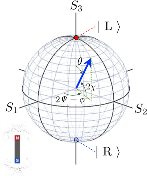
FIGURE 1. Bloch sphere for the polarisation states, described left and right circularly polarised states. The left (right) circularly polarised state is shown on the north (south) pole by the red (blue) colour at S₃ =1 (S₃= −1). The polarisation state is shown by the vector of spin angular momentum (blue arrow) at the position, described by the polar angle of θ and the azimuthal angle of ϕ. The dotted green line shows the projection of the spin angular momentum to the S₁-S₂ plane.

Thus, the corresponding coherent state with the spin state (θ, ϕ) is obtained as |α_Lα_R⟩ = |α_L⟩|α_R⟩, where.

$|{\alpha }_{\text{L}}\rangle ={\mathrm{e}}^{-\frac{|{\alpha }_{\text{L}}{|}^2}{2}}{\mathrm{e}}^{{\alpha }_{\text{L}}{\widehat{a}}_{\text{L}}^{†}}|0\rangle (60)$

$|{\alpha }_{\text{R}}\rangle ={\mathrm{e}}^{-\frac{|{\alpha }_{\text{R}}{|}^2}{2}}{\mathrm{e}}^{{\alpha }_{\text{R}}{\widehat{a}}_{\text{R}}^{†}}|0\rangle ,(61)$

for which we assign ${\alpha }_{\text{L}}=\sqrt{N}{\mathrm{e}}^{-i\frac{\varphi }{2}}\cos \left(\frac{\theta }{2}\right)$, ${\alpha }_{\text{R}}=\sqrt{N}{\mathrm{e}}^{+i\frac{\varphi }{2}}\sin \left(\frac{\theta }{2}\right)$. The complex electric field operator in the chiral representation is given by

$\widehat{\mathcal{E}}\left(z,t\right)=\sqrt{\frac{2\hslash \omega }{ϵV}}{\mathrm{e}}^{i\beta }\left({\widehat{a}}_{\text{L}}\widehat{\mathbf{l}}+{\widehat{a}}_{\text{R}}\widehat{\mathbf{r}}\right),(62)$

where $\widehat{\mathbf{l}}=(\widehat{\mathbf{x}}+i\widehat{\mathbf{y}})/\sqrt{2}$ and $\widehat{\mathbf{r}}=(\widehat{\mathbf{x}}-i\widehat{\mathbf{y}})/\sqrt{2}$ are complex unit vectors to describe directions of left and right polarisation states with phases. By applying this to the coherent state, we obtain the complex wavefunction in the chiral representation as

$\mathcal{E}\left(z,t\right)=\left(\begin{array}{c}\hfill {\mathcal{E}}_L\hfill \\ \hfill {\mathcal{E}}_R\hfill \end{array}\right)(63)$

$=E_0{\mathrm{e}}^{i\beta }\left(\begin{array}{c}\hfill {\mathrm{e}}^{-i\frac{\varphi }{2}}\cos \left(\frac{\theta }{2}\right)\hfill \\ \hfill {\mathrm{e}}^{+i\frac{\varphi }{2}}\sin \left(\frac{\theta }{2}\right)\hfill \end{array}\right)(64)$

$=E_0\mathrm{\Psi }\left(z,t\right)|\mathrm{B}\mathrm{l}\mathrm{o}\mathrm{c}\mathrm{h}\rangle .(65)$

By calculating the expectation values of spin components by the coherent state, we obtain

$\langle \widehat{\mathbf{S}}\rangle =\left(\begin{array}{c}\hfill \langle {\widehat{S}}_x\rangle \hfill \\ \hfill \langle {\widehat{S}}_y\rangle \hfill \\ \hfill \langle {\widehat{S}}_z\rangle \hfill \end{array}\right)(66)$

$=\hslash N\left(\begin{array}{c}\hfill \sin \theta \cos \varphi \hfill \\ \hfill \sin \theta \sin \varphi \hfill \\ \hfill \cos \theta \hfill \end{array}\right).(67)$

By realising the correspondences between angles,

$\theta =\frac{\pi }{2}-2\chi (68)$

$\varphi =2\mathit{\Psi }.(69)$

We realised

$⟨\widehat{\mathbf{S}}⟩=\hslash N\left(\begin{array}{c}\hfill \cos \left(2\chi \right)\cos \left(2\mathit{\Psi }\right)\hfill \\ \hfill \cos \left(2\chi \right)\sin \left(2\mathit{\Psi }\right)\hfill \\ \hfill \sin \left(2\chi \right)\hfill \end{array}\right)(70)$

$=\hslash N\left(\begin{array}{c}\hfill S_1\hfill \\ \hfill S_2\hfill \\ \hfill S_3\hfill \end{array}\right),(71)$

showing that the expectation values of the spin operators are essentially equivalent to the Stokes parameters. Thus, the Poincaré sphere is equivalent to the Bloch sphere.

It is also useful to define the spin operator to represent the magnitude of the spin,

${\widehat{S}}_0=\hslash \left({\widehat{a}}_{\text{L}}^{†}{\widehat{a}}_{\text{L}}+{\widehat{a}}_{\text{R}}^{†}{\widehat{a}}_{\text{R}}\right),(72)$

such that its expectation value is

$⟨{\widehat{S}}_0⟩=\hslash N.(73)$

This actually shows the order parameter of the coherent states. The onset of lasing is similar to the second order phase transition, which show the continuous increase of the macroscopic order parameter upon changing the control parameter such as temperature [48–55]. In the case for lasing, the control parameter is the pumping power, provided by injecting electrons and holes for a laser diode, or by optical populating of electrons to higher energy levels to realise a population inversion state. Above the lasing threshold, the macroscopic number of photons are degenerate to occupy the single mode, such that $⟨{\widehat{S}}_0⟩$ can posses a non-zero value, and $⟨{\widehat{S}}_0⟩$ increases gradually upon the increase of the pumping power.

The theory of the order parameter description of the phase transition was first developed for the theory of superconductivity, as the Ginzburg–Landau theory [48–55], for which the order parameter was the energy gap, |Δ|, and the U (1) gauge symmetry of the phase (e^iϕ) was broken. Therefore, the order parameter is described by a scalar.

In the case of lasing, two phases of the wave, such as (θ, ϕ) in chiral representation and (α, δ) in Jones representation, are fixed, and the order parameters are described by a vector, not by a scalar. This is why 3D vectorial representation using the Poincaré sphere is so useful [5,21,22].

The 3D description of the order parameter similar to the Poincaré sphere is not restricted to the photonic systems, and actually they are ubiquitously available for describing various order parameters. For example, magnetic Heisenberg model was used to describe the superfluid-solid phase transition for a liquid He [56]. Another example is the SO(5) (special orthogonal) theory, which was developed for describing antiferromagnetic-superconducting phase transition for high-critical-temperature superconducting cuprates [55,57].

These spin operators are previously known as Stokes operators [29–33,38,58,59], and their commutation relationships are

$\left[{\widehat{S}}_x,{\widehat{S}}_y\right]=2i\hslash {\widehat{S}}_z,\left[{\widehat{S}}_y,{\widehat{S}}_z\right]=2i\hslash {\widehat{S}}_x,\left[{\widehat{S}}_z,{\widehat{S}}_x\right]=2i\hslash {\widehat{S}}_y,(74)$

which are directly obtained by the commutation relationships of ${\widehat{a}}_{\sigma }^{†}$ and ${\widehat{a}}_{\sigma }$. The factor of 2 is unusual, because we have just 2 degrees of freedom, regardless of the spin 1 nature of a photon, which normally allow 3 states (1, 0, −1) along the principle quantisation axis [6–9]. This restriction is coming from the transverse nature of the ray of photons.

We also obtain

$\left[{\widehat{S}}_0,{\widehat{S}}_x\right]=\left[{\widehat{S}}_0,{\widehat{S}}_y\right]=\left[{\widehat{S}}_0,{\widehat{S}}_z\right]=0,(75)$

which are commutable, such that the magnitude can be a simultaneous eigenstate with the spin vector, $\widehat{\mathbf{S}}=\left({\widehat{S}}_x,{\widehat{S}}_y,{\widehat{S}}_z\right)$.

It is also intuitive to evaluate the quantum fluctuations [31–33] of the spin of photons, by calculating

$\widehat{\mathbf{S}}\cdot \widehat{\mathbf{S}}/{\hslash }^2=\left({\widehat{n}}_{\text{L}}+{\widehat{n}}_{\text{R}}\right)\left({\widehat{n}}_{\text{L}}+{\widehat{n}}_{\text{R}}+2\right)(76)$

$=\widehat{n}\left(\widehat{n}+2\right),(77)$

where $\widehat{n}={\widehat{n}}_{\text{L}}+{\widehat{n}}_{\text{R}}$ is the total number operator, and then we obtain the expectation value of the quantum-mechanical fluctuation as [31–33].

$\delta S=\sqrt{\frac{⟨\widehat{\mathbf{S}}\cdot \widehat{\mathbf{S}}⟩-{⟨{\widehat{S}}_0⟩}^2}{{⟨{\widehat{S}}_0⟩}^2}}(78)$

$=\sqrt{\frac{2}{N}},(79)$

Which means that the quantum-mechanical fluctuation decreases significantly upon increasing the order parameter. This is quite typical among other macroscopically quantum ordered systems [48,52–54].

3.2 Jones vector representation

Here, we will develop a similar description of spin of a photon, using Jones vector representation (Supplementary Material). Our starting point is

${\widehat{S}}_z=\left(-i\right)\hslash \left({\widehat{a}}_{\text{H}}^{†}{\widehat{a}}_{\text{V}}-{\widehat{a}}_{\text{V}}^{†}{\widehat{a}}_{\text{H}}\right),(80)$

$=\hslash \left(\begin{array}{cc}\hfill {\widehat{a}}_{\text{H}}^{†},\hfill & \hfill {\widehat{a}}_{\text{V}}^{†}\hfill \end{array}\right)\left(\begin{array}{cc}\hfill 0\hfill & \hfill -i\hfill \\ \hfill i\hfill & \hfill 0\hfill \end{array}\right)\left(\begin{array}{c}\hfill {\widehat{a}}_{\text{H}}\hfill \\ \hfill {\widehat{a}}_{\text{V}}\hfill \end{array}\right)(81)$

$=\hslash {\widehat{\mathit{\psi }}}_{\text{HV}}^{†}{\sigma }_2{\widehat{\mathit{\psi }}}_{\text{HV}},(82)$

where ${\widehat{\mathit{\psi }}}_{\text{HV}}^{†}=({\widehat{a}}_{\text{H}}^{†},{\widehat{a}}_{\text{V}}^{†})$ and ${\widehat{\mathit{\psi }}}_{\text{HV}}$ are the creation and annihilation operators in Jones vector representation. We also call this basis as the HV-basis. In the HV-basis, it is expected that the spin state is diagonalised along the horizontal and vertical directions, such that we can expect the spin operator along x as

${\widehat{S}}_x=\hslash {\widehat{\mathit{\psi }}}_{\text{HV}}^{†}{\sigma }_3{\widehat{\mathit{\psi }}}_{\text{HV}},(83)$

and consequently,

${\widehat{S}}_y=\hslash {\widehat{\mathit{\psi }}}_{\text{HV}}^{†}{\sigma }_1{\widehat{\mathit{\psi }}}_{\text{HV}},(84)$

for the y component, describing diagonal/anti-diagonal linear polarisation.

By taking the quantum-mechanical average over the coherent state, |α_H, α_V⟩, we obtain

$⟨\widehat{\mathbf{S}}⟩=\hslash N\left(\begin{array}{c}\hfill \cos \left(2\alpha \right)\hfill \\ \hfill \sin \left(2\alpha \right)\cos \delta \hfill \\ \hfill \sin \left(2\alpha \right)\sin \delta \hfill \end{array}\right),(85)$

which is shown on a Poincaré sphere of Figure 2.

FIGURE 2

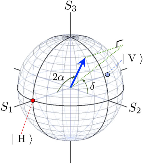
FIGURE 2. Poincaré sphere for the polarisation states, described by horizontally and vertically polarised states. For these basis states, the horizontal (vertical) linearly polarised state is shown on the north (south) pole by the red (blue) colour at S₁ = 1 (S₁ = −1). The polarisation state is shown by the vector of spin angular momentum (blue arrow) at the position, described by the polar angle of 2α and the azimuthal angle of δ. δ is known as the phase difference between horizontal and vertical modes and α is the auxiliary angle to split horizontal and vertical components. The dotted green line shows the projection of the spin angular momentum to the S₂-S₃ plane.

The expectation value must be independent on the choice of the fundamental basis. By comparing $⟨\widehat{\mathbf{S}}⟩$, obtained for both LR- and HV-bases, we obtain the identities,

$\tan \left(2\mathrm{\Psi }\right)=\tan \left(2\alpha \right)\cos \delta (86)$

$\sin \left(2\chi \right)=\sin \left(2\alpha \right)\sin \delta ,(87)$

for the transformations of angles. These are exactly the same ones as those obtained classically, by rotating the horizontal axis to the principal axis of the polarisation ellipse (Supplementary Material). Therefore, the rotation of the axes in the real space to change from (α, δ) to (χ, Ψ) is equivalent to transforming from Jones vector representation to chiral representation. The comparison between chiral and Jones representations are summarised in Table 1 for Poincaré sphere.

TABLE 1

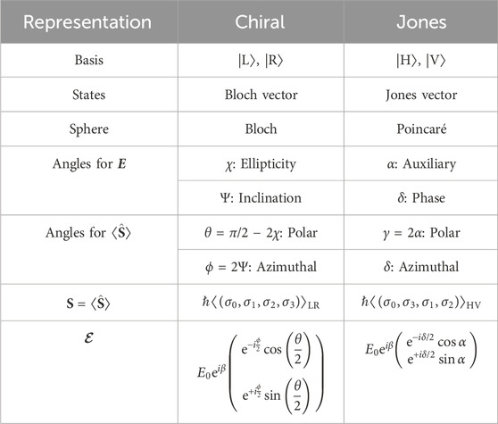
TABLE 1. Comparison between chiral and Jones representation for polarisation states.

The reason why the factor of 2 appeared in front of angles such as 2Ψ, 2χ, and 2α, is the quantum-mechanical average. By taking the complex conjugate and applying it to the original phase factor, we obtain this factor of 2, compared with the actual angle in the real space for E. This difference could be very important similar to geometrical Pancharatnam-Berry’s phase [61, 62], since the adiabatic rotation in Bloch/Poincaré sphere would not change the expectation value, but nevertheless, it can change the sign of the electric field, which leads the non-trivial interference [60].

3.3 Diagonal representation

We can also consider another representation, using diagonal |D⟩ and anti-diagonal |A⟩ basis states. In this basis, we will diagonalise the spin operator along y, and we obtain

${\widehat{S}}_x=\hslash {\widehat{\mathit{\psi }}}_{\text{DA}}^{†}{\sigma }_2{\widehat{\mathit{\psi }}}_{\text{DA}}(88)$

${\widehat{S}}_y=\hslash {\widehat{\mathit{\psi }}}_{\text{DA}}^{†}{\sigma }_3{\widehat{\mathit{\psi }}}_{\text{DA}}(89)$

${\widehat{S}}_z=\hslash {\widehat{\mathit{\psi }}}_{\text{DA}}^{†}{\sigma }_1{\widehat{\mathit{\psi }}}_{\text{DA}},(90)$

where ${\widehat{\mathit{\psi }}}_{\text{DA}}^{†}=({\widehat{a}}_{\text{D}}^{†},{\widehat{a}}_{\text{A}}^{†})$ and ${\widehat{\mathit{\psi }}}_{\text{DA}}$ are the creation and the annihilation operator in the diagonal representation. For this DA-representation, the coherent state and the average of the spin operators are best described by the polar angle θ′ measured from the S₂ axis and the azimuthal angle ϕ′ measured from the S₃ axis (Figure 3). The expectation value is given by

$⟨\widehat{\mathbf{S}}⟩=\hslash N\left(\begin{array}{c}\hfill 1\hfill \\ \hfill \sin {\theta }^{\prime }\sin {\varphi }^{\prime }\hfill \\ \hfill \cos {\theta }^{\prime }\hfill \\ \hfill \sin {\theta }^{\prime }\cos {\varphi }^{\prime }\hfill \end{array}\right).(91)$

FIGURE 3

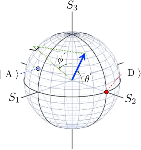
FIGURE 3. Poincaré sphere for the polarisation states, described by diagonally and anti-diagonally polarised states. The diagonal (anti-diagonal) linearly polarised state is shown on the north (south) pole by the red (blue) colour at S₂ = 1 (S₂ = −1). The polarisation state is shown by the vector of spin angular momentum (blue arrow) at the position, described by the polar angle of θ′ and the azimuthal angle of ϕ′. The dotted green line shows the projection of the spin angular momentum to the S₃-S₁ plane.

As far as we are aware, this representation is barely used.

3.4 Unitary transformation from HV- to LR-bases

Now, we realise the Jones vector treatments of the polarisation states are fully consistent with the quantum-mechanical treatment in SU(2). Here, we will double check this equivalence by transforming the Jones vector state to the corresponding representation in chiral state, which is made by the unitary transformation

$\left(\begin{array}{c}\hfill |\mathrm{H}\rangle \hfill \\ \hfill |\mathrm{V}\rangle \hfill \end{array}\right)=\frac{{\mathrm{e}}^{i\gamma }}{\sqrt{2}}\left(\begin{array}{cc}\hfill 1\hfill & \hfill 1\hfill \\ \hfill -i\hfill & \hfill i\hfill \end{array}\right)\left(\begin{array}{c}\hfill |\mathrm{L}\rangle \hfill \\ \hfill |\mathrm{R}\rangle \hfill \end{array}\right),(92)$

where γ is the uncertainty of the global U (1) phase.

The original Jones vector is prepared as.

$|\alpha ,\delta \rangle ={\mathrm{e}}^{i\beta }\left(\begin{array}{c}\hfill \cos \alpha \hfill \\ \hfill \sin \alpha {\mathrm{e}}^{i\delta }\hfill \end{array}\right)(93)$

$={\mathrm{e}}^{i\beta }\cos \alpha |\mathrm{H}\rangle +{\mathrm{e}}^{i\beta }\sin \alpha {\mathrm{e}}^{i\delta }|\mathrm{V}\rangle ,(94)$

and after the unitary transformation, we obtain in the form of

$|\alpha ,\delta \rangle =C_{\text{L}}|\mathrm{L}\rangle +C_{\text{R}}|\mathrm{R}\rangle =|\theta ,\varphi \rangle .(95)$

Therefore, we need to determine C_L and C_R, which are.

$C_{\text{L}}={\mathrm{e}}^{i\left(\beta +\gamma \right)}\frac{\cos \alpha -i{\mathrm{e}}^{i\delta }\sin \alpha }{\sqrt{2}}(96)$

$C_{\text{R}}={\mathrm{e}}^{i\left(\beta +\gamma \right)}\frac{\cos \alpha +i{\mathrm{e}}^{i\delta }\sin \alpha }{\sqrt{2}}.(97)$

We still need to express these as a function of (θ, ϕ).

To this aid, we assume the expectation values of $⟨\widehat{\mathbf{S}}⟩$ are independent on the choice of the basis states.

The ratio of the coefficient becomes

$\frac{C_{\text{R}}}{C_{\text{L}}}=\tan \left(\frac{\theta }{2}\right){\mathrm{e}}^{i\varphi }.(98)$

In addition, we can confirm that the wavefunction is normalised

$|C_{\text{L}}{|}^2+|C_{\text{R}}{|}^2=1.(99)$

These equations for 2 complex values of C_L and C_R correspond to 3 equations for real values. Therefore, we cannot determine the global phase degree of freedom, e^iγ.

Assuming $C_{\text{L}}=l\in \mathfrak{R}$, we obtain $C_{\text{R}}=l\tan \left(\theta /2\right){\mathrm{e}}^{i\varphi }$. Inserting this into the normalisation condition, we obtain $l=\pm \cos \left(\theta /2\right)$. Thus, we obtain 2 states,

$\left(\begin{array}{c}\hfill C_{\text{L}}\hfill \\ \hfill C_{\text{R}}\hfill \end{array}\right)=\pm \left(\begin{array}{c}\hfill \cos \left(\frac{\theta }{2}\right)\hfill \\ \hfill {\mathrm{e}}^{i\varphi }\sin \left(\frac{\theta }{2}\right)\hfill \end{array}\right),(100)$

which yield the same expectation value but the overall sign is opposite each other. This phase is different from the global phase, and this is coming from the two-fold coverage of SU(2) as SU(2)/SO(3) ≈ Z₂ = {−1, 1}, according to the mathematical theory for isomorphism [64, 65, 66? ]. We know that the wavefunction of the polarisation state is the spinor representation of the complex electric field. Therefore, the factor of −1 means that the change between $({\mathcal{E}}_x,{\mathcal{E}}_y)$ and $(-{\mathcal{E}}_x,-{\mathcal{E}}_y)$, which cannot change the polarisation state, but the phase is observable in the interference experiments [60–62]. We can express these states together, by shifting the global phase, while keeping the relative phase, as

$\left(\begin{array}{c}\hfill C_{\text{L}}\hfill \\ \hfill C_{\text{R}}\hfill \end{array}\right)=\left(\begin{array}{c}\hfill {\mathrm{e}}^{-i\varphi /2}\cos \left(\frac{\theta }{2}\right)\hfill \\ \hfill {\mathrm{e}}^{+i\varphi /2}\sin \left(\frac{\theta }{2}\right)\hfill \end{array}\right),(101)$

which is indeed the Bloch vector. Here, we should consider the range of ϕ should be (0, 4π) to account for the change of the sign. Thus, the Jones vector is equivalent to the Bloch vector.

It is less obvious of this sign change in the above-defined Jones vector, if we describe the phase dependence as e^iδ. This could be improved by shifting the global phase with the amount of e^iδ/2, and then Jones vector can be rewritten as

$|\mathrm{J}\mathrm{o}\mathrm{n}\mathrm{e}\mathrm{s}\rangle ={\mathrm{e}}^{i\beta }\left(\begin{array}{c}\hfill {\mathrm{e}}^{-i\delta /2}\cos \left(\gamma /2\right)\hfill \\ \hfill {\mathrm{e}}^{i\delta /2}\sin \left(\gamma /2\right)\hfill \end{array}\right),(102)$

where γ = 2α is the azimuthal angle measured from S₁ on the Poincaré sphere (Figure 2). In this spinor representation, it is clear that the state will change the sign after 1 rotation on the Poincaré sphere, irrespective to whether the adiabatic rotation is the azimuthal rotation along the equator or the polar rotation along the meridian. This is exactly the same form of the Bloch state in chiral state, such that the change of basis from LR to HV simply corresponds to change from (θ, ϕ) to (γ, δ) in polar coordinates. This corresponds to the cyclic exchange of Pauli matrices from (σ₁, σ₂, σ₃) to (σ₃, σ₁, σ₂) (Table 2).

TABLE 2

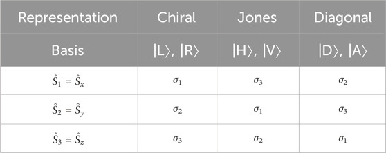
TABLE 2. Summary of spin operators for each representation.

3.5 Spin rotation by an SU(2) group theory

Now, we understand the spin state of a photon is described by an SU(2) group theory [6–9]. By using a standard Lie algebra, using Pauli matrices, we can obtain the many-body spin operators for the coherent monochromatic ray for photons, in a more elegant way. The general rotation operator [6–9] along the direction $\widehat{\mathbf{n}}$ with the amount of δϕ is defined as

$\widehat{\mathcal{D}}\left(\widehat{\mathbf{n}},\delta \varphi \right)=\exp \left(-i\mathit{\sigma }\cdot \widehat{\mathbf{n}}\left(\frac{\delta \varphi }{2}\right)\right),(103)$

where $|\widehat{\widehat{\mathrm{n}}}|=1$ and σ = (σ₁, σ₂, σ₃). We have chosen the direction of rotation in a standard mathematical way. Specifically, the positive rotation along z is equivalent to the left-hand rotation (anti-clock-wise) rotation in xy-plane, seen from the top of the z-axis, which is equivalent to see from the observer in the detector side. By expanding the exponential and using the formulas, $\left\{{\sigma }_i,{\sigma }_j\right\}=2{\delta }_{ij}\mathbf{1}$, and $\left[{\sigma }_i,{\sigma }_j\right]=2i{ϵ}_{\mathit{ijk}}{\sigma }_k$, we obtain [6–9].

$\widehat{\mathcal{D}}\left(\widehat{\mathbf{n}},\delta \varphi \right)=\mathbf{1}\cos \left(\frac{\delta \varphi }{2}\right)-i\mathit{\sigma }\cdot \widehat{\mathbf{n}}\sin \left(\frac{\delta \varphi }{2}\right).(104)$

In particular, we describe the rotation around x, y, and z, axes as ${\widehat{\mathcal{D}}}_1(\delta \varphi )={\widehat{\mathcal{D}}}_x(\delta \varphi )=\widehat{\mathcal{D}}(\widehat{\mathbf{x}},\delta \varphi )$, ${\widehat{\mathcal{D}}}_2(\delta \varphi )={\widehat{\mathcal{D}}}_y(\delta \varphi )=\widehat{\mathcal{D}}(\widehat{\mathbf{y}},\delta \varphi )$, and ${\widehat{\mathcal{D}}}_3(\delta \varphi )={\widehat{\mathcal{D}}}_z(\delta \varphi )=\widehat{\mathcal{D}}(\widehat{\mathbf{z}},\delta \varphi )$, for simplicity.

Previously, as outlined above, the spin operator along the direction of propagation $({\widehat{S}}_z)$ was obtained by using the Poynting vector and considerations of angular momentum [4,5,11–18]. Then, we can obtain the spin operator along x, ${\widehat{S}}_x$, by rotating ${\widehat{S}}_z$ with the amount of π/2 along y, and therefore,

${\widehat{S}}_x={\widehat{\mathcal{D}}}_y\left(\frac{\pi }{2}\right){\widehat{S}}_z{\widehat{\mathcal{D}}}_y^{†}\left(\frac{\pi }{2}\right)(105)$

$={\widehat{\mathcal{D}}}_y\left(\frac{\pi }{2}\right){\mathit{\psi }}_{\text{LR}}^{†}\hslash {\sigma }_3{\mathit{\psi }}_{\text{LR}}{\widehat{\mathcal{D}}}_y^{†}\left(\frac{\pi }{2}\right)(106)$

$={\mathit{\psi }}_{\text{LR}}^{†}{\widehat{\mathcal{D}}}_y\left(\frac{\pi }{2}\right)\hslash {\sigma }_3{\widehat{\mathcal{D}}}_y^{†}\left(\frac{\pi }{2}\right){\mathit{\psi }}_{\text{LR}}(107)$

$=\hslash {\mathit{\psi }}_{\text{LR}}^{†}{\sigma }_1{\mathit{\psi }}_{\text{LR}}.(108)$

Similarly, we obtain ${\widehat{S}}_y$ from ${\widehat{S}}_z$ by rotating along x with the amount of −π/2 as

${\widehat{S}}_y={\widehat{\mathcal{D}}}_x\left(-\frac{\pi }{2}\right){\widehat{S}}_z{\widehat{\mathcal{D}}}_x^{†}\left(-\frac{\pi }{2}\right)(109)$

$={\widehat{\mathcal{D}}}_x\left(-\frac{\pi }{2}\right){\mathit{\psi }}_{\text{LR}}^{†}\hslash {\sigma }_3{\mathit{\psi }}_{\text{LR}}{\widehat{\mathcal{D}}}_x^{†}\left(-\frac{\pi }{2}\right)(110)$

$={\mathit{\psi }}_{\text{LR}}^{†}{\widehat{\mathcal{D}}}_x\left(-\frac{\pi }{2}\right)\hslash {\sigma }_3{\widehat{\mathcal{D}}}_x^{†}\left(-\frac{\pi }{2}\right){\mathit{\psi }}_{\text{LR}}(111)$

$=\hslash {\mathit{\psi }}_{\text{LR}}^{†}{\sigma }_2{\mathit{\psi }}_{\text{LR}}.(112)$

Alternatively, we can also rotate 2π/3 along $(\mathrm{1,1,1})/\sqrt{3}$ direction, for cyclic permutation of axes. The rotation operator becomes

$\widehat{\mathcal{D}}\left(\frac{\left(\mathrm{1,1,1}\right)}{\sqrt{3}},\frac{2\pi }{3}\right)=\frac{1}{2}-\frac{i}{2}\left({\sigma }_1+{\sigma }_2+{\sigma }_3\right),(113)$

which yields

$\widehat{\mathcal{D}}\left(\frac{\left(\mathrm{1,1,1}\right)}{\sqrt{3}},\frac{2\pi }{3}\right){\sigma }_3\widehat{\mathcal{D}}{\left(\frac{\left(\mathrm{1,1,1}\right)}{\sqrt{3}},\frac{2\pi }{3}\right)}^{†}={\sigma }_1.(114)$

Therefore, we successfully obtain ${\widehat{S}}_x$, and the opposite rotation yield ${\widehat{S}}_y$.

For the expressions using the HV-basis, we can use a unitary transformation

$\left(\begin{array}{c}\hfill {\widehat{a}}_{\text{H}}^{†}\hfill \\ \hfill {\widehat{a}}_{\text{V}}^{†}\hfill \end{array}\right)=\frac{1}{\sqrt{2}}\left(\begin{array}{cc}\hfill 1\hfill & \hfill 1\hfill \\ \hfill -i\hfill & \hfill i\hfill \end{array}\right)\left(\begin{array}{c}\hfill {\widehat{a}}_{\text{L}}^{†}\hfill \\ \hfill {\widehat{a}}_{\text{R}}^{†}\hfill \end{array}\right),(115)$

and its conjugate

$\left(\begin{array}{c}\hfill {\widehat{a}}_{\text{H}}\hfill \\ \hfill {\widehat{a}}_{\text{V}}\hfill \end{array}\right)=\frac{1}{\sqrt{2}}\left(\begin{array}{cc}\hfill 1\hfill & \hfill 1\hfill \\ \hfill i\hfill & \hfill -i\hfill \end{array}\right)\left(\begin{array}{c}\hfill {\widehat{a}}_{\text{L}}\hfill \\ \hfill {\widehat{a}}_{\text{R}}\hfill \end{array}\right).(116)$

We can, of course, come back to LR-basis from HV-basis by the inverse unitary transformation. The transfer to the DA-basis is also straightforward by using the unitary transformation

$\left(\begin{array}{c}\hfill {\widehat{a}}_{\text{D}}^{†}\hfill \\ \hfill {\widehat{a}}_{\text{A}}^{†}\hfill \end{array}\right)=\frac{1}{\sqrt{2}}\left(\begin{array}{cc}\hfill 1\hfill & \hfill 1\hfill \\ \hfill 1\hfill & \hfill -1\hfill \end{array}\right)\left(\begin{array}{c}\hfill {\widehat{a}}_{\text{H}}^{†}\hfill \\ \hfill {\widehat{a}}_{\text{V}}^{†}\hfill \end{array}\right),(117)$

and its conjugate

$\left(\begin{array}{c}\hfill {\widehat{a}}_{\text{D}}\hfill \\ \hfill {\widehat{a}}_{\text{A}}\hfill \end{array}\right)=\frac{1}{\sqrt{2}}\left(\begin{array}{cc}\hfill 1\hfill & \hfill 1\hfill \\ \hfill 1\hfill & \hfill -1\hfill \end{array}\right)\left(\begin{array}{c}\hfill {\widehat{a}}_{\text{H}}\hfill \\ \hfill {\widehat{a}}_{\text{V}}\hfill \end{array}\right).(118)$

The summary of the assignments of Pauli matrices to spin operator components for each representation is given by Table 2.

3.6 Rotation in real space

Here, we consider the rotation in real space rather than Hilbert space for spin. We define the rotation operators for the amount of the rotation of δϕ along x, y, and z-axes as ${\mathcal{R}}_x(\delta \varphi )$, ${\mathcal{R}}_y(\delta \varphi )$, ${\mathcal{R}}_z(\delta \varphi )$, respectively. These are rotations in a SO(3) (Special Orthogonal) group theory. By applying 2 successive rotations along y and x,

${\mathcal{R}}_x\left(\frac{\pi }{2}\right){\mathcal{R}}_y\left(\frac{\pi }{2}\right)\widehat{\mathbf{x}}=\widehat{\mathbf{y}}(119)$

${\mathcal{R}}_x\left(\frac{\pi }{2}\right){\mathcal{R}}_y\left(\frac{\pi }{2}\right)\widehat{\mathbf{y}}=\widehat{\mathbf{z}}(120)$

${\mathcal{R}}_x\left(\frac{\pi }{2}\right){\mathcal{R}}_y\left(\frac{\pi }{2}\right)\widehat{\mathbf{z}}=\widehat{\mathbf{x}}.(121)$

We can perform cyclic exchange of axes from (x, y, z) to (y, z, x) as

${\mathcal{R}}_x\left(\frac{\pi }{2}\right){\mathcal{R}}_y\left(\frac{\pi }{2}\right)=\left(\begin{array}{ccc}\hfill 0\hfill & \hfill 0\hfill & \hfill 1\hfill \\ \hfill 1\hfill & \hfill 0\hfill & \hfill 0\hfill \\ \hfill 0\hfill & \hfill 1\hfill & \hfill 0\hfill \end{array}\right).(122)$

If we apply this rotations to $\widehat{\mathbf{E}}$, we obtain the corresponding electric field operator after 2 successive rotations as

$\begin{array}{ccc}\hfill {\widehat{\mathbf{E}}}^{\prime \prime }=& \hfill & \frac{E_0}{2}\left({\widehat{a}}_{\text{H}}{\mathrm{e}}^{i{\beta }^{\prime \prime }}+{\widehat{a}}_{\text{H}}^{†}{\mathrm{e}}^{-i{\beta }^{\prime \prime }}\right)\widehat{\mathbf{y}}\hfill \\ \hfill & \hfill & +\frac{E_0}{2}\left({\widehat{a}}_{\text{V}}{\mathrm{e}}^{i{\beta }^{\prime \prime }}+{\widehat{a}}_{\text{V}}^{†}{\mathrm{e}}^{-i{\beta }^{\prime \prime }}\right)\widehat{\mathbf{z}},\hfill \end{array}(123)$

where β′′ = kx − ωt + δ_x.

Then, by applying the same argument using the Poynting vector, we obtain the momentum operator and the total angular momentum after the rotations as

${\widehat{\mathbf{P}}}^{\prime \prime }=\hslash k_{n_0}\left({\widehat{n}}_{\text{H}}+{\widehat{n}}_{\text{V}}+1\right)\widehat{\mathbf{x}},(124)$

${\widehat{\mathbf{J}}}_z^{\prime \prime }={\widehat{\mathbf{S}}}_z^{\prime \prime }={\widehat{S}}_z\widehat{\mathbf{x}},(125)$

where

${\widehat{S}}_z=\hslash \left({\widehat{n}}_{\text{L}}-{\widehat{n}}_{\text{R}}\right).(126)$

This means that the spatial rotations simply change the direction of propagation, but the polarisation state is not changed. We could also confirm that the polarisation state has not been changed by the opposite rotation for the left cyclic exchange from (x, y, z) to (z, y, x) by using the SO(3) rotation

${\mathcal{R}}_x\left(-\frac{\pi }{2}\right){\mathcal{R}}_y\left(-\frac{\pi }{2}\right)=\left(\begin{array}{ccc}\hfill 0\hfill & \hfill 1\hfill & \hfill 0\hfill \\ \hfill 0\hfill & \hfill 0\hfill & \hfill 1\hfill \\ \hfill 1\hfill & \hfill 0\hfill & \hfill 0\hfill \end{array}\right).(127)$

Of course, the polarisation should not depend on the choice of the spatial coordinate, since the polarisation is a measure to evaluate the relative phase between orthogonal polarisation states, which cannot be changed by the rotation for the direction of propagation, which is responsible to the overall phase of both polarisation states, equally.

${\widehat{S}}_z$ and thus $S_3=⟨{\widehat{S}}_z⟩$ are inherently linked to the direction of the propagation. Therefore, it is natural to regard ${\widehat{S}}_z$ as the helicity operator [63],

${\widehat{h}}_z=\hslash \left({\widehat{n}}_{\text{L}}-{\widehat{n}}_{\text{R}}\right).(128)$

The helicity is usually defined as the projection of the spin onto the direction of the propagation, and in fact ${\widehat{h}}_z=\widehat{\mathbf{S}}\cdot \widehat{\mathbf{z}}$, for the light propagating along z. We have defined the polarisation states from the electro-magnetic field oscillations seen from the detector side, such that the helicity operator becomes

$\widehat{h}=\hslash \left({\widehat{n}}_{\text{L}}-{\widehat{n}}_{\text{R}}\right),(129)$

independent on the direction of propagation.

We could also define our spin operators as.

${\widehat{S}}_1=\hslash {\widehat{\mathit{\psi }}}_{\text{LR}}^{†}{\sigma }_1{\widehat{\mathit{\psi }}}_{\text{LR}}(130)$

${\widehat{S}}_2=\hslash {\widehat{\mathit{\psi }}}_{\text{LR}}^{†}{\sigma }_2{\widehat{\mathit{\psi }}}_{\text{LR}}(131)$

${\widehat{S}}_3=\hslash {\widehat{\mathit{\psi }}}_{\text{LR}}^{†}{\sigma }_3{\widehat{\mathit{\psi }}}_{\text{LR}},(132)$

to emphasise the direct relevance to the Stokes parameters as $⟨{\widehat{S}}_i⟩=S_i$ for ^∀i = 0, 1, 2, 3. Even in this notation, we still need to clarify the direction of the propagation, otherwise the spin state and the polarisation state cannot be properly specified. The way to define the rotation, whether the phase front is rotating to the left (anti-clock-wise) or to the right (clock-wise), depends crucially on the definition of the direction of the propagation. The definition of the rotation is also important and we have assumed the polarisation is seen from the observer (detector) in this paper. We have discussed, by assuming the direction of the propagation is mostly along z, and defined spin operators, accordingly. Here, we have shown that the polarisation state, thus defined, should not depend on the direction of the propagation, such that the spin operators and associated expectation values as Stokes parameters should not depend on the choice of the coordinate. The direction of the propagation of photons naturally set the quantisation axis for their inherent spin states, as confirmed by the spatial integration of the outer product between r and the Poynting vector. We confirmed ${\widehat{S}}_z={\widehat{S}}_3={\widehat{h}}_z=\widehat{h}$ is always aligned to the direction of propagation.

One might attempt to align the direction of spin operators to a specific axis in an arbitrary chosen coordinate. However, in this case, the artificially fixed spin operator is not always aligned to the direction of the propagation, such that ${\widehat{S}}_z$ may not be aligned to the direction of the propagation. In such a coordinate, it is very difficult to discuss the polarisation state, even if it is possible.

The choice of the coordinate should be arbitrary, according to Einstein’s theory of relativity. The quantisation axis of the spin operator for describing the amount of the circular polarised state is naturally aligned to the direction of the propagation. We do not know why the spin quantisation axis is locked to the direction of the propagation, but if we accept this as a principle, we could construct spin operators for other components, just by following a standard quantum-mechanical prescription and an SU(2) group theory.

4 Applications

As applications of our formalism, we consider several typical optical components to control the polarisation states [1,2,5,20–22,28,45–47,64–72]. Practically, this is nothing new compared with well-established Jones matrix formulation, but the purpose of this consideration is to establish a fundamental basis to justify the calculation of polarisation states using Jones matrices based on a many-body quantum physics and an SU(2) group theory.

4.1 Phase-shifter

4.1.1 Phase-shifter in the HV-basis

A phase-shifter is an optical component, which control the phase of δ by injecting a coherent laser beam with a specific polarisation state into it and changing the polarisation state of the output beam [5,21,22]. It is also called as a retarder, but we prefer to call it as a phase-shifter, because we can allow both retardation and advancement of the phase, just by changing the angle of the optical component. It is also called as a wave-plate. It is best-described by the HV-basis, so that we will discuss in the HV-basis, first and then, transform the formulas to those in the LR-basis.

The working principle of the phase-shifter is quite simple. It is based on a birefringence of a transparent single crystal such as quartz, LiNbO₃, and other transparent single crystals [5,21,22]. In these birefringent materials, the values of the refractive index depend on the direction of the propagation against their crystal axis. The axis for the large refractive index (n_s) is called as a slow axis, and the axis for the small refractive index (n_f) is called as a fast axis, because the phase velocity of the slow axis (v_s) is slower than the phase velocity of the fast axis (v_f). We abbreviate slow axis as SA and fast axis as FA. This induces the polarisation dependent phase-shift, through the factor of e^ikx.

Specifically, first, we consider the retarder configuration, (Figures 4A, B), which means that the SA is aligned horizontally, and we expect the phase delay given by δ_fs = k₀ (n_f − n_s)d < 0, where k₀ = 2π/λ is the wavenumber in the vacuum, λ is the wavelength in the vacuum, and d is the thickness of the wave plate. The wavenumbers for SA and FA are given by k_s = k₀n_s and k_f = k₀n_f, respectively. We also define the average wavenumber as $\bar{k}=(k_{\text{s}}+k_{\text{f}})/2$.

FIGURE 4

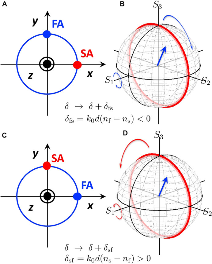
FIGURE 4. Phase-shifter and its impact on the polarisation state. (A) Retarder configuration. Slow axis (SA) is aligned horizontally. (B) Clock-wise rotation of the polarisation state by a retarder. The polarisation state shown by the vector (blue arrow) is the spin angular momentum, which is rotated along the clock-wise direction (blue curves) by the retarder. (C) Phase-shifter (phase-advancement) configuration. Fast axis (FA) is aligned horizontally. (D) Anti-clock-wise rotation of the polarisation state by a phase-shifter. The polarisation state shown by the vector (blue arrow) is the spin angular momentum, which is rotated along the anti-clock-wise direction (red curves) by the phase-shifter. This rotation is described by Δ_HV(δ_sf) or Δ_LR (δ_sf).

The many-body operator to describe this change is given by the following phase-shifter operator

${\widehat{\mathrm{\Delta }}}_{\text{HV}}\left({\delta }_{fs}\right)={\mathrm{e}}^{i{k}_{\text{s}}d}\frac{{\mathrm{e}}^{i\beta }}{\sqrt{N}}{\widehat{a}}_{\text{H}}\widehat{\mathbf{x}}+{\mathrm{e}}^{i{k}_{\text{f}}d}\frac{{\mathrm{e}}^{i\beta }}{\sqrt{N}}{\widehat{a}}_{\text{V}}\widehat{\mathbf{y}}.(133)$

By applying this to the coherent state, we obtain

$\begin{array}{ccc}\hfill & \hfill & {\widehat{\mathrm{\Delta }}}_{\text{HV}}\left({\delta }_{fs}\right)|{\alpha }_{\text{H}},{\alpha }_{\text{V}}\rangle \hfill \\ \hfill & \hfill & ={\mathrm{e}}^{i\beta }{\mathrm{e}}^{i\bar{k}d}\left(\begin{array}{cc}\hfill {\mathrm{e}}^{-i\frac{{\delta }_{\text{fs}}}{2}}\hfill & \hfill 0\hfill \\ \hfill 0\hfill & \hfill {\mathrm{e}}^{+i\frac{{\delta }_{\text{fs}}}{2}}\hfill \end{array}\right)\left(\begin{array}{c}\hfill {\mathrm{e}}^{-i\frac{\delta }{2}}\cos \alpha \hfill \\ \hfill {\mathrm{e}}^{+i\frac{\delta }{2}}\sin \alpha \hfill \end{array}\right)|{\alpha }_{\text{H}},{\alpha }_{\text{V}}\rangle \hfill \end{array}(134)$

which means that ${\widehat{\mathrm{\Delta }}}_{\text{HV}}$ does not change the number of photons and just affect the polarisation state. If we multiply the ket vector of the coherent state, ⟨α_H, α_V|, from the left, we obtain the expectation value of the phase-shifter operator in the retarder configuration as.

$\begin{array}{ccc}\hfill & \hfill & \langle {\alpha }_{\text{H}},{\alpha }_{\text{V}}|{\widehat{\mathrm{\Delta }}}_{\text{HV}}\left({\delta }_{fs}\right)|{\alpha }_{\text{H}},{\alpha }_{\text{V}}\rangle \hfill \\ \hfill & \hfill & ={\mathrm{e}}^{i\beta }{\mathrm{e}}^{i\bar{k}d}\left(\begin{array}{cc}\hfill {\mathrm{e}}^{-i\frac{{\delta }_{\text{fs}}}{2}}\hfill & \hfill 0\hfill \\ \hfill 0\hfill & \hfill {\mathrm{e}}^{+i\frac{{\delta }_{\text{fs}}}{2}}\hfill \end{array}\right)\left(\begin{array}{c}\hfill {\mathrm{e}}^{-i\frac{\delta }{2}}\cos \alpha \hfill \\ \hfill {\mathrm{e}}^{+i\frac{\delta }{2}}\sin \alpha \hfill \end{array}\right)\hfill \end{array}(135)$

$={\mathrm{\Delta }}_{\text{HV}}\left({\delta }_{\text{fs}}\right)|\mathrm{J}\mathrm{o}\mathrm{n}\mathrm{e}\mathrm{s}\rangle ,(136)$

where we have defined the Jones matrix for the phase-shifter as

${\mathrm{\Delta }}_{\text{HV}}\left({\delta }_{\text{fs}}\right)={\mathrm{e}}^{i\beta }{\mathrm{e}}^{i\bar{k}d}\left(\begin{array}{cc}\hfill {\mathrm{e}}^{-i\frac{{\delta }_{\text{fs}}}{2}}\hfill & \hfill 0\hfill \\ \hfill 0\hfill & \hfill {\mathrm{e}}^{+i\frac{{\delta }_{\text{fs}}}{2}}\hfill \end{array}\right),(137)$

Therefore, we can calculate the polarisation state of the ray after the propagation of the retarder by using the Jones matrix [1,2,5,21,22,28]. In the Poincaré sphere, this corresponds to rotate S along S₁ with the amount of δ_fs (Figure 4B). This corresponds to the clock-wise rotation, since δ_fs < 0.

Next, we consider the phase-shifter configuration, which corresponds to increase the phase by aligning FA horizontally (Figures 4C, D). In this case, the phase-shifter operator is given by

${\widehat{\mathrm{\Delta }}}_{\text{HV}}\left({\delta }_{sf}\right)={\mathrm{e}}^{i{k}_{\text{f}}d}\frac{{\mathrm{e}}^{i\beta }}{\sqrt{N}}{\widehat{a}}_{\text{H}}\widehat{\mathbf{x}}+{\mathrm{e}}^{i{k}_{\text{s}}d}\frac{{\mathrm{e}}^{i\beta }}{\sqrt{N}}{\widehat{a}}_{\text{V}}\widehat{\mathbf{y}},(138)$

which just corresponds to exchanging SA and FA, so that the above formulas are valid just by replacing δ_fs to δ_sf = k₀ (n_s − n_f)d > 0. Therefore, we obtain the Jones matrix

${\mathrm{\Delta }}_{\text{HV}}\left({\delta }_{\text{sf}}\right)={\mathrm{e}}^{i\beta }{\mathrm{e}}^{i\bar{k}d}\left(\begin{array}{cc}\hfill {\mathrm{e}}^{-i\frac{{\delta }_{\text{sf}}}{2}}\hfill & \hfill 0\hfill \\ \hfill 0\hfill & \hfill {\mathrm{e}}^{+i\frac{{\delta }_{\text{sf}}}{2}}\hfill \end{array}\right).(139)$

In this case, the operation of the phase-shifter is simply the phase-shift of δ → δ + δ_sf. Alternatively, we can regard the retarder as a special case of the phase-shifter with opposite rotation. The phase-shifter configuration (horizontal FA) is our preferable configuration to think about the rotation on the Poincaré sphere, since we can consider positive rotation, but of course, we can use both configurations depending on the applications.

It is now clear that the phase-shifter operator will change the polarisation state of the coherent state as an out put beam.

$|\mathrm{o}\mathrm{u}\mathrm{t}\mathrm{p}\mathrm{u}\mathrm{t}\rangle ={\widehat{\mathrm{\Delta }}}_{\text{HV}}\left({\delta }_{sf}\right)|\mathrm{i}\mathrm{n}\mathrm{p}\mathrm{u}\mathrm{t}\rangle$

$={\mathrm{e}}^{i\beta }{\mathrm{e}}^{i\bar{k}d}\left(\begin{array}{c}\hfill {\mathrm{e}}^{-i\frac{\delta +{\delta }_{\text{sf}}}{2}}\cos \alpha \hfill \\ \hfill {\mathrm{e}}^{+i\frac{\delta +{\delta }_{\text{sf}}}{2}}\sin \alpha \hfill \end{array}\right)|\mathrm{i}\mathrm{n}\mathrm{p}\mathrm{u}\mathrm{t}\rangle ,(140)$

where the input beam is |input⟩ = |α_H, α_V⟩. Therefore, the phase-shifter changes the relative phase to describe the spin states, while the coherency of the monochromatic ray of photons, described by coherent states is preserved. This aspect can be more clearly confirmed by calculating the average quantum-mechanical expectation value of the spin of photons, using the output state,

$⟨\mathrm{o}\mathrm{u}\mathrm{t}\mathrm{p}\mathrm{u}\mathrm{t}|\widehat{\mathbf{S}}|\mathrm{o}\mathrm{u}\mathrm{t}\mathrm{p}\mathrm{u}\mathrm{t}⟩=\hslash N\left(\begin{array}{c}\hfill \cos \left(\gamma \right)\hfill \\ \hfill \sin \left(\gamma \right)\cos \left(\delta +{\delta }_{\text{sf}}\right)\hfill \\ \hfill \sin \left(\gamma \right)\sin \left(\delta +{\delta }_{\text{sf}}\right)\hfill \end{array}\right).(141)$

Thus, the spin is rotated along S₁ with the amount of δ_sf by the phase-shifter (Figure 4D).

4.1.2 Phase-shifter as a rotator in SU(2) hilbert space

Aside from the overall phase factor, the phase shifter can be described by a rotation in SU(2) Hilbert space for spin of a photon. The phase-shifter corresponds to the rotation along S₁, such that the phase-shifter matrix in the HV-basis is described as.

${\mathcal{D}}_1^{\text{HV}}\left({\delta }_{\text{sf}}\right)=\exp \left(-\frac{i{\sigma }_3{\delta }_{\text{sf}}}{2}\right)(142)$

$=\mathbf{1}\cos \left(\frac{{\delta }_{\text{sf}}}{2}\right)-i{\sigma }_3\sin \left(\frac{{\delta }_{\text{sf}}}{2}\right)(143)$

$=\left(\begin{array}{cc}\hfill \exp \left(-i\frac{{\delta }_{\text{sf}}}{2}\right)\hfill & \hfill 0\hfill \\ \hfill 0\hfill & \hfill \exp \left(+i\frac{{\delta }_{\text{sf}}}{2}\right)\hfill \end{array}\right).(144)$

Combined with the overall phase factor, coming from the average global phase of the orbital wavefunction, we obtain.

${\mathrm{\Delta }}_{\text{HV}}\left({\delta }_{\text{sf}}\right)={\mathrm{e}}^{i\beta }{\mathrm{e}}^{i\bar{k}d}{\mathcal{D}}_1^{\text{HV}}\left({\delta }_{\text{sf}}\right)(145)$

$={\mathrm{e}}^{i\beta }{\mathrm{e}}^{i\bar{k}d}\left(\begin{array}{cc}\hfill {\mathrm{e}}^{-i\frac{{\delta }_{\text{sf}}}{2}}\hfill & \hfill 0\hfill \\ \hfill 0\hfill & \hfill {\mathrm{e}}^{+i\frac{{\delta }_{\text{sf}}}{2}}\hfill \end{array}\right),(146)$

which is exactly the same as that obtained previously. Therefore, the SU(2) group theory is a powerful method to consider the impact of the phase-shifter on the Poincaré sphere.

The retarder configuration (horizontal SA) is obviously corresponds to the opposite rotation (Figures 4B, D), whose operator form is obtained by the change of sign, due to δ_fs = −δ_sf.

4.1.3 Phase-shifter in the LR-basis

Here, we obtain the phase-shifter operator in chiral LR-basis. In the LR-basis, the rotation along S₁ is described by σ₁ (Table 2). Therefore, the Jones matrix for the phase-shifter in the LR-basis is

${\mathrm{\Delta }}_{\text{LR}}\left({\delta }_{\text{sf}}\right)={\mathrm{e}}^{i\beta }{\mathrm{e}}^{i\bar{k}d}{\mathcal{D}}_1^{\text{LR}}\left({\delta }_{\text{sf}}\right)(147)$

$={\mathrm{e}}^{i\beta }{\mathrm{e}}^{i\bar{k}d}\exp \left(-\frac{i{\sigma }_1{\delta }_{\text{sf}}}{2}\right)(148)$

$={\mathrm{e}}^{i\beta }{\mathrm{e}}^{i\bar{k}d}\left(\mathbf{1}\cos \left(\frac{{\delta }_{\text{sf}}}{2}\right)-i{\sigma }_1\sin \left(\frac{{\delta }_{\text{sf}}}{2}\right)\right)$

$={\mathrm{e}}^{i\beta }{\mathrm{e}}^{i\bar{k}d}\left(\begin{array}{cc}\hfill \cos \left(\frac{{\delta }_{\text{sf}}}{2}\right)\hfill & \hfill -i\sin \left(\frac{{\delta }_{\text{sf}}}{2}\right)\hfill \\ \hfill -i\sin \left(\frac{{\delta }_{\text{sf}}}{2}\right)\hfill & \hfill \cos \left(\frac{{\delta }_{\text{sf}}}{2}\right)\hfill \end{array}\right).(149)$

4.1.4 Unitary operation

LR-basis can be transferred to the HV-basis by a unitary transformation,

$U_{\text{HV}}=\frac{1}{\sqrt{2}}\left(\begin{array}{cc}\hfill 1\hfill & \hfill 1\hfill \\ \hfill i\hfill & \hfill -i\hfill \end{array}\right),(150)$

and vice versa by the inverse

$U_{\text{HV}}^{†}=\frac{1}{\sqrt{2}}\left(\begin{array}{cc}\hfill 1\hfill & \hfill -i\hfill \\ \hfill 1\hfill & \hfill i\hfill \end{array}\right).(151)$

Therefore, any operator in the HV-basis, O_HV, can be transferred to that in the LR-basis, O_HV, by the unitary transformation

$O_{\text{LR}}=U_{\text{HV}}^{-1}{O}_{\text{HV}}{U}_{\text{HV}},(152)$

which means that the state in the LR-basis is first transformed to the HV-basis by U_HV, operated in the HV-space by O_HV, and finally brought back to the LR-basis by $U_{\text{HV}}^{-1}$. We confirm this operation for the above obtained phase-shifter. In order to confirm, we directly calculated.

${\mathrm{\Delta }}_{\text{LR}}\left({\delta }_{\text{sf}}\right)=U_{\text{HV}}^{-1}{\mathrm{\Delta }}_{\text{HV}}{U}_{\text{HV}}(153)$

$=\frac{1}{\sqrt{2}}\left(\begin{array}{cc}\hfill 1\hfill & \hfill -i\hfill \\ \hfill 1\hfill & \hfill i\hfill \end{array}\right){\mathrm{e}}^{i\beta }{\mathrm{e}}^{i\bar{k}d}\left(\begin{array}{cc}\hfill {\mathrm{e}}^{-i\frac{{\delta }_{\text{sf}}}{2}}\hfill & \hfill 0\hfill \\ \hfill 0\hfill & \hfill {\mathrm{e}}^{+i\frac{{\delta }_{\text{sf}}}{2}}\hfill \end{array}\right)\frac{1}{\sqrt{2}}\left(\begin{array}{cc}\hfill 1\hfill & \hfill 1\hfill \\ \hfill i\hfill & \hfill -i\hfill \end{array}\right)$

$={\mathrm{e}}^{i\beta }{\mathrm{e}}^{i\bar{k}d}\left(\begin{array}{cc}\hfill \cos \left(\frac{{\delta }_{\text{sf}}}{2}\right)\hfill & \hfill -i\sin \left(\frac{{\delta }_{\text{sf}}}{2}\right)\hfill \\ \hfill -i\sin \left(\frac{{\delta }_{\text{sf}}}{2}\right)\hfill & \hfill \cos \left(\frac{{\delta }_{\text{sf}}}{2}\right)\hfill \end{array}\right),(154)$

which is indeed successfully transferred. Therefore, the unitary transformation is useful to change the basis states.

4.2 Rotator

4.2.1 Rotator in the LR-basis

The idea of the phase-shifter is to utilise the orbital degree of the wavefunction to tune the relative phase between two orthogonal polarisation states by using a polarisation dependent material for changing the polarisation state. The directional dependence of the refractive indexes was the key ingredient for enabling the phase-shift.

Here, we show very similar formulation is applicable to a rotator. In a rotator, the chiral dependence of the refractive indexes are used to control the relative phase between left and right circular polarised states. Consequently, it is straightforward to construct an operator in the chiral LR-basis.

The key ingredient for enabling the chirality control is the refractive index dependence on chirality in materials like quartz and liquid crystal [24,73]. One of the most important application of the control of chirality of photons is the use for a Liquid-Crystal-Display (LCD). By applying voltage to the transparent capacitor, organic molecule sandwiched between two parallel electrodes of capacitors can align towards the electric field, which changes the refractive index to switch the pixel on and off. Left-handed quartz and right-handed quartz are also known to be optically active materials due to their chiral atomic arrangements of the network of silicon-oxide bonds [24]. A material with a chiral dependence should have such atomic or molecular structures, which are optically active dependent on the polarisation state of the chiral S₃ component.

We assume a rotator made of an optically active material with the thickness of d and the refractive indexes for left and right circular-polarised states are n_L and n_R, whose wavenumbers are k_L = k₀n_L and k_R = k₀n_R, respectively. Then, the many-body rotator operator is given by

${\widehat{\mathcal{R}}}_{\text{LR}}\left(\mathrm{\Delta }\varphi \right)={\mathrm{e}}^{i{k}_{\text{L}}d}\frac{{\mathrm{e}}^{i\beta }}{\sqrt{N}}{\widehat{a}}_{\text{L}}\widehat{\mathbf{l}}+{\mathrm{e}}^{i{k}_{\text{R}}d}\frac{{\mathrm{e}}^{i\beta }}{\sqrt{N}}{\widehat{a}}_{\text{R}}\widehat{\mathbf{r}},(155)$

where Δϕ is the amount of the rotation, which we shall obtain next. By applying this to the coherent state, we obtain the output state

$\begin{array}{ccc}\hfill & \hfill & |\mathrm{o}\mathrm{u}\mathrm{t}\mathrm{p}\mathrm{u}\mathrm{t}\rangle ={\widehat{\mathcal{R}}}_{\text{LR}}\left(\mathrm{\Delta }\varphi \right)|{\alpha }_{\text{L}},{\alpha }_{\text{R}}\rangle \hfill \\ \hfill & \hfill & ={\mathrm{e}}^{i\beta }{\mathrm{e}}^{i\bar{k}d}\left(\begin{array}{cc}\hfill {\mathrm{e}}^{-i\frac{\mathrm{\Delta }\varphi }{2}}\hfill & \hfill 0\hfill \\ \hfill 0\hfill & \hfill {\mathrm{e}}^{+i\frac{\mathrm{\Delta }\varphi }{2}}\hfill \end{array}\right)\left(\begin{array}{c}\hfill {\mathrm{e}}^{-i\frac{\varphi }{2}}\cos \left(\theta /2\right)\hfill \\ \hfill {\mathrm{e}}^{+i\frac{\varphi }{2}}\sin \left(\theta /2\right)\hfill \end{array}\right)|{\alpha }_{\text{L}},{\alpha }_{\text{R}}\rangle ,\hfill \end{array}(156)$

where Δϕ = 2ρd is the rotation angle of the azimuthal direction on the Poincaré sphere, ΔΨ = ρd is the rotation angle of the inclination angle for the electric field of the principal axis in the polarisation ellipse, and ρ = (k_R − k_L)d/2 = π(n_R − n_L)/λ. By applying ⟨α_L, α_R| from the left, we obtain.

$\begin{array}{ccc}\hfill & \hfill & \langle {\alpha }_{\text{L}},{\alpha }_{\text{R}}|{\widehat{\mathcal{R}}}_{\text{LR}}\left(\mathrm{\Delta }\varphi \right)|{\alpha }_{\text{L}},{\alpha }_{\text{R}}\rangle \hfill \\ \hfill & \hfill & ={\mathrm{e}}^{i\beta }{\mathrm{e}}^{i\bar{k}d}\left(\begin{array}{cc}\hfill {\mathrm{e}}^{-i\frac{\mathrm{\Delta }\varphi }{2}}\hfill & \hfill 0\hfill \\ \hfill 0\hfill & \hfill {\mathrm{e}}^{+i\frac{\mathrm{\Delta }\varphi }{2}}\hfill \end{array}\right)\left(\begin{array}{c}\hfill {\mathrm{e}}^{-i\frac{\varphi }{2}}\cos \left(\theta /2\right)\hfill \\ \hfill {\mathrm{e}}^{+i\frac{\varphi }{2}}\sin \left(\theta /2\right)\hfill \end{array}\right)\hfill \end{array}(157)$

$={\mathcal{R}}_{\text{LR}}\left(\mathrm{\Delta }\varphi \right)|\mathrm{B}\mathrm{l}\mathrm{o}\mathrm{c}\mathrm{h}\rangle ,(158)$

where we have obtained the Jones matrix for a rotator as

${\mathcal{R}}_{\text{LR}}\left(\mathrm{\Delta }\varphi \right)={\mathrm{e}}^{i\beta }{\mathrm{e}}^{i\bar{k}d}\left(\begin{array}{cc}\hfill {\mathrm{e}}^{-i\frac{\mathrm{\Delta }\varphi }{2}}\hfill & \hfill 0\hfill \\ \hfill 0\hfill & \hfill {\mathrm{e}}^{+i\frac{\mathrm{\Delta }\varphi }{2}}\hfill \end{array}\right).(159)$

After the propagation in the rotator, the output beam state becomes.

$|\mathrm{o}\mathrm{u}\mathrm{t}\mathrm{p}\mathrm{u}\mathrm{t}\rangle ={\widehat{\mathcal{R}}}_{\text{LR}}\left(\mathrm{\Delta }\varphi \right)|\mathrm{i}\mathrm{n}\mathrm{p}\mathrm{u}\mathrm{t}\rangle (160)$

$={\mathrm{e}}^{i\beta }{\mathrm{e}}^{i\bar{k}d}\left(\begin{array}{c}\hfill {\mathrm{e}}^{-i\frac{\varphi +\mathrm{\Delta }\varphi }{2}}\cos \left(\theta /2\right)\hfill \\ \hfill {\mathrm{e}}^{+i\frac{\varphi +\mathrm{\Delta }\varphi }{2}}\sin \left(\theta /2\right)\hfill \end{array}\right)|\mathrm{i}\mathrm{n}\mathrm{p}\mathrm{u}\mathrm{t}\rangle .(161)$

By taking the quantum-mechanical expectation values of the output state, we obtain

$⟨\mathrm{o}\mathrm{u}\mathrm{t}\mathrm{p}\mathrm{u}\mathrm{t}|\widehat{\mathbf{S}}|\mathrm{o}\mathrm{u}\mathrm{t}\mathrm{p}\mathrm{u}\mathrm{t}⟩=\hslash N\left(\begin{array}{c}\hfill \sin \theta \cos \left(\varphi +\mathrm{\Delta }\varphi \right)\hfill \\ \hfill \sin \theta \sin \left(\varphi +\mathrm{\Delta }\varphi \right)\hfill \\ \hfill \cos \theta \hfill \end{array}\right),(162)$

which means that the rotator successfully rotate the polarisation state as the expectation value of the spin vector on the Poincaré sphere with the amount of Δϕ along the S₃ axis (Figure 5).

FIGURE 5

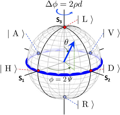
FIGURE 5. Rotator and its impact on the polarisation state. The polarisation state shown by the vector (blue arrow) is the spin angular momentum, which is rotated along the clock-wise direction (blue curve) by the rotator for the amount of Δϕ.

4.2.2 Rotator as a rotator in SU(2) hilbert space

We understand the chiral phase-control corresponds to the rotation around S₃ on the Poincaré sphere. ${\widehat{S}}_3$ corresponds to σ₃ in the chiral LR-basis (Table 2). Then, we can construct a rotator based on an SU(2) group theory by

${\mathcal{D}}_3^{\text{LR}}\left(\mathrm{\Delta }\varphi \right)=\exp \left(-\frac{i{\sigma }_3\mathrm{\Delta }\varphi }{2}\right)(163)$

$=\mathbf{1}\cos \left(\frac{\mathrm{\Delta }\varphi }{2}\right)-i{\sigma }_3\sin \left(\frac{\mathrm{\Delta }\varphi }{2}\right)(164)$

$=\left(\begin{array}{cc}\hfill \exp \left(-i\frac{\mathrm{\Delta }\varphi }{2}\right)\hfill & \hfill 0\hfill \\ \hfill 0\hfill & \hfill \exp \left(+i\frac{\mathrm{\Delta }\varphi }{2}\right)\hfill \end{array}\right).(165)$

With the inclusion of the overall phase for the global orbital contribution, the Jones matrix becomes

${\mathcal{R}}_{\text{LR}}\left(\mathrm{\Delta }\varphi \right)={\mathrm{e}}^{i\beta }{\mathrm{e}}^{i\bar{k}d}{\mathcal{D}}_3^{\text{LR}}\left(\mathrm{\Delta }\varphi \right),(166)$

which is in agreement with the previous many-body operator based calculation.

4.2.3 Rotator in the HV-basis

It is also straightforward to obtain the rotator in the HV-basis by an SU(2) group theory. ${\widehat{S}}_3$ corresponds to σ₂ in the HV-basis (Table 2), such that, we can construct a rotator by the operator

${\mathcal{D}}_3^{\text{HV}}\left(\mathrm{\Delta }\varphi \right)=\exp \left(-\frac{i{\sigma }_2\mathrm{\Delta }\varphi }{2}\right)(167)$

$=\mathbf{1}\cos \left(\frac{\mathrm{\Delta }\varphi }{2}\right)-i{\sigma }_2\sin \left(\frac{\mathrm{\Delta }\varphi }{2}\right)(168)$

$=\left(\begin{array}{cc}\hfill 1\hfill & \hfill 0\hfill \\ \hfill 0\hfill & \hfill 1\hfill \end{array}\right)\cos \left(\frac{\mathrm{\Delta }\varphi }{2}\right)+\left(\begin{array}{cc}\hfill 0\hfill & \hfill -1\hfill \\ \hfill 1\hfill & \hfill 0\hfill \end{array}\right)\sin \left(\frac{\mathrm{\Delta }\varphi }{2}\right)(169)$

$=\left(\begin{array}{cc}\hfill \cos \left(\frac{\mathrm{\Delta }\varphi }{2}\right)\hfill & \hfill -\sin \left(\frac{\mathrm{\Delta }\varphi }{2}\right)\hfill \\ \hfill \sin \left(\frac{\mathrm{\Delta }\varphi }{2}\right)\hfill & \hfill \cos \left(\frac{\mathrm{\Delta }\varphi }{2}\right)\hfill \end{array}\right)(170)$

$=\left(\begin{array}{cc}\hfill \cos \left(\mathrm{\Delta }\mathit{\Psi }\right)\hfill & \hfill -\sin \left(\mathrm{\Delta }\mathit{\Psi }\right)\hfill \\ \hfill \sin \left(\mathrm{\Delta }\mathit{\Psi }\right)\hfill & \hfill \cos \left(\mathrm{\Delta }\mathit{\Psi }\right)\hfill \end{array}\right).(171)$

With the phase factor, Jones matrix for a rotator in the HV-basis becomes

${\mathcal{R}}_{\text{HV}}\left(\mathrm{\Delta }\varphi \right)={\mathrm{e}}^{i\beta }{\mathrm{e}}^{i\bar{k}d}{\mathcal{D}}_3^{\text{HV}}\left(\mathrm{\Delta }\varphi \right).(172)$

We realise that this corresponds to a standard SO(3) rotation

$R_z\left(\mathrm{\Delta }\mathit{\Psi }\right)=\left(\begin{array}{cc}\hfill \cos \left(\mathrm{\Delta }\mathit{\Psi }\right)\hfill & \hfill -\sin \left(\mathrm{\Delta }\mathit{\Psi }\right)\hfill \\ \hfill \sin \left(\mathrm{\Delta }\mathit{\Psi }\right)\hfill & \hfill \cos \left(\mathrm{\Delta }\mathit{\Psi }\right)\hfill \end{array}\right)(173)$

of $\mathcal{E}$ along z. In fact, the complex electric field is simply rotated upon the operation of the rotator as

$\left(\begin{array}{c}\hfill {\mathcal{E}}_x^{\prime }\hfill \\ \hfill {\mathcal{E}}_y^{\prime }\hfill \end{array}\right)={\mathrm{e}}^{i\beta }{\mathrm{e}}^{i\bar{k}d}{R}_z\left(\mathrm{\Delta }\mathit{\Psi }\right)\left(\begin{array}{c}\hfill {\mathcal{E}}_x\hfill \\ \hfill {\mathcal{E}}_y\hfill \end{array}\right),(174)$

including the global phase factor, where ${\mathcal{E}}^{\prime }=({\mathcal{E}}_x^{\prime },{\mathcal{E}}_y^{\prime })$ is the complex output electric field. Therefore, the impact of a rotator as an passive optical component is equivalent to a physical anti-clockwise rotation of the electric field, which is also identical to the rotation of (x, y)-axes along z in the opposite direction (clock-wise). During this rotation, the angle of χ is preserved, such that the shape of the polarisation ellipse is not affected. The rotation of the principal axis in the real space of ΔΨ corresponds to the rotation of $⟨\widehat{\mathbf{S}}⟩$ with the amount of Δϕ = 2ΔΨ. The factor of 2 is again coming from the quantum-mechanical expectation value. It is very useful to remember that the rotation in real space affects twice the rotation of $⟨\widehat{\mathbf{S}}⟩$ on the Poincaré sphere. We should always be aware of this difference between real space and Poincaré sphere.

It is also interesting to note that the physical rotation of a rotator cannot change the operation. This can be checked simply by calculating

${\mathcal{D}}_3^{†}\left(\mathrm{\Delta }{\varphi }^{\prime }\right){\mathcal{D}}_3\left(\mathrm{\Delta }\varphi \right){\mathcal{D}}_3\left(\mathrm{\Delta }{\varphi }^{\prime }\right)={\mathcal{D}}_3\left(\mathrm{\Delta }\varphi \right),(175)$

which is valid for both LR- and HV-bases. Therefore, the physical rotation of a rotator will not change the polarisation state of the output beam.

4.2.4 Unitary transformation

We have obtained Jones matrix for a rotator both in LR- and HV-bases. As is expected for other quantum systems, these descriptions must be identical and transferable to one from the other by unitary transformation. In order to transfer from ${\mathcal{R}}_{\text{HV}}(\mathrm{\Delta }\varphi )$ to ${\mathcal{R}}_{\text{LR}}(\mathrm{\Delta }\varphi )$, we use U_HV and we confirmed

${\mathcal{R}}_{\text{LR}}\left(\mathrm{\Delta }\varphi \right)=U_{\text{HV}}^{-1}{\mathcal{R}}_{\text{HV}}\left(\mathrm{\Delta }\varphi \right)U_{\text{HV}}(176)$

$=\frac{{\mathrm{e}}^{i\beta }{\mathrm{e}}^{i\bar{k}d}}{2}\left(\begin{array}{cc}\hfill 1\hfill & \hfill -i\hfill \\ \hfill 1\hfill & \hfill i\hfill \end{array}\right)\left(\begin{array}{cc}\hfill \cos \left(\frac{\mathrm{\Delta }\varphi }{2}\right)\hfill & \hfill -\sin \left(\frac{\mathrm{\Delta }\varphi }{2}\right)\hfill \\ \hfill \sin \left(\frac{\mathrm{\Delta }\varphi }{2}\right)\hfill & \hfill \cos \left(\frac{\mathrm{\Delta }\varphi }{2}\right)\hfill \end{array}\right)\left(\begin{array}{cc}\hfill 1\hfill & \hfill 1\hfill \\ \hfill i\hfill & \hfill -i\hfill \end{array}\right)$

$={\mathrm{e}}^{i\beta }{\mathrm{e}}^{i\bar{k}d}\left(\begin{array}{cc}\hfill \exp \left(-i\frac{\mathrm{\Delta }\varphi }{2}\right)\hfill & \hfill 0\hfill \\ \hfill 0\hfill & \hfill \exp \left(+i\frac{\mathrm{\Delta }\varphi }{2}\right)\hfill \end{array}\right),(177)$

which is in agreement with our result.

For the opposite transformation, from ${\mathcal{R}}_{\text{LR}}(\mathrm{\Delta }\varphi )$ to ${\mathcal{R}}_{\text{HV}}(\mathrm{\Delta }\varphi )$, we use $U_{\text{LR}}=U_{\text{HV}}^{-1}$ and we confirmed

${\mathcal{R}}_{\text{HV}}\left(\mathrm{\Delta }\varphi \right)=U_{\text{LR}}^{-1}{\mathcal{R}}_{\text{LR}}{U}_{\text{LR}}(178)$

$=\frac{{\mathrm{e}}^{i\beta }{\mathrm{e}}^{i\bar{k}d}}{2}\left(\begin{array}{cc}\hfill 1\hfill & \hfill 1\hfill \\ \hfill i\hfill & \hfill -i\hfill \end{array}\right)\left(\begin{array}{cc}\hfill {\mathrm{e}}^{-i\frac{\mathrm{\Delta }\varphi }{2}}\hfill & \hfill 0\hfill \\ \hfill 0\hfill & \hfill {\mathrm{e}}^{+i\frac{\mathrm{\Delta }\varphi }{2}}\hfill \end{array}\right)\left(\begin{array}{cc}\hfill 1\hfill & \hfill -i\hfill \\ \hfill 1\hfill & \hfill i\hfill \end{array}\right)$

$={\mathrm{e}}^{i\beta }{\mathrm{e}}^{i\bar{k}d}\left(\begin{array}{cc}\hfill \cos \left(\frac{\mathrm{\Delta }\varphi }{2}\right)\hfill & \hfill -\sin \left(\frac{\mathrm{\Delta }\varphi }{2}\right)\hfill \\ \hfill \sin \left(\frac{\mathrm{\Delta }\varphi }{2}\right)\hfill & \hfill \cos \left(\frac{\mathrm{\Delta }\varphi }{2}\right)\hfill \end{array}\right).(179)$

Therefore, a standard unitary transformation and its inverse are applicable to the polarisation operators.

4.3 Rotated phase-shifter

4.3.1 Rotated phase-shifter in the HV-basis

As an application of the phase-shifter and the rotator, discussed above, we consider a rotated phase-shifter with the amount of ΔΨ, whose FA was originally aligned horizontally (Figure 6).

FIGURE 6

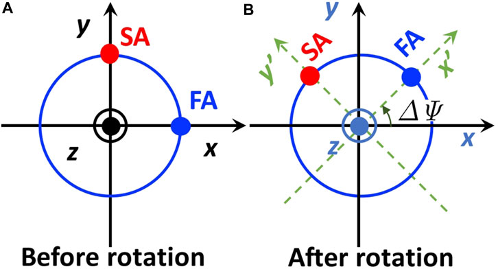
FIGURE 6. Rotated phase-shifter. (A) Phase-shifter arrangement before rotation. The fast axis (FA) is horizontally aligned, while the slow axis (SA) is vertical. (B) After rotation of ΔΨ in the anti-clock-wise direction (left rotation), seen from the top of the z-axis. The x-y axes are rotated to be x′-y′ axes upon the rotation (green dotted lines).

It is straightforward to obtain the Jones matrix of the rotated phase-shifter, by following the several steps. First, we consider the rotation of the coordinate from (x, y) to (x′, y′)-axes, which is described by a standard rotation around z-axis as

$\left(\begin{array}{c}\hfill x^{\prime }\hfill \\ \hfill y^{\prime }\hfill \end{array}\right)=R_z\left(\mathrm{\Delta }\mathit{\Psi }\right)\left(\begin{array}{c}\hfill x\hfill \\ \hfill y\hfill \end{array}\right).(180)$

The rotation of the coordinate is equivalent to the rotation of the physical vector (in this case, complex electric field) in the opposite direction

$\left(\begin{array}{c}\hfill {\mathcal{E}}_x^{\prime }\hfill \\ \hfill {\mathcal{E}}_y^{\prime }\hfill \end{array}\right)=R_z\left(-\mathrm{\Delta }\mathit{\Psi }\right)\left(\begin{array}{c}\hfill {\mathcal{E}}_x\hfill \\ \hfill {\mathcal{E}}_y\hfill \end{array}\right).(181)$

Next, we will apply the phase-shifter operation in the rotated frame as

$\left(\begin{array}{c}\hfill {\mathcal{E}}_x^{\prime \prime }\hfill \\ \hfill {\mathcal{E}}_y^{\prime \prime }\hfill \end{array}\right)={\mathrm{\Delta }}_{\text{HV}}\left({\delta }_{\text{sf}}\right)R_z\left(-\mathrm{\Delta }\mathit{\Psi }\right)\left(\begin{array}{c}\hfill {\mathcal{E}}_x\hfill \\ \hfill {\mathcal{E}}_y\hfill \end{array}\right).(182)$

Finally, we will bring back to the original frame as

$\left(\begin{array}{c}\hfill {\mathcal{E}}_x^{‴}\hfill \\ \hfill {\mathcal{E}}_y^{‴}\hfill \end{array}\right)=R_z\left(\mathrm{\Delta }\mathit{\Psi }\right){\mathrm{\Delta }}_{\text{HV}}\left({\delta }_{\text{sf}}\right)R_z\left(-\mathrm{\Delta }\mathit{\Psi }\right)\left(\begin{array}{c}\hfill {\mathcal{E}}_x\hfill \\ \hfill {\mathcal{E}}_y\hfill \end{array}\right).(183)$

Then, we obtain the Jones matrix for the rotated phase-shifter as

$\begin{array}{ccc}\hfill & \hfill & {\mathrm{\Delta }}_{\text{HV}}\left(\mathrm{\Delta }\varphi ,{\delta }_{\text{sf}}\right)\hfill \\ \hfill & \hfill & ={\mathrm{e}}^{i\beta }{\mathrm{e}}^{i\bar{k}d}\left(\cos \left(\frac{{\delta }_{\text{sf}}}{2}\right)\mathbf{1}-i\sin \left(\frac{{\delta }_{\text{sf}}}{2}\right)\left(\begin{array}{cc}\hfill \cos \left(\mathrm{\Delta }\varphi \right)\hfill & \hfill \sin \left(\mathrm{\Delta }\varphi \right)\hfill \\ \hfill \sin \left(\mathrm{\Delta }\varphi \right)\hfill & \hfill -\cos \left(\mathrm{\Delta }\varphi \right)\hfill \end{array}\right)\right),\hfill \end{array}(184)$

where Δϕ = 2ΔΨ as usual.

It is especially important at Δϕ = π/2 (ΔΨ = π/4), which corresponds to the case of 45° rotated phase-shifter, given by

${\mathrm{\Delta }}_{\text{HV}}\left(\mathrm{\Delta }\varphi =\pi /2,{\delta }_{\text{sf}}\right)={\mathrm{e}}^{i\beta }{\mathrm{e}}^{i\bar{k}d}\left(\cos \left(\frac{{\delta }_{\text{sf}}}{2}\right)\mathbf{1}-i\sin \left(\frac{{\delta }_{\text{sf}}}{2}\right){\sigma }_1\right),$

$={\mathrm{e}}^{i\beta }{\mathrm{e}}^{i\bar{k}d}\exp \left(-\frac{i{\sigma }_1{\delta }_{\text{sf}}}{2}\right)(185)$

$={\mathrm{e}}^{i\beta }{\mathrm{e}}^{i\bar{k}d}{\mathcal{D}}_2^{\text{HV}}\left({\delta }_{\text{sf}}\right).(186)$

because the rotation along S₂ corresponds to σ₁ in the HV-basis (Table 2). This is useful to use, when we want to convert from LR-states to HV-states and vice versa (Figure 7).

FIGURE 7

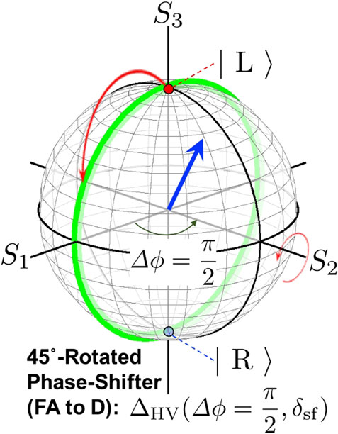
FIGURE 7. 45° rotated phase-shifter. The operation corresponds to the rotation of polarisation state along S₂, which is described by Δ_HV(Δϕ = π/2, δ_sf). The polarisation state shown by the vector (blue arrow) is the spin angular momentum, which is rotated along the anti-clock-wise direction (red curves) by the phase-shifter. If the initial polarisation states are left (red point on the north pole) and right (blue point on the south pole) circularly polarised states, they are rotated along the longitude (green curve).

If we use this 45°-rotated phase-shifter to the coherent state, described by diagonal basis (Figure 3), the spin expectation value of the output state,

$|\mathrm{o}\mathrm{u}\mathrm{t}\mathrm{p}\mathrm{u}\mathrm{t}\rangle ={\mathrm{\Delta }}_{\text{HV}}\left(\mathrm{\Delta }\varphi =\pi /2,{\delta }_{\text{sf}}\right)|\mathrm{i}\mathrm{n}\mathrm{p}\mathrm{u}\mathrm{t}\rangle ,(187)$

is rotated δ_sf along S₂, and therefore, we obtain

$⟨\mathrm{o}\mathrm{u}\mathrm{t}\mathrm{p}\mathrm{u}\mathrm{t}|\widehat{\mathbf{S}}|\mathrm{o}\mathrm{u}\mathrm{t}\mathrm{p}\mathrm{u}\mathrm{t}⟩=\hslash N\left(\begin{array}{c}\hfill \sin {\theta }^{\prime }\sin \left({\varphi }^{\prime }+{\delta }_{\text{sf}}\right)\hfill \\ \hfill \cos {\theta }^{\prime }\hfill \\ \hfill \sin {\theta }^{\prime }\cos \left({\varphi }^{\prime }+{\delta }_{\text{sf}}\right)\hfill \end{array}\right).(188)$

4.3.2 Rotated phase-shifter in the LR-basis

Similarly, it is straightforward to obtain the general rotated phase-shifter in the LR-basis as.

${\mathrm{\Delta }}_{\text{LR}}\left(\mathrm{\Delta }\varphi ,{\delta }_{\text{sf}}\right)={\mathcal{R}}_{\text{LR}}\left(\mathrm{\Delta }\varphi \right){\mathrm{\Delta }}_{\text{LR}}\left({\delta }_{\text{sf}}\right){\mathcal{R}}_{\text{LR}}\left(-\mathrm{\Delta }\varphi \right)$

$={\mathrm{e}}^{i\beta }{\mathrm{e}}^{i\bar{k}d}\left(\begin{array}{cc}\hfill \cos \left(\frac{{\delta }_{\text{sf}}}{2}\right)\hfill & \hfill -i{\mathrm{e}}^{-i\mathrm{\Delta }\varphi }\sin \left(\frac{{\delta }_{\text{sf}}}{2}\right)\hfill \\ \hfill -i{\mathrm{e}}^{+i\mathrm{\Delta }\varphi }\sin \left(\frac{{\delta }_{\text{sf}}}{2}\right)\hfill & \hfill \cos \left(\frac{{\delta }_{\text{sf}}}{2}\right)\hfill \end{array}\right),(189)$

which Δϕ = π/2

${\mathrm{\Delta }}_{\text{LR}}\left(\mathrm{\Delta }\varphi =\pi /2,{\delta }_{\text{sf}}\right)={\mathrm{e}}^{i\beta }{\mathrm{e}}^{i\bar{k}d}\left(\begin{array}{cc}\hfill \cos \left(\frac{{\delta }_{\text{sf}}}{2}\right)\hfill & \hfill -\sin \left(\frac{{\delta }_{\text{sf}}}{2}\right)\hfill \\ \hfill \sin \left(\frac{{\delta }_{\text{sf}}}{2}\right)\hfill & \hfill \cos \left(\frac{{\delta }_{\text{sf}}}{2}\right)\hfill \end{array}\right),$

$={\mathrm{e}}^{i\beta }{\mathrm{e}}^{i\bar{k}d}\exp \left(-\frac{i{\sigma }_2{\delta }_{\text{sf}}}{2}\right)(190)$

$={\mathrm{e}}^{i\beta }{\mathrm{e}}^{i\bar{k}d}{\mathcal{D}}_2^{\text{LR}}\left({\delta }_{\text{sf}}\right),(191)$

because the rotation along S₂ corresponds to σ₂ in the LR-basis (Table 2).

4.3.3 Rotated phase-shifter in SU(2) hilbert space

We can easily obtain above formulas in consideration of a quantum-mechanical SU(2) theory. The phase-shifter is described by a rotator of an SU(2) group with the rotation axis in the S₁-S₂ plane. If we rotate the phase-shifter with the amount of ΔΨ in the real space (Figure 6B), the rotation axis on the Poincaré sphere corresponds to the direction n = (cos (Δϕ), sin (Δϕ), 0), where Δϕ = 2ΔΨ. Therefore, the rotated phase-shifter corresponds to the rotator of spin states in SU(2) Hilbert space along n with the amount of Δϕ. Away from the global phase factor, this rotation is described by the operator, for the HV-basis, as

$\begin{array}{c}{\mathcal{D}}_{xy}^{\text{HV}}\left({\delta }_{\text{sf}}\right)=\mathbf{1}\cos \left(\frac{{\delta }_{\text{sf}}}{2}\right)-i{\sigma }_3\cos \left(\mathrm{\Delta }\varphi \right)\sin \left(\frac{{\delta }_{\text{sf}}}{2}\right)\hfill \\ -i{\sigma }_1\sin \left(\mathrm{\Delta }\varphi \right)\sin \left(\frac{{\delta }_{\text{sf}}}{2}\right)\hfill \end{array}$

$=\cos \left(\frac{{\delta }_{\text{sf}}}{2}\right)\mathbf{1}-i\sin \left(\frac{{\delta }_{\text{sf}}}{2}\right)\left(\begin{array}{cc}\hfill \cos \left(\mathrm{\Delta }\varphi \right)\hfill & \hfill \sin \left(\mathrm{\Delta }\varphi \right)\hfill \\ \hfill \sin \left(\mathrm{\Delta }\varphi \right)\hfill & \hfill -\cos \left(\mathrm{\Delta }\varphi \right)\hfill \end{array}\right).(192)$

By including the global phase, we obtain

${\mathrm{\Delta }}_{\text{HV}}\left(\mathrm{\Delta }\varphi ,{\delta }_{\text{sf}}\right)={\mathrm{e}}^{i\beta }{\mathrm{e}}^{i\bar{k}d}{\mathcal{D}}_{xy}^{\text{HV}}\left({\delta }_{\text{sf}}\right),(193)$

which agreed with the previous result.

For the LR-basis, we define a similar operator

$\begin{array}{ccc}\hfill & \hfill & {\mathcal{D}}_{xy}\left({\delta }_{\text{sf}}\right)\hfill \\ \hfill & \hfill & =\mathbf{1}\cos \left(\frac{{\delta }_{\text{sf}}}{2}\right)-i{\sigma }_1\cos \left(\mathrm{\Delta }\varphi \right)\sin \left(\frac{{\delta }_{\text{sf}}}{2}\right)\hfill \\ \hfill & \hfill & -i{\sigma }_2\sin \left(\mathrm{\Delta }\varphi \right)\sin \left(\frac{{\delta }_{\text{sf}}}{2}\right)\hfill \end{array}$

$=\cos \left(\frac{{\delta }_{\text{sf}}}{2}\right)\mathbf{1}-i\sin \left(\frac{{\delta }_{\text{sf}}}{2}\right)\left(\begin{array}{cc}\hfill 0\hfill & \hfill \exp \left(-i\mathrm{\Delta }\varphi \right)\hfill \\ \hfill \exp \left(+i\mathrm{\Delta }\varphi \right)\hfill & \hfill 0\hfill \end{array}\right),(194)$

which yields

${\mathrm{\Delta }}_{\text{LR}}\left(\mathrm{\Delta }\varphi ,{\delta }_{\text{sf}}\right)={\mathrm{e}}^{i\beta }{\mathrm{e}}^{i\bar{k}d}{\mathcal{D}}_{xy}^{\text{LR}}\left({\delta }_{\text{sf}}\right),(195)$

which also agreed with the previous result.

Therefore, an SU(2) group theory is a powerful tool to describe the polarisation control by a phase-shifter, a rotator, and a combination of these operations.

4.4 Half- and quarter-wavelenth phase-shifters and rotators

4.4.1 Rotated half-wavelength phase-shifters

One of the most frequently used phase-shifters is the half-wavelength phase-shifter, which δ_sf = 2π(n_s − n_f)d/λ = π. This corresponds to the difference of the half-wavelength (λ/2) for the effective optical path distances in the phase-shifter for the SA (n_sd) and the FA (n_fd). In the arrangement of the FA aligned horizontally, the phase of SA is advanced due to the phase factor, coming from the orbital ${\mathrm{e}}^{i{k}_0(n_{\text{s}}-n_{\text{f}})d}={\mathrm{e}}^{i\pi }$. This means that the half-wavelength phase-shifter rotate $⟨\widehat{\mathbf{S}}⟩$ along S₁ with the amount of π. Therefore, |L⟩ is transformed to |R⟩, |D⟩ is transformed to |A⟩, and vice versa (Figure 8).

FIGURE 8

FIGURE 8. Impact of a flip-flop exchange. (A) An example of the half-wavelength phase-shifter, whose slow axis (SA) is aligned horizontally. (B) The flip-flop exchanged configuration. (C) Operation of the phase-shifter before the exchange on the Poincaré sphere. The left circularly polarised state becomes the right circularly polarised state upon passing through the phase-shifter, shown by the clock-wise rotation (blue curves). (D) Operation of the flip-flop exchanged phase-shifter. The left circularly polarised state becomes the right circularly polarised state upon passing through the phase-shifter, shown by the anti-clock-wise rotation (red curves).

The operators of the rotated half-wavelength phase-shifter at major angles are summarised in Table 3. Away from the global phase factor of ${\mathrm{e}}^{i\beta }{\mathrm{e}}^{i\bar{k}d}$, the operations are very simple. For example, without the rotation, the operation in the HV-basis becomes,

${\mathcal{D}}_1^{\text{HV}}\left({\delta }_{\text{sf}}=\pi \right)=-i{\sigma }_3,(196)$

which represents the π rotation on the Poincaré sphere around S₁. The 45° rotated half-wavelength phase-shifter becomes,

${\mathcal{D}}_2^{\text{HV}}\left({\delta }_{\text{sf}}=\pi \right)=-i{\sigma }_1.(197)$

TABLE 3

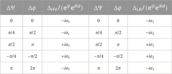
TABLE 3. Summary of the rotated half-wavelength phase-shifter. ΔΨ and Δϕ correspond to rotations in real space and on the Poincaré sphere, respectively. The operators away from the phase factor of ${\mathrm{e}}^{i\beta }{\mathrm{e}}^{i\bar{k}d}$ are listed.

Similarly, the half-wavelength rotator is given by

${\mathcal{D}}_3^{\text{HV}}\left(\mathrm{\Delta }\varphi =\pi \right)=-i{\sigma }_2,(198)$

which is independent on the physical rotation, as we confirmed. These are corresponding to the original Pauli matrices, responsible for these rotations (Table 2).

Another important quantum-mechanical aspect of these rotations are coming from the difference between SU(2) and SO(3) [61,62]. If we consider 2π rotations by successive application of these operators, we confirm the phase change of −1 as

${\mathcal{D}}_1^{\text{HV}}\left({\delta }_{\text{sf}}=\pi \right){\mathcal{D}}_1^{\text{HV}}\left({\delta }_{\text{sf}}=\pi \right)=-{\sigma }_3{\sigma }_3=-\mathbf{1}(199)$

${\mathcal{D}}_2^{\text{HV}}\left({\delta }_{\text{sf}}=\pi \right){\mathcal{D}}_2^{\text{HV}}\left({\delta }_{\text{sf}}=\pi \right)=-{\sigma }_1{\sigma }_1=-\mathbf{1}(200)$

${\mathcal{D}}_3^{\text{HV}}\left({\delta }_{\text{sf}}=\pi \right){\mathcal{D}}_3^{\text{HV}}\left(\mathrm{\Delta }\varphi =\pi \right)=-{\sigma }_2{\sigma }_2=-\mathbf{1}.(201)$

This means that the polarisation control is not classical at all, but fully quantum mechanical. The non-trivial phase change is successfully incorporated in the spin rotation operator of an SU(2) group theory.

We have obtained the same relationship in the LR-basis for the half-wavelength phase-shift, its rotated one, and the half-wavelength rotator, as

${\mathcal{D}}_1^{\text{LR}}\left({\delta }_{\text{sf}}=\pi \right)=-i{\sigma }_1,(202)$

${\mathcal{D}}_2^{\text{LR}}\left({\delta }_{\text{sf}}=\pi \right)=-i{\sigma }_2,(203)$

${\mathcal{D}}_3^{\text{LR}}\left(\mathrm{\Delta }\varphi =\pi \right)=-i{\sigma }_3,(204)$

respectively, which are consistent with Table 2. It is also obvious that the phase change is properly included for 2π rotations, since ${\sigma }_i^2=1$ for ^∀i = 1, 2, 3.

It is also interesting to note that a phase-shifter, which aligns its optical axis (SA or FA) horizontally, is not affected by a flip-flop exchange (Figure 8). This must be true, because the crystal has a mirror symmetry against both SA and FA. Therefore, there is no difference between the front side and the back side with regard to the amount of the polarisation rotation, achieved by the phase-shifter. Nevertheless, the alignment of the SA or FA to the designated direction is important, such that if the phase-shifter is rotated, to align its FA to the diagonal direction, the flip-flop by the mirror symmetric exchange against y-axis will make the FA align to the anti-diagonal direction. This corresponds to rotate in the opposite direction. Still, there is no difference for the half-wavelength phase-shifter, but it does make a difference for a quarter-wavelength phase-shifter.

As an example of the application of the rotated half-wavelength phase-shifter, we consider the input state of |H⟩. In this case, the expectation value of spin by the output state, becomes.

$⟨\mathrm{o}\mathrm{u}\mathrm{t}\mathrm{p}\mathrm{u}\mathrm{t}|\widehat{\mathbf{S}}|\mathrm{o}\mathrm{u}\mathrm{t}\mathrm{p}\mathrm{u}\mathrm{t}⟩=\hslash N\left(\begin{array}{c}\hfill \cos \left(2\mathrm{\Delta }\varphi \right)\hfill \\ \hfill \sin \left(2\mathrm{\Delta }\varphi \right)\hfill \\ \hfill 0\hfill \end{array}\right)$

$=\hslash N\left(\begin{array}{c}\hfill \cos \left(4\mathrm{\Delta }\mathit{\Psi }\right)\hfill \\ \hfill \sin \left(4\mathrm{\Delta }\mathit{\Psi }\right)\hfill \\ \hfill 0\hfill \end{array}\right),(205)$

which means that the average spin vector (Stokes vector) will rotate 4-times on the Poincaré sphere, while rotating the phase-shifter 1-time in real space (ΔΨ changing from 0 to 2π). The trajectory of the Stokes vector is shown in Figure 9. In this case, the Stokes vector is always located in the S₁ − S₂ plane, and the output state will rotate anti-clock-wise, seen from the top of S₃ upon the rotation of the phase-shifter towards the anti-clock-wise, seen from the detector side.

FIGURE 9

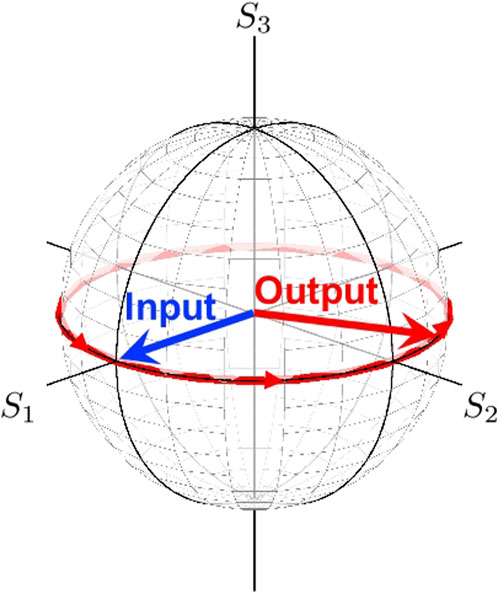
FIGURE 9. The trajectory (red curve along the equator) of the output Stokes vector (red arrow) by the rotated phase-shifter with the input of the horizontally polarised state (blue arrow).

4.4.2 Rotated quarter-wavelength phase-shifters

Another frequently used phase-shifters is a quarter-wavelength phase-shifter at δ_sf = 2π(n_s − n_f)d/λ = π/2, which corresponds to the deference in path lengths of the quarter wavelength between SA and FA. Operators of the quarter-wavelength phase-shifters at major angles are summarised in Table 4.

TABLE 4

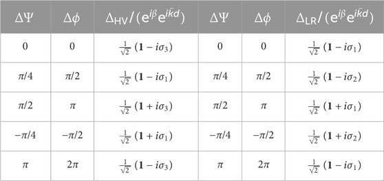
TABLE 4. Summary of the rotated quarter-wavelength phase-shifter. ΔΨ and Δϕ correspond to rotations in real space and on the Poincaré sphere, respectively. The operators away from the phase factor of ${\mathrm{e}}^{i\beta }{\mathrm{e}}^{i\bar{k}d}$ are listed.

An example of the operation using the quarter wavelength phase-shifter is shown in Figure 10. It is crucial to align SA or FA properly for the desired operation, because it determines the direction of rotation whether right (clock-wise) or left (anti-clock-wise) rotations.

FIGURE 10

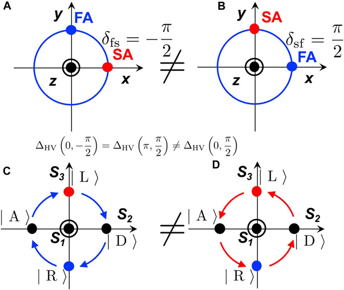
FIGURE 10. The difference of the alignment of the optical axis for the quarter-wavelength phase-shifter. (A) Slow axis (SA) aligned horizontally. (B) Fast axis (FA) aligned horizontally. (C) Rotation of polarisation state (clock-wise rotation, shown by blue curves) on the Poincaré sphere, when SA is aligned horizontally. (D) Rotation of polarisation state (anti-clock-wise rotation, shown by red curves)on the Poincaré sphere, when FA is aligned horizontally.

We can recognise that 2 successive applications of the quarter-wavelength phase-shifters correspond to 1 application of the half-wavelength phase-shifter, except for the global phase.

${\left(\frac{{\mathrm{\Delta }}_{\text{HV}}\left({\delta }_{\text{sf}}=\pi /2\right)}{{\mathrm{e}}^{i\beta }{\mathrm{e}}^{i\bar{k}d}}\right)}^2={\left(\frac{1}{\sqrt{2}}\left(\mathbf{1}-i{\sigma }_3\right)\right)}^2(206)$

$=-i{\sigma }_3(207)$

$=\frac{{\mathrm{\Delta }}_{\text{HV}}\left({\delta }_{\text{sf}}=\pi \right)}{{\mathrm{e}}^{i\beta }{\mathrm{e}}^{i\bar{k}d}},(208)$

because of the additive nature of the rotation, ${\mathcal{D}}_1^{\text{HV}}(\pi /2){\mathcal{D}}_1^{\text{HV}}(\pi /2)={\mathcal{D}}_1^{\text{HV}}(\pi )$, which simply means that 2 quarters-rotations are equivalent to 1 half-rotation. Mathematically, this means that the rotational operations form a group. Consequently, 4 quarters-rotations are equivalent to 1-whole-rotation on the Poincaré sphere, which yields ${\left({\mathcal{D}}_1^{\text{HV}}(\pi /2)\right)}^4=-1$.

In Figure 11, we show the trajectories of the output polarisation state, $⟨\mathrm{o}\mathrm{u}\mathrm{t}\mathrm{p}\mathrm{u}\mathrm{t}|\widehat{\mathbf{S}}|\mathrm{o}\mathrm{u}\mathrm{t}\mathrm{p}\mathrm{u}\mathrm{t}⟩$, when the linearly polarised input states are rotated by the rotated quarter-wavelength phase-shifters. Upon physically-rotating the phase-shifter, the linearly polarised state changes its ellipticity, arriving to the poles, which correspond to left- and right-circularly polarised states, and coming back to the original state. For example, if the input is the horizontally polarised state, the output spin becomes

$⟨\mathrm{o}\mathrm{u}\mathrm{t}\mathrm{p}\mathrm{u}\mathrm{t}|\widehat{\mathbf{S}}|\mathrm{o}\mathrm{u}\mathrm{t}\mathrm{p}\mathrm{u}\mathrm{t}⟩=\hslash N\left(\begin{array}{c}\hfill {\cos }^2\left(\mathrm{\Delta }\varphi \right)\hfill \\ \hfill \sin \left(\mathrm{\Delta }\varphi \right)\cos \left(\mathrm{\Delta }\varphi \right)\hfill \\ \hfill -\sin \left(\mathrm{\Delta }\varphi \right)\hfill \end{array}\right).(209)$

FIGURE 11

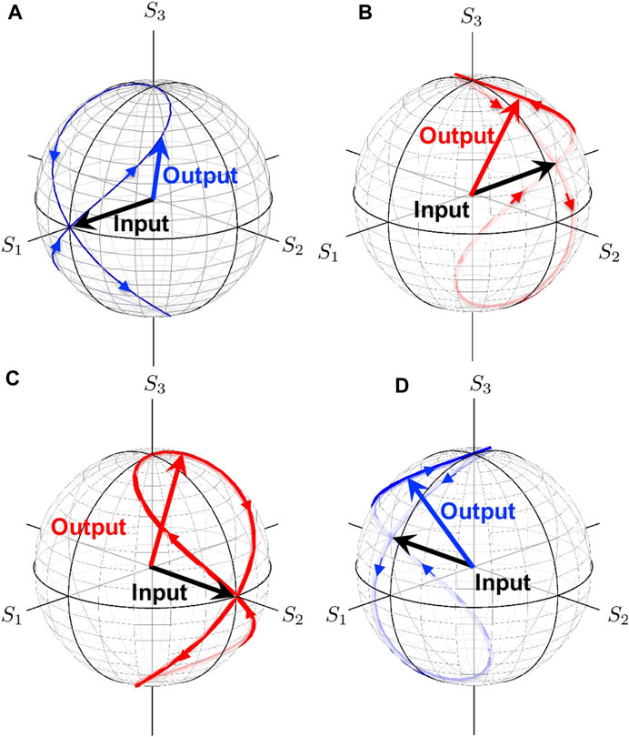
FIGURE 11. Trajectories of output polarisation states by the rotated quarter-wavelength phase-shifters. The input is linearly polarised state. (A) The input is a horizontally polarised state, |H⟩. The trajectory is shown by the blue curve. (B) The input is a vertically polarised state, |V⟩. The trajectory is shown by the red curve. (C) The input is a diagonally polarised state, |D⟩. The trajectory is shown by the red curve. (D) The input is an anti-diagonally polarised state, |A⟩. The trajectory is shown by the blue curve.

while physically-rotating the quarter-wavelength phase-shifter 1-time in real space, the Stokes vector will rotate 2-times, because Δϕ = 2ΔΨ. The horizontally polarised state can never arrive to be the vertically polarised state by the quarter-wavelength phase-shifter, because the horizontally polarised state does not contain any contribution of the orthogonal vertically polarised state and the π/4 change of the phase-shift is not large enough.

4.5 Polariser

So far, we have discussed phase-shifters and rotators, which are described energy-conserving unitary operators. The advantages of Jones vector treatments are the capabilities to extend the operator analysis to the situations with energy-dissipations. One of the most important polarisation optical components in that aspect is a polariser [5,21,22,28]. Polarisers are made, for example, by patterning thin metallic layer into arrays of metallic wires with sub-wavelength widths [74]. This allows to reflect and absorb the most of the polarisation component along the direction of the long axis of the wires, while the polarisation component perpendicular to the wires can transmit the polariser. There are many other types of polarisers by using polymers with polarisation-dependent absorption coefficients or reflectors using birefringent prisms or reflections at Brewster’s angle.

4.5.1 Polariser in the HV-basis

It is straightforward to consider a polariser operator in the HV-basis,

${\widehat{\mathcal{P}}}_x^{\text{HV}}={\mathrm{e}}^{i{k}_0{n}_{x}d-{\alpha }_{x}d}\frac{{\mathrm{e}}^{i\beta }}{\sqrt{N}}{\widehat{a}}_{\text{H}}\widehat{\mathbf{x}}+{\mathrm{e}}^{i{k}_0{n}_{y}d-{\alpha }_{y}d}\frac{{\mathrm{e}}^{i\beta }}{\sqrt{N}}{\widehat{a}}_{\text{V}}\widehat{\mathbf{y}},(210)$

where n_x and n_y are refractive indices, and α_x and α_y are absorption coefficients per unit propagation length for polarisation components along x and y, respectively, and d is the thickness of the polariser. For the ideal horizontal polariser, we take the limits of α_xd → 1 and α_yd → ∞, and we obtain

${\widehat{\mathcal{P}}}_x^{\text{HV}}={\mathrm{e}}^{i\bar{k}d}\frac{{\mathrm{e}}^{i\beta }}{\sqrt{N}}{\widehat{a}}_{\text{H}}\widehat{\mathbf{x}},(211)$

where $\bar{k}=k_0{n}_x$. By considering the spinor representation of the output state, we obtain

$|\mathrm{o}\mathrm{u}\mathrm{t}\mathrm{p}\mathrm{u}\mathrm{t}\rangle ={\widehat{\mathcal{P}}}_x^{\text{HV}}|{\alpha }_{\text{H}},{\alpha }_{\text{V}}\rangle$

$={\mathrm{e}}^{i\beta }{\mathrm{e}}^{i\bar{k}d}\left(\begin{array}{cc}\hfill 1\hfill & \hfill 0\hfill \\ \hfill 0\hfill & \hfill 0\hfill \end{array}\right)\left(\begin{array}{c}\hfill {\mathrm{e}}^{-i\frac{\delta }{2}}\cos \alpha \hfill \\ \hfill {\mathrm{e}}^{+i\frac{\delta }{2}}\sin \alpha \hfill \end{array}\right)|\mathrm{i}\mathrm{n}\mathrm{p}\mathrm{u}\mathrm{t}\rangle .(212)$

Therefore, we obtain

$\begin{array}{ccc}\hfill & \hfill & \langle {\alpha }_{\text{H}},{\alpha }_{\text{V}}|{\widehat{\mathcal{P}}}_x^{\text{HV}}|{\alpha }_{\text{H}},{\alpha }_{\text{V}}\rangle \hfill \\ \hfill & \hfill & ={\mathrm{e}}^{i\beta }{\mathrm{e}}^{i\bar{k}d}\left(\begin{array}{cc}\hfill 1\hfill & \hfill 0\hfill \\ \hfill 0\hfill & \hfill 0\hfill \end{array}\right)\left(\begin{array}{c}\hfill {\mathrm{e}}^{-i\frac{\delta }{2}}\cos \alpha \hfill \\ \hfill {\mathrm{e}}^{+i\frac{\delta }{2}}\sin \alpha \hfill \end{array}\right)\hfill \end{array}(213)$

$={\mathcal{P}}_x^{\text{HV}}|\mathrm{J}\mathrm{o}\mathrm{n}\mathrm{e}\mathrm{s}\rangle ,(214)$

where we have defined the Jones matrix for the horizontal polariser as

${\mathcal{P}}_x^{\text{HV}}={\mathrm{e}}^{i\beta }{\mathrm{e}}^{i\bar{k}d}\left(\begin{array}{cc}\hfill 1\hfill & \hfill 0\hfill \\ \hfill 0\hfill & \hfill 0\hfill \end{array}\right)(215)$

$=\frac{{\mathrm{e}}^{i\beta }{\mathrm{e}}^{i\bar{k}d}}{2}\left(\mathbf{1}+{\sigma }_z\right).(216)$

Similarly, we obtain the Jones matrix for vertical polariser as.

${\mathcal{P}}_y^{\text{HV}}={\mathrm{e}}^{i\beta }{\mathrm{e}}^{i\bar{k}d}\left(\begin{array}{cc}\hfill 0\hfill & \hfill 0\hfill \\ \hfill 0\hfill & \hfill 1\hfill \end{array}\right)(217)$

$=\frac{{\mathrm{e}}^{i\beta }{\mathrm{e}}^{i\bar{k}d}}{2}\left(\mathbf{1}-{\sigma }_z\right).(218)$

It is important to recognise that polarisers are projectors to remove one of the orthogonal components, and the intensity of the ray will be reduced, accordingly. Consequently, it is dissipative irreversible operation, and thus the inverse of the polariser matrix does not exist. It is also interesting to note that the transmitted output state is not altered except for the global phase of ${\mathrm{e}}^{i\beta }{\mathrm{e}}^{i\bar{k}d}$.

4.5.2 Polariser in the LR-basis

After obtaining the polariser operators in the HV-basis, it is straightforward to obtain the corresponding operators in the LR-basis simply by unitary transformations. We obtain

${\mathcal{P}}_x^{\text{LR}}=U_{\text{HV}}^{-1}{\mathcal{P}}_x^{\text{HV}}{U}_{\text{HV}}(219)$

$=\frac{{\mathrm{e}}^{i\bar{k}d}}{2}\left(\begin{array}{cc}\hfill 1\hfill & \hfill -i\hfill \\ \hfill 1\hfill & \hfill i\hfill \end{array}\right)\left(\begin{array}{cc}\hfill 1\hfill & \hfill 0\hfill \\ \hfill 0\hfill & \hfill 0\hfill \end{array}\right)\left(\begin{array}{cc}\hfill 1\hfill & \hfill 1\hfill \\ \hfill i\hfill & \hfill -i\hfill \end{array}\right)(220)$

$=\frac{{\mathrm{e}}^{i\bar{k}d}}{2}\left(\begin{array}{cc}\hfill 1\hfill & \hfill 1\hfill \\ \hfill 1\hfill & \hfill 1\hfill \end{array}\right)(221)$

$=\frac{{\mathrm{e}}^{i\bar{k}d}}{2}\left(\mathbf{1}+{\sigma }_x\right),(222)$

and

${\mathcal{P}}_y^{\text{LR}}=U_{\text{HV}}^{-1}{\mathcal{P}}_y^{\text{HV}}{U}_{\text{HV}}(223)$

$=\frac{{\mathrm{e}}^{i\bar{k}d}}{2}\left(\begin{array}{cc}\hfill 1\hfill & \hfill -i\hfill \\ \hfill 1\hfill & \hfill i\hfill \end{array}\right)\left(\begin{array}{cc}\hfill 0\hfill & \hfill 0\hfill \\ \hfill 0\hfill & \hfill 1\hfill \end{array}\right)\left(\begin{array}{cc}\hfill 1\hfill & \hfill 1\hfill \\ \hfill i\hfill & \hfill -i\hfill \end{array}\right)(224)$

$={\mathrm{e}}^{i\bar{k}d}\left(\begin{array}{cc}\hfill 1\hfill & \hfill -1\hfill \\ \hfill -1\hfill & \hfill 1\hfill \end{array}\right)(225)$

$=\frac{{\mathrm{e}}^{i\bar{k}d}}{2}\left(\mathbf{1}-{\sigma }_x\right).(226)$

4.5.3 Rotated polarisers

It is also straightforward to obtain the rotated polarisers with the angle of ΔΨ = Δϕ/2. In the HV-basis, it becomes

${\mathcal{P}}_x^{\text{HV}}\left(\mathrm{\Delta }\varphi \right)=R_{\text{HV}}\left(\mathrm{\Delta }\mathit{\Psi }\right){\mathcal{P}}_x^{\text{HV}}{R}_{\text{HV}}\left(-\mathrm{\Delta }\mathit{\Psi }\right)(227)$

$=\frac{{\mathrm{e}}^{i\bar{k}d}}{2}\left(\begin{array}{cc}\hfill 1+\cos \left(\mathrm{\Delta }\varphi \right)\hfill & \hfill \sin \left(\mathrm{\Delta }\varphi \right)\hfill \\ \hfill \sin \left(\mathrm{\Delta }\varphi \right)\hfill & \hfill 1-\cos \left(\mathrm{\Delta }\varphi \right)\hfill \end{array}\right).(228)$

In the LR-basis, it becomes

${\mathcal{P}}_x^{\text{LR}}\left(\mathrm{\Delta }\varphi \right)=R_{\text{LR}}\left(\mathrm{\Delta }\mathit{\Psi }\right){\mathcal{P}}_x^{\text{LR}}{R}_{\text{LR}}\left(-\mathrm{\Delta }\mathit{\Psi }\right)(229)$

$=\frac{{\mathrm{e}}^{i\bar{k}d}}{2}\left(\begin{array}{cc}\hfill 1\hfill & \hfill {\mathrm{e}}^{-i\Delta \varphi }\hfill \\ \hfill {\mathrm{e}}^{i\Delta \varphi }\hfill & \hfill 1\hfill \end{array}\right).(230)$

The rotated polarisers at typical angles are summarised in Table 5.

TABLE 5

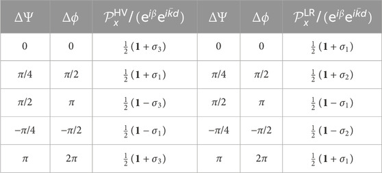
TABLE 5. Summary of the rotated polarisers. ΔΨ and Δϕ correspond to rotations in real space and on the Poincaré sphere, respectively. The operators away from the phase factor of ${\mathrm{e}}^{i\beta }{\mathrm{e}}^{i\bar{k}d}$ are listed.

4.6 Difference between SU(2) and SO(3)

We think it is worth for summarising our simple picture on the difference between SU(2) and SO(3) [61,62] for polarisation states [60]. We consider a situation, where the Stokes vector rotate 1-time on the Poincaré sphere (Figure 12). Suppose this could be achieved by phase-shifters, e.g., by 2 successive operations of the half-wavelength phase-shifters. The spin expectation value, $⟨\mathrm{o}\mathrm{u}\mathrm{t}\mathrm{p}\mathrm{u}\mathrm{t}|\widehat{\mathbf{S}}|\mathrm{o}\mathrm{u}\mathrm{t}\mathrm{p}\mathrm{u}\mathrm{t}⟩$, would not be changed upon this rotation, such that the polarisation state is equivalent in terms of the expectation value. However, the electric field has changed its sign, such that the destructive interference can be observable upon the coupling to the original wave before the rotation. We could successfully include this phase change in our SU(2) description of the spin state of photons, because ${\mathcal{D}}_1^{\text{HV}}({\delta }_{\text{sf}}=2\pi )=-1$.

FIGURE 12

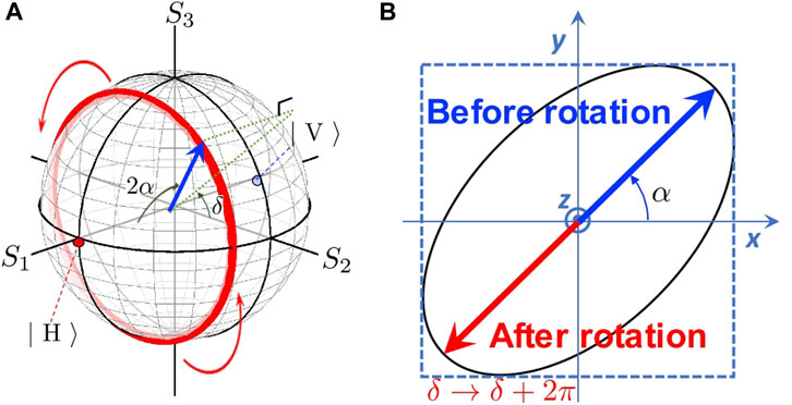
FIGURE 12. The impact of phase change upon the rotation. (A) 1-time rotation of the Stokes vector in Poincareé sphere. The polarisation state, seen from the average of the expectation value, is not changed at all upon the rotation (red curve). (B) The corresponding polarisation ellipse, in the real space. The electric field before rotation (blue arrow) is pointing to the opposite direction after rotation (red curve). The sign of the electric field changes both for x and y directions. This change of the phase is different from the global phase coming from the orbital, and thus, the phase change can be observed by the interference with the original wave before the rotation.

The acquisition of this phase upon the 1-time rotation does not depend on how we rotate the polarisation state nor the bases which we are going to use. Let us consider to use the chiral LR-basis and rotate the polarisation state (θ, ϕ) 1-time upon rotating θ to θ − 2π (Figure 13A). This corresponds to use the rotation axis, which is rotated to the clock-wise with the amount of Δϕ′ = π/2 − ϕ from S₁. Therefore, the rotation axis is pointing to n = (cos (−Δϕ′), sin (−Δϕ′), 0), which corresponds to rotate the phase-shifter with the amount of ΔΨ′ = π/4 − ϕ/2 in the clock-wise direction (Figure 13B). Upon this 2π rotation on the Poincaré sphere, the spin expectation value will not be changed, since the spin is coming back to point to the original direction. However, the electric field in the polarisation ellipse changes its sign in the polarisation ellipse (Figure 13D), because the rotation corresponds to rotate χ with the amount of π. This difference of the factor of 2 among θ in the Poincaré sphere and χ in the polarisation ellipse is responsible for the emergence of the geometrical phase. In an SU(2) theory, this simply corresponds to ${\mathcal{D}}^{\text{LR}}(\mathbf{n},{\delta }_{\text{sf}}=2\pi )=-1$.

FIGURE 13

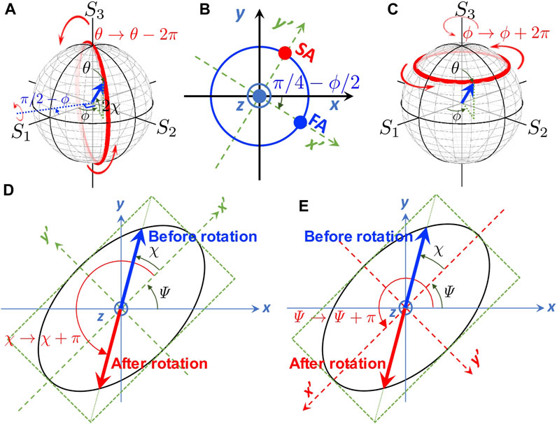
FIGURE 13. The phase change, seen from the chiral bases. (A) 1-time rotation of the Stokes vector by the phase-shifter in Poincareé sphere (red curve). The polarisation state is not changed upon the rotation. (B) Corresponding phase-shifter arrangement, showing the x′-y′ axes are rotated (dotted green). (C) 1-time rotation of the Stokes vector by a rotator in Poincareé sphere (red curve). (D) Corresponding polarisation ellipse after the rotation by the phase-shifter of (A) and (B). (E) Corresponding polarisation ellipse after the rotation by the rotator of (C). In all cases, 1-time rotation will induce the sign change for the complex electric fields, which is proportional to the SU(2) wavefunction.

We can also confirm the impact of the polarisation rotation by a rotator, which is equivalent to the adiabatic change of the coordinate (Figure 13C). The rotation corresponds to change ϕ to be ϕ + 2π around S₃. This corresponds to rotate the inclination angle Ψ with the amount of π, because ϕ = 2Ψ (Figure 13E). In an SU(2) theory, it is guaranteed by ${\mathcal{D}}_3^{\text{LR}}({\delta }_{\text{sf}}=2\pi )=-1$.

Away from the global U (1) phase factor of ${\mathrm{e}}^{i\beta }{\mathrm{e}}^{i\bar{k}d}$, the sign of the rotator operation depends on the direction of rotation, because ${\mathcal{D}}_3^{\text{LR}}(\pi )=-i{\sigma }_3$ and ${\mathcal{D}}_3^{\text{LR}}(-\pi )=+i{\sigma }_3$. This is equivalent to the difference of the 2π for the rotation. The difference of the sign of the operators are indispensable to guarantee the identity, ${\mathcal{D}}_3^{\text{LR}}(\pi ){\mathcal{D}}_3^{\text{LR}}(-\pi )={\mathcal{D}}_3^{\text{LR}}(0)={\sigma }_3^2=\mathbf{1}$. We can also confirm this in HR-basis as ${\mathcal{D}}_3^{\text{HR}}(\pi )=-i{\sigma }_2$ and ${\mathcal{D}}_3^{\text{HR}}(-\pi )=+i{\sigma }_2$, and consequently ${\mathcal{D}}_3^{\text{HR}}(\pi ){\mathcal{D}}_3^{\text{HR}}(-\pi )={\mathcal{D}}_3^{\text{HR}}(0)={\sigma }_2^2=\mathbf{1}$.

Another quantum-mechanical aspect of the spin of photons is found by successive application of rotation operations on the Poincaré sphere (Figure 14). We have confirmed that the half-wavelength phase-shifters and the rotator are equivalent to Pauli matrices,

$i{\mathcal{D}}_i^{\text{LR}}\left(\pi \right)={\sigma }_i,(231)$

where i = 1, 2, 3, which obey commutation and anti-commutation relationships. The commutation relationship is a fundamental basis of quantum-mechanics and thus it is also essential for spin of photons. For polarisation, we can easily manipulate spin of photons by phase-shifter and rotators, but it is important to aware the order is important, because the sign can be changed as

FIGURE 14

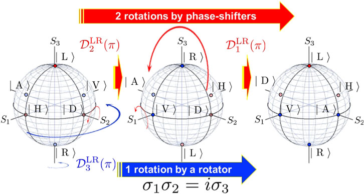
FIGURE 14. Equivalence of 2 half-wavelength phase-shifter operators (red arrows) and 1 half-wavelength rotator operation (blue arrow). We considered the phase-shifter rotation along S₂ and the successive rotation along S₁ in chiral LR-basis (red arrows). This is equivalent to the 1-rotation along S₃ by a rotator (blue arrow). It is important to consider the overall phase by this operation, since this corresponds to σ₁σ₂ = −σ₂σ₁ = iσ₃, which depends on the order of operations. In HR-basis, this corresponds to σ₃σ₁ = −σ₁σ₃ = iσ₂.

This shows that 2 successive rotations by phase-shifters, one aligned its FA to the diagonal direction and the other aligned its FA to the horizontal direction, are equivalent to 1 rotation by a rotator. We can change the order of operations, without changing the final polarisation state as an expectation value of the spin operators. However, the phase is different depending on the order of applications of the phase-shifters. This difference of the sign should also be observable in the interference experiments. Essentially, this is equivalent to the difference of 1-time rotation by a rotator, because iσ₃ and −iσ₃ correspond to the rotation of π and −π, respectively, such that the difference is 2π-rotation, as we have explained above.

4.7 Jones vector and bloch vector in SU(2) hilbert space

As we have seen above, an SU(2) group theory is a powerful tool to understand various rotations of $⟨\widehat{\mathbf{S}}⟩$ on the Poincaré sphere. Here, we apply an SU(2) group theory to confirm some of concepts for polarisation states.

First, we obtain the unitary transformation from the HV-basis to the LR-basis by rotators in the SU(2) Hilbert space. The choice of the bases is based on our preference of the quantisation axis. The HV-basis is based on the alignment of the quantisation axis σ₃ to the S₁ axis (Table 2), while the LR-basis is based on the alignment of σ₃ to the S₃ axis (Figures 15A, B). The expectation values should not depend on the choice of the basis, such that we should be able to transfer from the HV-basis to the LR-basis by a unitary transformation, which is described by the following 2 steps of rotations. First, we start from the HV-basis and apply the rotation along S₂ for the amount of −π/2 as

${\mathcal{D}}_2^{\text{HV}}\left(-\frac{\pi }{2}\right)=\frac{1}{\sqrt{2}}\left(\mathbf{1}+i{\sigma }_x\right)=\frac{1}{\sqrt{2}}\left(\begin{array}{cc}\hfill 1\hfill & \hfill i\hfill \\ \hfill i\hfill & \hfill 1\hfill \end{array}\right).(232)$

FIGURE 15

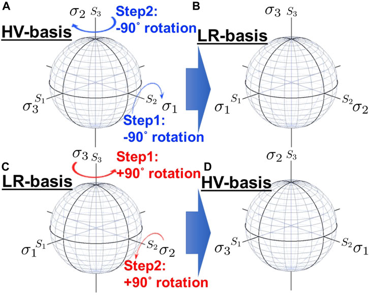
FIGURE 15. Unitary transformation between linear horizontal/vertical (HV)-basis and chiral left/right (LR)-basis. (A) Original HV-basis. In order to convert HV-basis to LR-basis, we consider 2 operations: the first step is to rotate −90° along the S₂ axis and the second step is to rotate −90° along the S₃. (B) Rotated LR-basis. (C) Original LR-basis. In order to bring LR-basis back to HV-basis, we consider 2 operations: the first step is to rotate +90° along the S₃ axis and the second step is to rotate 90° along the S₂. (D) Rotated HV-basis.

Next, we rotate along the S₃ for the amount of −π/2 as

${\mathcal{D}}_3^{\text{HV}}\left(-\frac{\pi }{2}\right)=\frac{1}{\sqrt{2}}\left(\mathbf{1}+i{\sigma }_y\right)=\frac{1}{\sqrt{2}}\left(\begin{array}{cc}\hfill 1\hfill & \hfill 1\hfill \\ \hfill -1\hfill & \hfill 1\hfill \end{array}\right).(233)$

These 2 successive rotations in SU(2) space give the unitary

$U_{\text{HV}}={\mathcal{D}}_3^{\text{HV}}\left(-\frac{\pi }{2}\right){\mathcal{D}}_2^{\text{HV}}\left(-\frac{\pi }{2}\right)(234)$

$=\frac{1}{2}\left(\begin{array}{cc}\hfill 1\hfill & \hfill 1\hfill \\ \hfill -1\hfill & \hfill 1\hfill \end{array}\right)\left(\begin{array}{cc}\hfill 1\hfill & \hfill i\hfill \\ \hfill i\hfill & \hfill 1\hfill \end{array}\right)(235)$

$=\frac{{\mathrm{e}}^{i\pi /4}}{\sqrt{2}}\left(\begin{array}{cc}\hfill 1\hfill & \hfill 1\hfill \\ \hfill i\hfill & \hfill -i\hfill \end{array}\right),(236)$

which is in agreement with the previous result away from the irrelevant overall U (1) phase factor of e^iπ/4.

Similarly, we also confirmed the inverse transformation (Figures 15C, D) as

$U_{\text{LR}}={\mathcal{D}}_2^{\text{LR}}\left(\frac{\pi }{2}\right){\mathcal{D}}_3^{\text{LR}}\left(\frac{\pi }{2}\right)(237)$

$=\frac{1}{2}\left(\begin{array}{cc}\hfill 1\hfill & \hfill -1\hfill \\ \hfill 1\hfill & \hfill 1\hfill \end{array}\right)\left(\begin{array}{cc}\hfill {\mathrm{e}}^{-i\pi /4}\hfill & \hfill 0\hfill \\ \hfill 0\hfill & \hfill {\mathrm{e}}^{i\pi /4}\hfill \end{array}\right)(238)$

$=\frac{{\mathrm{e}}^{-i\pi /4}}{\sqrt{2}}\left(\begin{array}{cc}\hfill 1\hfill & \hfill -i\hfill \\ \hfill 1\hfill & \hfill i\hfill \end{array}\right).(239)$

Finally, we obtain the Jones vector and the Bloch vector by the rotations in an SU(2) Hilbert space. For Jones vector, we use the linear HV-basis, and start from |H⟩. Then, we will rotate along S₃ with the amount of γ, and then subsequently rotate along S₁ with the amount of δ. Consequently, we obtain

$|\gamma ,\delta \rangle ={\mathcal{D}}_1^{\text{HV}}\left(\delta \right){\mathcal{D}}_3^{\text{HV}}\left(\gamma \right)|\mathrm{H}\rangle (240)$

$=\left(\begin{array}{cc}\hfill {\mathrm{e}}^{-i\frac{\delta }{2}}\hfill & \hfill 0\hfill \\ \hfill 0\hfill & \hfill {\mathrm{e}}^{+i\frac{\delta }{2}}\hfill \end{array}\right)\left(\begin{array}{cc}\hfill \cos \left(\frac{\gamma }{2}\right)\hfill & \hfill -\sin \left(\frac{\gamma }{2}\right)\hfill \\ \hfill \sin \left(\frac{\gamma }{2}\right)\hfill & \hfill \cos \left(\frac{\gamma }{2}\right)\hfill \end{array}\right)\left(\begin{array}{c}\hfill 1\hfill \\ \hfill 0\hfill \end{array}\right)$

$=\left(\begin{array}{c}\hfill {\mathrm{e}}^{-i\frac{\delta }{2}}\cos \left(\frac{\gamma }{2}\right)\hfill \\ \hfill {\mathrm{e}}^{+i\frac{\delta }{2}}\sin \left(\frac{\gamma }{2}\right)\hfill \end{array}\right)(241)$

$=|\mathrm{J}\mathrm{o}\mathrm{n}\mathrm{e}\mathrm{s}\rangle ,(242)$

Which is indeed the Jones vector.

For Bloch state, we start from the chiral LR-basis, and start from |L⟩. Then, we rotate the state along S₂ with the amount of θ and rotate it along S₃ with the amount of ϕ. Thus, we obtain

$|\theta ,\varphi \rangle ={\mathcal{D}}_3^{\text{LR}}\left(\varphi \right){\mathcal{D}}_2^{\text{LR}}\left(\theta \right)|\mathrm{L}\rangle (243)$

$=\left(\begin{array}{cc}\hfill {\mathrm{e}}^{-i\frac{\varphi }{2}}\hfill & \hfill 0\hfill \\ \hfill 0\hfill & \hfill {\mathrm{e}}^{+i\frac{\varphi }{2}}\hfill \end{array}\right)\left(\begin{array}{cc}\hfill \cos \left(\frac{\theta }{2}\right)\hfill & \hfill -\sin \left(\frac{\theta }{2}\right)\hfill \\ \hfill \sin \left(\frac{\theta }{2}\right)\hfill & \hfill \cos \left(\frac{\theta }{2}\right)\hfill \end{array}\right)\left(\begin{array}{c}\hfill 1\hfill \\ \hfill 0\hfill \end{array}\right)$

$=\left(\begin{array}{c}\hfill {\mathrm{e}}^{-i\frac{\varphi }{2}}\cos \left(\frac{\theta }{2}\right)\hfill \\ \hfill {\mathrm{e}}^{+i\frac{\varphi }{2}}\sin \left(\frac{\theta }{2}\right)\hfill \end{array}\right)(244)$

$=|\mathrm{B}\mathrm{l}\mathrm{o}\mathrm{c}\mathrm{h}\rangle ,(245)$

which is the Bloch state. Therefore, polarisation states are described by spin states and operators based on an SU(2) group theory.

4.8 Spin textures and classical entanglement

So far we have discussed coherent photons of a single mode to discuss about the origin of polarisation in a frame work of a quantum field theory with an SU(2) symmetry [1–9,20–24,45–47,64–72]. It is beyond the scope of this work to include multiple modes with orbital angular momentum for discussing about the higher-order Poincaré sphere [12,75–85]. However, many important progresses are being made in the area of spin textures [86–90] and classical entanglement [39,91–97], such that we would like to outline how our theory will be extended to discuss these effects for the future [71,98,99].

In order to allow the higher order modes in addition to the lowest order Gaussian mode [5,21–24], we must realise these modes are orthogonal to each other. One might think this is trivial requirement for quantum mechanics [7–9] or multi-mode analyses [5,21–24], however, it is less trivial for orbital angular momentum of photons [11,13–15,18–20], since a lot of researchers are thinking that the splitting is impossible. In order to identify the condition for allowing the splitting, we have considered propagation in a graded-index fibre, where exact solutions are available [20]. Then, we found that the splitting of spin and orbital angular momentum is possible in the waveguide, and the splitting is justified as far as the ray is sufficiently collimated to justify the finite mode profile, which induces a small longitudinal component to allow the splitting [20]. If the condition is satisfied, we can treat orbital angular momentum as an independent degree of freedom from spin to form structured lights [12,40,46,47,75–85,94,95,100,101].

In order to discuss structured lights in our theoretical framework of a quantum field theory, we need to extend the SU(2) symmetry to have the SU$(\mathcal{N})$ symmetry with degree $\mathcal{N}>2$ [6,9,69,71,72,98,99,102–110]. We are developing both theoretical [71] and experimental [72,98,99] platforms to discuss coherent photons with the higher order SU$(\mathcal{N})$ symmetry.

5 Conclusion

We have discussed what is spin of a photon? Our hypothesis is that spin of a photon is an intrinsic quantum-mechanical degree of freedom inherent to a photon, which was suggested by the classical description of the angular momentum expression together with the Poynting vector. We obtained the chiral spin component by this analogy. We have accepted as a principle, that the chiral spin operator of a photon is aligned to the direction of propagation, and applied a standard quantum-mechanical prescription and an SU(2) group theory, assuming the spin state of a photon is described by a two-level quantum-mechanical system. Then, by a rotation in the SU(2) Hilbert space, we obtained all three spatial components of the spin operator, and established that the quantum-mechanical expectation values of the spin of photons are Stokes parameters on the Poincaré sphere. Based on this analogy and the comparison with coherent state of a monochromatic ray of photons from a laser, we identified that the zero-th component of Stokes parameter, S₀, is the order parameter of the coherent ray, which becomes zero after the time average below the lasing threshold, while it becomes finite after the on-set of lasing. The reason why the laser beam is described by a single mode is deeply rooted to the Bose-Einstein condensation nature of photons, which allow macroscopic number of photons occupy the same level with the phase coherence including polarisation states. Based on this identification, the description of Stokes parameters in Poincaré shpere corresponds to the visualisation of the spin expectation values for three spatial components of the vectorial order parameters. There is no obvious contradiction or a difficulty, as far as we accept the spin operators of photons exist as quantum-mechanical many-body operators, and evaluate their expectation values by a coherent state. This does not necessarily mean that the principle to define the spin operators is true, however, with the definition of the spin operators and a standard quantum many-body theory, we can practically deal and understand polarisation states as standard quantum-mechanical states in a two-level system.

We admit that the most of our equations presented in this paper were already appeared in research papers and textbooks on photonics. Nevertheless, it was not completely clear for us to explain the nature of spin of a photon. The situation might have some similarity with the development of the special theory of relativity by Einstein [111], for which the Lorentz transformation [112] was known at that time, while its actual implication on the principle of relativity was not established, yet. Therefore, the equations were not enough to understand the principle behind them. The theory of relativity established the principle that the speed of light, thus, the momentum of a photon in a vacuum is invariant under the Lorentz transformation. The principle behind our SU(2) theory of a photon is the rotational symmetry of the angular momentum of a photon in a vacuum. In other words, there is no particular preferential polarisation state for a photon to be realised in a vacuum, no matter which direction the photon is propagating along with. The rotational symmetry is broken for the coherent light from a laser source, considered in this paper, in the sense that some fixed polarisation state is chosen when the Bose-Einstein condensation of photons occurred upon exceeding the threshold of pumping for lasing. In a material with a broken directional symmetry (phase-shifter) or a broken rotational symmetry (rotator), the polarisation state can be rotated, because of the difference of the phases acquired during the transmission of the material between the orthogonal components of the polarisation state. A remarkable difference from the time of Einstein was that we have almost everything we need to consider the spin of a photon, such as quantum many-body theories, coherent state descriptions, spinor representation, Jones vectors, and so on. We have just applied the existing framework of the quantum field theory to a coherent state of photons to understand the spin state of the photons in a straightforward way.

Now, we have a clear view in confidence that the spin of a photon is well-defined quantum-mechanical observable and the Jones vector is equivalent to the Bloch vector to describe the quantum-mechanical state of polarisation. Thus, the Poincaré sphere is essentially equivalent to the Bloch sphere. The only possible difference between the Poincaré sphere and the Bloch sphere is the statistics of the particles, which we are dealing with; Stokes parameters are used for photons, which are Bose particles, while the Bloch sphere is usually used for the spin state of an electron, which is a Fermi particle. Because of the Bose-Einstein nature of a coherent ray of photons, we obtained the magnitude of the order parameter as S₀ = ℏN, which is macroscopically large compared with ℏ/2 for an electron. What is intriguing is that the quantum-mechanical feature of a spin state of photons is controllable by conventional optical components such as phase-shifters and rotators. It is surprising that the macroscopic coherent state of a laser beam is so easily controlled, and the standard quantum-mechanical operations for a two-level system work successfully for the ray. We hope that we have justified the treatment of Stokes parameters, based on a standard many-body quantum theory and an SU(2) group theory. The commutation relationship of these spin operators are obtained, with the additional factor of two due to the peculiar situation, that a photon has the spin of 1 but only two orthogonal states are allowed due to the transverse condition of the ray. Linear and chiral bases are mutually transferred by unitary transformations, and Jones vector is obtained by the rotation of states in SU(2) Hilbert space.

We have also found that the phase change upon the rotation is essential to consider the commutation relationship of spin state of a photon beyond the expectation value. The 2π rotation in the Poincaré sphere resulted in the π rotation of the electric field in the real space, such that the phase can destructively interfere with the original wave before the rotation, regardless of the same expectation values of the spin. It is required to rotate 4π in the Poincaré sphere to come back to the original polarisation state with the same phase, which is indeed coming from the quantum-mechanical character governed by the commutation relationship. We can also regard that the phase change upon the rotation guarantees non-Abelian relationship of the spin operators for photons.

It is remarkable that Stokes and Poincaré could arrive to the correct formulas, before the establishments of quantum-mechanics, a quantum many-body theory, Maxwell equations, a Ginzburg–Landau theory, Jones vector calculus, and so on. They have captured all important aspects of polarisation states, and certainly, acquired quantum-mechanical nature of polarisation states. In the modern perspective, the remaining challenge for us is to justify the splitting of spin and orbital angular momentum [11,13–15,18,19] at least for photons in a coherent monochromatic state from a laser source. This is not a trivial task at all, and we will revisit this issue, separately.

In conclusion, we believe that spin of a photon is an intrinsic quantum mechanical degree of freedom for polarisation. We accepted the principle that the chiral spin state of a photon is aligned to the direction of the propagation, and applied a many-body quantum field theory to obtain the other spin operators. We cannot derive the spin commutation relationship from a correspondence from classical mechanics. Instead, we accepted the validity of the quantum commutation relationship as a principle for a polarisation state of a photon. It is important to recognise that photons can take any polarisation state, described by a superposition state of the arbitrary chosen two orthogonal polarisation states (e.g., left/right circularly polarised states or horizontal/vertical linearly polarised states), depending on how the coherent ray of photons from a laser source is prepared. We confirmed that the expectation values of the spin components are equivalent to the Stokes parameters, $⟨\widehat{\mathbf{S}}⟩=\mathbf{S}$. Therefore, the Stokes parameters are vectorial order parameters on the Poincaré sphere to describe the coherent nature of photons. It is also important to recognise that we obtained the proportionality constant of the Stokes parameter as ℏN for the spin expectation value. This means that ℏ becomes effectively macroscopic to ℏN for coherent monochromatic photons from a laser source due to the Bose-Einstein condensation. Therefore, we conclude that the polarisation is a macroscopic manifestation of a quantum-mechanical feature of photons.

Data availability statement

The raw data supporting the conclusion of this article will be made available by the authors, without undue reservation.

Author contributions

The author confirms being the sole contributor of this work and has approved it for publication.

Funding

This work is supported by JSPS KAKENHI Grant Number JP 18K19958.

Acknowledgments

The author would like to express sincere thanks to Prof I. Tomita for continuous discussions and encouragements.

Conflict of interest

Author SS was employed by Hitachi Ltd.

Publisher’s note

All claims expressed in this article are solely those of the authors and do not necessarily represent those of their affiliated organizations, or those of the publisher, the editors and the reviewers. Any product that may be evaluated in this article, or claim that may be made by its manufacturer, is not guaranteed or endorsed by the publisher.

Supplementary material

The Supplementary Material for this article can be found online at: https://www.frontiersin.org/articles/10.3389/fphy.2023.1225334/full#supplementary-material

References

1. Stokes GG. On the composition and resolution of streams of polarized light from different sources. Trans Cambridge Phil Soc (1851) 9:399–416. doi:10.1017/CBO9780511702266.010

CrossRef Full Text | Google Scholar

2. Poincaré JH. Théorie mathématique de la lumière. In: G Carré, editor. Paris (1892).

Google Scholar

3. Born M, Wolf E. Principles of Optics. Cambridge: Cambridge University Press (1999). doi:10.1017/9781108769914

CrossRef Full Text | Google Scholar

4. Jackson JD. Classical electrodynamics. New York: John Wiley and Sons (1999).

Google Scholar

5. Yariv Y, Yeh P. Photonics: optical electronics in modern communications. Oxford: Oxford University Press (1997).

Google Scholar

6. Dirac PAM. The principle of quantum mechanics. Oxford: Oxford University Press (1930).

Google Scholar

7. Baym G. Lectures on quantum mechanics. New York: Westview Press (1969).

Google Scholar

8. Sakurai JJ, Napolitano JJ. Modern quantum mechanics. Edinburgh: Pearson (2014).

Google Scholar

9. Sakurai JJ. Advanced quantum mechanics. New York: Addison-Wesley Publishing Company (1967).

Google Scholar

10. Lehner M. The cambridge companion to Einstein (cambridge companions to philosophy). Cambridge: Cambridge University Press (2014). doi:10.1017/CCO9781139024525

CrossRef Full Text | Google Scholar

11. Chen XS, Lü XF, Sun WM, Wang F, Goldman T. Spin and orbital angular momentum in gauge theories: nucleon spin structure and multipole radiation revisited. Phys Rev Lett (2008) 100:232002. doi:10.1103/PhysRevLett.100.232002

PubMed Abstract | CrossRef Full Text | Google Scholar

12. Allen L, Beijersbergen MW, Spreeuw RJC, Woerdman JP. Orbital angular momentum of light and the transformation of Laguerre-Gaussian laser modes. Phys Rev A (1992) 45:8185–9. doi:10.1103/PhysRevA.45.8185

PubMed Abstract | CrossRef Full Text | Google Scholar

13. v Enk SJ, Nienhuis G. Commutation rules and eigenvalues of spin and orbital angular momentum of radiation fields. J Mod Opt (1994) 41:963–77. doi:10.1080/09500349414550911

CrossRef Full Text | Google Scholar

14. Leader E, Lorcé C. The angular momentum controversy: what’s it all about and does it matter? Phys Rep (2014) 541:163–248. doi:10.1016/j.physrep.2014.02.010

CrossRef Full Text | Google Scholar

15. Barnett SM, Allen L, Cameron RP, Gilson CR, Padgett MJ, Speirits FC, et al. On the natures of the spin and orbital parts of optical angular momentum. J Opt (2016) 18:064004. doi:10.1088/2040-8978/18/6/064004

CrossRef Full Text | Google Scholar

16. Grynberg G, Aspect A, Fabre C. Introduction to quantum Optics: from the semi-classical approach to quantized light. Cambridge: Cambridge University Press (2010).

Google Scholar

17. Bliokh KY, Rodríguez-Fortuño FJ, Nori F, Zayats AV. Spin-orbit interactions of light. Nat Photon (2015) 9:796–808. doi:10.1038/NPHOTON.2015.201

CrossRef Full Text | Google Scholar

18. Ji X. Comment on Spin and orbital angular momentum in gauge theories: nucleon spin structure and multipole radiation revisited. Phys Rev Lett (2010) 104:039101. doi:10.1103/PhysRevLett.104.039101

PubMed Abstract | CrossRef Full Text | Google Scholar

19. Yang LP, Khosravi F, Jacob Z. Quantum field theory for spin operator of the photon. Phys Rev Res (2022) 4:023165. doi:10.1103/PhysRevResearch.4.023165

CrossRef Full Text | Google Scholar

20. Saito S. Spin and orbital angular momentum of coherent photons in a waveguide. Front Phys (2023) 11:1225360. doi:10.3389/fphy.2023.1225360

CrossRef Full Text | Google Scholar

21. Goldstein DH. Polarized light. London: CRC Press (2011). doi:10.1201/b10436

CrossRef Full Text | Google Scholar

22. Gil JJ, Ossikovski R. Polarized light and the mueller matrix approach. London: CRC Press (2016). doi:10.1201/b19711

CrossRef Full Text | Google Scholar

23. Pedrotti FL, Pedrotti LM, Pedrotti LS. Introduction to Optics. New York: Pearson Education (2007).

Google Scholar

24. Hecht E. Optics. Essex: Pearson Education (2017).

Google Scholar

25. Saito S. Special theory of relativity for a graded index fibre. Front Phys (2023) 11:1225387. doi:10.3389/fphy.2023.1225387

CrossRef Full Text | Google Scholar

26. Einstein A. Concerning an heuristic point of view toward the emission and transformation of light. Ann Phys (1905) 17:132.

Google Scholar

27. Einstein A. On the electrodynamics of moving bodies. Ann Phys (1905) 17:891–921. doi:10.1002/andp.19053221004

CrossRef Full Text | Google Scholar

28. Jones RC. A new calculus for the treatment of optical systems i. description and discussion of the calculus. J Opt Soc Am (1941) 31:488–93. doi:10.1364/JOSA.31.000488

CrossRef Full Text | Google Scholar

29. Payne WT. Elementary spinor theory. Am J Phys (1952) 20:253–62. doi:10.1119/1.1933190

CrossRef Full Text | Google Scholar

30. Collett E. Stokes parameters for quantum systems. Am J Phys (1970) 38:563–74. doi:10.1119/1.1976407

CrossRef Full Text | Google Scholar

31. Luis A. Degree of polarization in quantum optics. Phys Rev A (2002) 66:013806. doi:10.1103/PhysRevA.66.013806

CrossRef Full Text | Google Scholar

32. Luis A. Polarization distributions and degree of polarization for quantum Gaussian light fields. Opt Comm (2007) 273:173–81. doi:10.1016/j.optcom.2007.01.016

CrossRef Full Text | Google Scholar

33. Björk G, Söderholm J, Sánchez-Soto LL, Klimov AB, Ghiu I, Marian P, et al. Quantum degrees of polarization. Opt Comm (2010) 283:4440–7. doi:10.1016/j.optcom.2010.04.088

CrossRef Full Text | Google Scholar

34. d Castillo Gft , García IR. The Jones vector as a spinor and its representation on the Poincaré sphere. Rev Mex Fis (2011) 57:406–13.

Google Scholar

35. Sotto M, Tomita I, Debnath K, Saito S. Polarization rotation and mode splitting in photonic crystal line-defect waveguides. Front Phys (2018) 6:85. doi:10.3389/fphy.2018.00085

CrossRef Full Text | Google Scholar

36. Sotto M, Debnath K, Khokhar AZ, Tomita I, Thomson D, Saito S. Anomalous zero-group-velocity photonic bonding states with local chirality. J Opt Soc Am B (2018) 35:2356–63. doi:10.1364/JOSAB.35.002356

CrossRef Full Text | Google Scholar

37. Sotto M, Debnath K, Tomita I, Saito S. Spin-orbit coupling of light in photonic crystal waveguides. Phys Rev A (2019) 99:053845. doi:10.1103/PhysRevA.99.053845

CrossRef Full Text | Google Scholar

38. Goldberg AZ, d l Hoz P, Björk G, Klimob AB, Grassl M, Leuchs G, et al. Quantum concepts in optical polarization. Adv Opt Photon (2021) 13:1–73. doi:10.1364/AOP.404175

CrossRef Full Text | Google Scholar

39. Spreeuw BJC. A classical analogy of entanglement. Found Phys (1998) 28:361–74. doi:10.1023/A:1018703709245

CrossRef Full Text | Google Scholar

40. Shen Y. Rays, waves, SU(2) symmetry and geometry: toolkits for structured light. J Opt (2021) 23:124004. doi:10.1088/2040-8986/ac3676

CrossRef Full Text | Google Scholar

41. Fox M. Quantum Optics: an introduction. Oxford: Oxford University Press (2006).

Google Scholar

42. Parker MA. Physics of optoelectronics. Boca Raton: Taylor and Francis (2005). doi:10.1201/9781420027716

CrossRef Full Text | Google Scholar

43. Saito S, Tomita I, Sotto M, Debnath K, Byers J, Al-Attili AZ, et al. Si photonic waveguides with broken symmetries: applications from modulators to quantum simulations. Jpn J Appl Phys (2020) 59:SO0801. doi:10.35848/1347-4065/ab85ad

CrossRef Full Text | Google Scholar

44. Allen L, Padgett MJ. The poynting vector in Laguerre-Gaussian beams and the interpretation of their angular momentum density. Opt Comm (2000) 184:67–71. doi:10.1016/S0030-4018(00)00960-3

CrossRef Full Text | Google Scholar

45. Shen Y, Meng Y, Fu X, Gong M. Hybrid topological evolution of multi-singularity vortex beams: generalized nature for helical-Ince-Gaussian and Hermite-Laguerre-Gaussian modes. J Opt Soc Am A (2019) 36:578–87. doi:10.1364/JOSAA.36.000578

PubMed Abstract | CrossRef Full Text | Google Scholar

46. Shen Y, Wang Z, Fu X, Naidoo D, Forbes A. SU(2) Poincar’e sphere: a generalised representation for multidimensional structured light. Phys Rev A (2020) 102:031501. doi:10.1103/PhysRevA.102.031501

CrossRef Full Text | Google Scholar

47. He C, Shen Y, Forbes A. Towards higher-dimensional structured light. Light Sci Appl (2022) 11:205. doi:10.1038/s41377-022-00897-3

PubMed Abstract | CrossRef Full Text | Google Scholar

48. Ginzburg VL, Landau LD. On the theory of superconductivity. J Exp Theor Phys (1950) 20:1064. doi:10.1016/c2013-0-01806-3

CrossRef Full Text | Google Scholar

49. Bardeen J, Cooper LN, Schrieffer JR. Theory of superconductivity. Phys Rev (1957) 108:1175–204. doi:10.1103/PhysRev.108.1175

CrossRef Full Text | Google Scholar

50. Nambu Y. Quasi-particles and gauge invariance in the theory of superconductivity. Phys Rev (1960) 117:648–63. doi:10.1103/PhysRev.117.648

CrossRef Full Text | Google Scholar

51. Goldstone J, Salam A, Weinberg S. Broken symmetries. Phy Rev (1962) 127:965–70. doi:10.1103/PhysRev.127.965

CrossRef Full Text | Google Scholar

52. Schrieffer JR. Theory of superconductivity. Boca Raton: CRC Press (1971). doi:10.1201/9780429495700

CrossRef Full Text | Google Scholar

53. Nagaosa N. Quantum field theory in condensed matter physics. Berlin, Heidelberg: Springer (1999). doi:10.1007/978-3-662-03774-4

CrossRef Full Text | Google Scholar

54. Wen XG. Quantum field theory of many-body systems. Oxford: Oxford University Press (2004). doi:10.1093/acprof:oso/9780199227259.001.0001

CrossRef Full Text | Google Scholar

55. Demler E, Hanke W, Zhang SC. SO(5) theory of antiferromagnetism and superconductivity. Rev Mod Phys (2004) 76:909–74. doi:10.1103/RevModPhys.76.909

CrossRef Full Text | Google Scholar

56. Matsubara T, Matsuda H. A lattice model of liquid helium, I. Prog Theor Phys (1956) 16:569–82. doi:10.1143/PTP.16.416

CrossRef Full Text | Google Scholar

57. Zhang SC. A unified theory based on SO(5) symmetry of superconductivity and antiferromagnetism. Science (1997). doi:10.1126/science.275.5303.1089

CrossRef Full Text | Google Scholar

58. Fano U. A Stokes-parameter technique for the treatment of polarization in quantum mechanics. Phy Rev (1954) 93:121–3. doi:10.1103/PhysRev.93.121

CrossRef Full Text | Google Scholar

59. Delbourgo R. Minimal uncertainty states for the rotaion and allied groups. J Phys A: Math Gen (1977) 10:1837–46. doi:10.1088/0305-4470/10/11/012

CrossRef Full Text | Google Scholar

60. Tomita A, Cao RY. Observation of Berry’s topological phase by use of an optical fiber. Phys Rev Lett (1986) 57:937–40. doi:10.1103/PhysRevLett.57.937

PubMed Abstract | CrossRef Full Text | Google Scholar

61. Pancharatnam S. Generalized theory of interference, and its applications. Proc Indian Acad Sci Sect A (1956) XLIV:398–417. doi:10.1007/BF03046050

CrossRef Full Text | Google Scholar

62. Berry MV. Quantual phase factors accompanying adiabatic changes. Proc R Sco Lond A (1984) 392:45–57. doi:10.1098/rspa.1984.0023

CrossRef Full Text | Google Scholar

63. Barnett SM, Cameron RP, Yao AM. Duplex symmetry and its relation to the conservation of optical helicity. Phys Rev A (2012) 86:013845. doi:10.1103/PhysRevA.86.013845

CrossRef Full Text | Google Scholar

64. Saito S. Spin of photons: nature of polarisation (2023). arXiv (2023) 2303.17112. doi:10.48550/arXiv.2303.17112

CrossRef Full Text | Google Scholar

65. Saito S. Quantum commutation relationship for photonic orbital angular momentum. Front Phys (2023) 11:1225346. doi:10.3389/fphy.2023.1225346

CrossRef Full Text | Google Scholar

66. Saito S. Dirac equation for photons: origin of polarisation (2023). arXiv (2023) 2303.18196. doi:10.48550/arXiv.2303.18196

CrossRef Full Text | Google Scholar

67. Saito S. Poincaré rotator for vortexed photons. Front Phys (2021) 9:646228. doi:10.3389/fphy.2021.646228

CrossRef Full Text | Google Scholar

68. Saito S. SU(2) symmetry of coherent photons and application to Poincaré rotator. Front Phys (2023) 11:1225419. doi:10.3389/fphy.2023.1225419

CrossRef Full Text | Google Scholar

69. Saito S. Macroscopic single-qubit operation for coherent photons (2023). arXiv (2023) 2304.00013. doi:10.48550/arXiv.2304.00013

CrossRef Full Text | Google Scholar

70. Saito S. Topological polarisation states. Front Phys (2023) 11:1225462. doi:10.3389/fphy.2023.1225462

CrossRef Full Text | Google Scholar

71. Saito S. Photonic quantum chromo-dynamics. Front Phys (2023) 11:1225488. doi:10.3389/fphy.2023.1225488

CrossRef Full Text | Google Scholar

72. Saito S. Nested SU(2) symmetry of photonic orbital angular momentum. Front Phys (2023) 11:1289062. doi:10.3389/fphy.2023.1289062

CrossRef Full Text | Google Scholar

73. Barger V, Olsson MG. Classical electricity and magnetism: a contemporary perspective. Massachusetts: Allyn and Bacon (1987).

Google Scholar

74. Yamazaki T, Maruyama Y, Uesaka Y, Nakamura M, Matoba Y, Terada T, et al. Four-directional pixel-wise polarization CMOS image sensor using air-gap wire grid on 2.5-μm back-illuminated pixels. Int Electron Devices Meet (Iedm) (Ieee) (2016) 8. doi:10.1109/IEDM.2016.7838378

CrossRef Full Text | Google Scholar

75. Coullet P, Gil L, Rocca F. Optical vortices. Opt Commun (1989) 73:403–8. doi:10.1016/0030-4018(89)90180-6

CrossRef Full Text | Google Scholar

76. Padgett MJ, Courtial J. Poincaré-sphere equivalent for light beams containing orbital angular momentum. Opt Lett (1999) 24:430–2. doi:10.1364/OL.24.000430

PubMed Abstract | CrossRef Full Text | Google Scholar

77. Milione G, Sztul HI, Nolan DA, Alfano RR. Higher-order poincaré sphere, Stokes parameters, and the angular momentum of light. Phys Rev Lett (2011) 107:053601. doi:10.1103/PhysRevLett.107.053601

PubMed Abstract | CrossRef Full Text | Google Scholar

78. Naidoo D, Roux FS, Dudley A, Litvin I, Piccirillo B, Marrucci L, et al. Controlled generation of higher-order poincaré sphere beams from a laser. Nat Photon (2016) 10:327–32. doi:10.1038/NPHOTON.2016.37

CrossRef Full Text | Google Scholar

79. Liu Z, Liu Y, Ke Y, Liu Y, Shu W, Luo H, et al. Generation of arbitrary vector vortex beams on hybrid-order poincaré sphere. Photon Res (2017) 5:15–21. doi:10.1364/PRJ.5.000015

CrossRef Full Text | Google Scholar

80. Erhard M, Fickler R, Krenn M, Zeilinger A. Twisted photons: new quantum perspectives in high dimensions. Light Sci Appl (2018) 7. doi:10.1038/lsa.2017.146

PubMed Abstract | CrossRef Full Text | Google Scholar

81. Andrews DL. Symmetry and quantum features in optical vortices. Symmetry (2021) 13:1368. doi:10.3390/sym.13081368

CrossRef Full Text | Google Scholar

82. Angelsky OV, Bekshaev AY, Dragan GS, Maksimyak PP, Zenkova CY, Zheng J. Structured light control and diagnostics using optical crystals. Front Phys (2021) 9:715045. doi:10.3389/fphy.2021.715045

CrossRef Full Text | Google Scholar

83. Agarwal GS. SU(2) structure of the poincaré sphere for light beams with orbital angular momentum. J Opt Soc A A (1999) 16:2914–6. doi:10.1364/JOSAA.16.002914

CrossRef Full Text | Google Scholar

84. Cisowski C, Götte JB, Franke-Arnold S. Colloquium: geometric phases of light: insights from fiber bundle theory. Rev Mod Phys (2022) 94:031001. doi:10.1103/RevModPhys.94.0310015

CrossRef Full Text | Google Scholar

85. Golub MA, Shimshi L, Davidson N, Friesem AA. Mode-matched phase diffractive optical element for detecting laser modes with spiral phases. Appl Opt (2007) 46:7823–8. doi:10.1364/AO.46.007823

PubMed Abstract | CrossRef Full Text | Google Scholar

86. Beckley AM, Brown TG, Alonso MA. Full poincaré beams. Optica (2010) 10:10777–85. doi:10.1364/OE.18.010777

CrossRef Full Text | Google Scholar

87. Shen Y. Topological bimeronic beams, year = 2021. Opt Lett (2021) 46:3737–40. doi:10.1364/OL.431122

PubMed Abstract | CrossRef Full Text | Google Scholar

88. Shen Y, Martinez EC, Rosales-Guzmán C. Generation of optical Skyrmions with tunable toplogical textures. ACS Photon (2022) 9:296–303. doi:10.1021/acsphotonics.1c01703

CrossRef Full Text | Google Scholar

89. Shen Y, Zhang Q, Shi P, Du L, Zayats AV, Yuan X. Topological quasiparticles of light: optical skyrmions and beyond.(2023). arXiv 2205 (2023) 10329. doi:10.48550/arXiv.2205.10329

CrossRef Full Text | Google Scholar

90. Shen Y, Yu B, Wu H, Li C, Zhu Z, Zayats AV. Topological transformation and free-space transport of photonic hopfions. Adv Photon (2023) 5:015001. doi:10.1117/1.AP.5.1.015001

CrossRef Full Text | Google Scholar

91. Birges CVS, Hor-Meyll H, Huguenin JAO, Khoury AZ. Bell-like inequality for the spin-orbit separability of a laser beam. Phys Rev A (2010) 82:033833. doi:10.1103/PhysRevA.82.033833

CrossRef Full Text | Google Scholar

92. Vieira AR, Hor-Meyll H, Khoury AZ. Spin–orbit mode selection with a modified sagnac interferometer. J Opt Soc Am B (2013) 30:1623–6. doi:10.1364/JOSAB.30.001623

CrossRef Full Text | Google Scholar

93. Pereira LJ, Khoury AZ, Dechoum K. Quantum and classical separability of spin-orbit laser modes. Phys Rev A (2014) 90:0538452. doi:10.1103/PhysRevA.90.053842

CrossRef Full Text | Google Scholar

94. Schlederer F, Krenn M, Fickler R, Malik M, Zeilinger A. Cyclic transformation of orbital angular momentum modes. New J Phys (2016) 18:043019. doi:10.1088/1367-2630/18/4/043019

CrossRef Full Text | Google Scholar

95. Wang T, Fu S, Zhang S, Gao C, He F. A Sagnac-like interferometer for the generation of vector beams. Appl Phys B (2016) 122:231. doi:10.1007/s00340-016-6507-8

CrossRef Full Text | Google Scholar

96. Zhang J, Kong LJ, Zhang Z, Zhang F, Zhang X. Compact and sturdy orbital angular momentum sorter without destroying photon states. J Opt (2023) 25:065402. doi:10.1088/2040-8986/accd7f

CrossRef Full Text | Google Scholar

97. Shen Y, Rosales-Guzmán C. Nonseparable states of light: from quantum to classical. Laser Photon Rev (2022) 16:2100533. doi:10.1002/lpor.202100533

CrossRef Full Text | Google Scholar

98. Saito S. Macroscopic singlet, triplet, and colour-charged states of coherent photons (2023). arXiv (2023) 2304.01216. doi:10.48550/arXiv.2304.01216

CrossRef Full Text | Google Scholar

99. Saito S. SU(4) states of coherent photons and symmetry-breaking: a quantum-classical crossover. In: 28th Micorooptics Conference (MOC) (IEEE); September 24-27, 2023; Japan, Miyazaki (2023). doi:10.23919/MOC58607.2023.10302851

CrossRef Full Text | Google Scholar

100. Shen Y, Wang X, Xie Z, Min C, Fu X, Liu Q, et al. Optical vortices 30 years on: oam manipulation from topological charge to multiple singularities. Light Sci Appl (2019) 8:90. doi:10.1038/s41377-019-0194-2

PubMed Abstract | CrossRef Full Text | Google Scholar

101. Shen Y, Nape I, Yang X, Fu X, Gong M, Naidoo D, et al. Creation and control of high-dimensional multi-particle classically entangled light. Light Sci Appl (2021) 10:50. doi:10.1038/s41377-021-00493-x

PubMed Abstract | CrossRef Full Text | Google Scholar

102. Fulton W, Harris J. Representation theory: a first course. New York: Springer (2004).

Google Scholar

103. Hall BC. Lie groups, Lie algebras, and representations; an elementary introduction. Switzerland: Springer (2003).

Google Scholar

104. Georgi H. Lie algebras in particle physics: from isospin to unified theories (Frontiers in physics). Massachusetts: Westview Press (1999).

Google Scholar

105. Stubhaug A. The mathematician sophus Lie - it was the audacity of my thinking. Berlin: Springer-Verlag (2002).

Google Scholar

106. Pfeifer W. The Lie Algebras su(N) An Introduction. Berlin: Springer Basel AG (2003).

Google Scholar

107. Gell-Mann M. The eightfold way: a theory of strong interaction symmetry. United States: U.S. Department of Energy Office of Scientific and Technical Information (1961). doi:10.2172/4008239

CrossRef Full Text | Google Scholar

108. Gell-Mann M. A schematic model of baryons and mesons. Phys Lett (1964) 8:214–5. doi:10.1016/S0031-9163(64)92001-3

CrossRef Full Text | Google Scholar

109. Ne’eman Y. Derivation of strong interactions from a gauge invariance. Nuc Phys (1961) 26:222–9. doi:10.1016/0029-5582(61)90134-1

CrossRef Full Text | Google Scholar

110. Weinberg S. The quantum theory of fields: foundations volume 1. Cambridge: Cambridge University Press (2005).

Google Scholar

111. Einstein A. On the electrodynamics of moving bodies. Annalen der Physik (1905) 322:891–921. doi:10.1002/andp.19053221004

CrossRef Full Text | Google Scholar

112. Lorentz HA. Simplified theory of electrical and optical phenomena in moving systems. Proc R Neth Acad Arts Sci (1899) 1:427–42. doi:10.1016/B978-0-08-015674-3.50021-X

CrossRef Full Text | Google Scholar