Chemistry does general relativity: reaction-diffusion waves can model gravitational lensing

1 Introduction

Studying black holes and other sources of strong gravity is hard because they are notoriously difficult to make in the lab. Consequently, a need exists for a laboratory analog of general relativistic phenomena. In this article, we propose a novel analog based on reaction-diffusion waves propagating in two-dimensional planar surfaces with variable diffusion.

Figure 1 summarizes the article’s structure and results. Section 2 reviews gravitational lensing, surveys previous general relativistic analogs, and recalls Einstein’s famous weak-field starlight deflection formula. Section 3 details our experiment passing RD waves over shallow obstacles. Section 4 simulates the experiment by replacing the obstacles with regions of variable diffusion. Section 5 varies the diffusion to mimic the light speed in a star’s Schwarzschild spacetime and thereby approximates the classic Einstein light deflection. Section 6 concludes by discussing extensions and next steps.

FIGURE 1

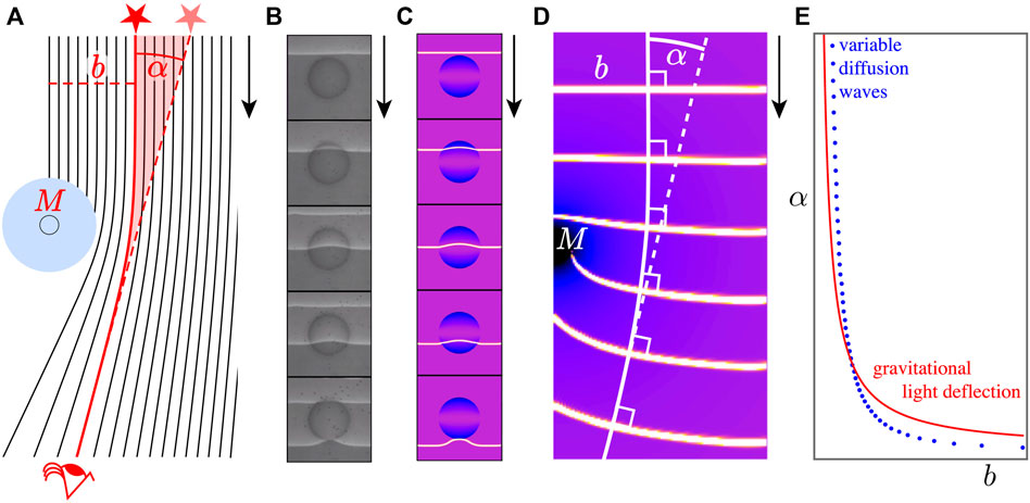
FIGURE 1. Article summary. (A) General relativity predicts the observed gravitational deflection of light near stars with mass M. The deflection angle α depends on the impact parameter b, the perpendicular distance between the initial ray and the star’s center. (B) Experimental reaction-diffusion (RD) over spherical cap obstacles vets our (C) simulated RD over a plane with variable diffusion. (D) Planar RD with variable diffusion can match the effective light speed near a star or black hole and (E) well approximate the famous angle deflection relation α ∝ M/b.

2 General relativity

2.1 Gravitational lensing

Gravitational lensing is an astrophysical general relativity phenomenon that occurs when a massive object (the “lens”) warps spacetime and deviates the path of the light traveling from a distant source to an observer. As a result, the observer may see the apparent position of the real source in a different position, as two or more virtual images, or even as a complete ring if the source, lens, and observer are perfectly aligned. This effect was first described by Albert Einstein in a scratch notebook in 1912 [1] but only published in 1936 [2]. The first mention of the now called “Einstein ring” was published by Orest Chwolson, who described it as a “halo effect” in 1924 [3].

This effect was first investigated during the total solar eclipse of 1919 by two British Expeditions. The Einstein prediction of a 1.75-arcsecond deflection of starlight by the Sun was observed by both expeditions by comparing the apparent location of known stars [4]. It took another 60 years for the first astronomical observation of the lens creating this gravitational effect in 1979 by Walsh, Carswell, and Weymann [5] and another 20 years for the first Einstein ring based on data from the Hubble Space Telescope [6]. One of the most beautiful examples is the lensed quasar HE0435-1223 creating four nearly evenly distributed virtual sources after its light passed the foreground galaxy, as in Figure 2.

FIGURE 2

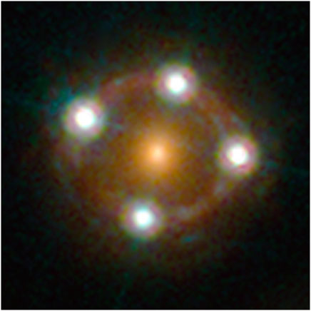
FIGURE 2. Gravitational lensing effect of light from the quasar HE0435-1223 after passing a galaxy. (Credit: ESA/Hubble, NASA, Suyu et al. released under the Creative Commons Attribution 4.0 International license.).

Nowadays, gravitational lensing is used as an astronomical tool to, for example, search for dark energy and dark matter [7], determining mass distributions of distant sources [8], or determining the distance of massive objects such as black holes [9] and quasars [10]. Besides light, gravitational waves can also be influenced by the strong lensing effect of galaxies and clusters and have even been proposed to be used to determine cosmological parameters [11].

2.2 Previous analogs

Because many astronomical phenomena are difficult to imagine, scientists have always been fascinated by lab-size analogs, either to provide a scaled-down, accessible setup for visualization or to find similar phenomena on quite different spatial scales. Johannes Kepler wrote [12],

“And I cherish more than anything else the Analogies, my most trustworthy masters. They know all the secrets of Nature, and they ought to be least neglected in Geometry.”

Many black hole analogs have been created in the past [12, 13]. Gravitational lensing (GL) analogs using scaled-down optical experiments date back as far as 1969 [14]. Since then, various setups have been used to recreate the deformed spacetime around massive objects that bend the path of light rays to visualize the astronomical lensing effect. Those systems include using milled Plexiglas lenses [15–18], transparent photopolymer resin lenses using a stereolithography 3D printer [19], a broken off wine glass base [20, 21], or even a full wine glass [22]. In 2021, Selmke used small disks placed in water for their optical GL analog. The surface tension of the water-air interface raised the menisci around the small discs, creating the necessary curvature for the light to bend [23].

In 2022, Catheline et al. published the first non-optical GL analog which featured surface tension waves moving across a fabric membrane [24]. Their work inspired this project. In their experiment, they stretched different types of fabric over a drum pad and pulled the fabric downwards at one spot to create a warped depression, which is analogous to the gravity well caused by the warping of spacetime around a massive object. Using a ruler and a drumstick, they initiated a planar mechanical surface wave and recorded its propagation with a high-speed camera.

2.3 Weak-field light deflection

Gravitational lensing results from the deflection of light’s path caused by large mass concentrations. As described by Einstein’s general theory of relativity, massive objects distort spacetime around them, changing the trajectory of light.

The nature of light has been questioned by scientists throughout history [25], including a big debate over its composition in the 18th century. In 1704, Isaac Newton argued that light was no exception to his laws of classical mechanics [26]. He proposed that light was composed of particles that experience gravitational pulls from other bodies. This theory contradicted the theory championed by Christiaan Huygens a century earlier, which stated that light propagated as a wave through a physical medium called the “ether” [27]. Many scientists were more inclined towards Huygens’ theory because of the experiments conducted by Augustin-Jean Fresnel on light interference and diffraction in 1819.

But already in 1783, John Michell predicted the existence of “dark stars” (or black holes) by treating light as particles, and in a 1784 letter to Henry Cavendish he hypothesized that one could estimate a star’s mass by measuring how the speed of its light would slow due to its gravitational pull [28]. Likely inspired by this letter, Cavendish used purely classical mechanics to estimate a light ray’s angle of deflection α₀ from a mass M depending on the distance of closest approach d as

${\alpha }_0=\frac{2GM}{c^{2}d},(1)$

with G as the gravitational constant and c as the speed of light. The light ray from the original light source passes an object at a distance d and experiences a deflection of angle α₀, so from the observer’s perspective, the light ray appears to have come from a different direction, creating an apparent source position. The true deflection angle α = 2α₀ is shown in Figure 1A.

Because the wave-nature of light was established in favor of the ether theory, the idea that gravity could affect light was not considered to be accurate throughout the 19th century. It was not until Albert Einstein formulated his “Principle of Equivalence” that the debate was open again. He stated that gravitational mass and inertial mass were indistinguishable from each other. It follows that light, though being massless, had to experience the effects of gravity as well and would change its trajectory when passing a massive object, due to its gravitational effect.

Einstein published his calculation of the deflection angle α₀ in 1911 [29] based on his “Theory of Special Relativity” and the calculations agreed with Cavendish’s Eq. 1 result. In November 1915, Einstein submitted four papers to the Prussian Academy of Sciences about aspects of the “Theory of General Relativity” in which he explained that Newtonian mechanics was not a perfect description of how bodies behaved on a bigger scale. His revolutionary gravitational theory proposed that matter curves spacetime and other particles move along the corresponding spacetime geodesics. A cumulative 54-page article was published 1 year later [30] (see also the review article [31]). Einstein recalculated the correct weak-field deflection angle to be

$\alpha =\frac{4GM}{c^{2}b}=\frac{2R_{\text{s}}}{b}=\frac{2}{b/R_{\text{s}}},(2)$

where R _s = 2GM/c² is the deflector’s Schwarzschild radius, and b is the light ray’s impact parameter, the perpendicular distance between the initial ray and the gravitational source. This is surprisingly similar to Eq. 1, just off by a factor of 2 (although by dimensional analysis, it must be similar). Indeed, half the deflection is due to special relativistic “slow time,” and half is due to general relativistic “space warp.”

In 1919, Arthur Eddington considered Einstein’s prediction and helped organize an experiment to confirm it by recording the positions of stars that appeared closest to the Sun during an eclipse (when they could be seen in daylight) compared to the same stars in the nighttime sky without the Sun [32]. The stars appeared to shift position by angles consistent with the 1.75 arc seconds predicted by Eq. 2 and not by Eq. 1.

3 Physical obstacle experiment

3.1 Reaction-diffusion system

Reaction-diffusion (RD) systems are responsible for many self-organizing phenomena in nature [33, 34] and the chemical Belousov-Zhabotinsky reaction [35, 36] has been used since the 1970s to explore the behavior of temporarily oscillating systems, spatially frozen Turing patterns, and propagating spatio-temporal excitation waves.

In a quasi-two-dimensional, excitable Belousov-Zhabotinsky (BZ) system, waves propagate due to spatio-temporal concentration changes of their chemical components and the resulting diffusion effects. The oxidation and reduction of the catalyst, which also acts as a color indicator, creates visible oxidation waves in the reduced background solution.

The reaction-diffusion system chosen to model the gravitational lensing effect was BZ waves because of the color contrast between the wavefronts and the rest of the reaction. The visibility of their waves makes the study of BZ wave propagation easy to conduct. Their chemical composition has been perfected throughout the years to produce a wavefront propagating system that can be easily visualized by the human eye and therefore measured accurately.

The experimental setup consisted of a monochrome charge-coupled-device (CCD) camera (Basler acA2000-50 gm, 2048 pixel × 1088 pixel) and a frosted glass pane, to make the light from the backlight below as homogeneous as possible, and to hold the acrylic mold with the BZ system. We placed a blue filter between the mold and the camera to increase the contrast in the absorption spectra between the oxidized, blue waves and the reduced, red background. Images were saved every second with a self-designed LabVIEW program which controls the frame grabber card (National Instruments PCIe-8236) and saved on a computer for further processing using the open-source NIH sponsored software Fiji [37].

3.2 Acrylic glass mold

We used an acrylic glass mold with various obstacles, creating a hollow, quasi-two-dimensional system with a constant thickness of 0.5 mm in the normal direction, as in Figure 3. The mold contained thirteen obstacles: two hemispherical shells, which were not used in our experiment, and eleven spherical cap shells with radii R between 3.00 mm and 13.00 mm and heights h = 2.00 mm. The BZ solution was poured into the negatively curved dips in the mold bottom, on the right of Figure 3A, before the mold top, on the left of Figure 3A, was placed onto it to create the quasi-two-dimensional system. Figure 3B is a side image of a filled system with clearly visible obstacles. The filled planar part of the system is not visible.

FIGURE 3

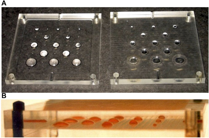
FIGURE 3. (A) Oblique view of pieces of the acrylic glass mold with various spherical cuts within a planar region. (B) Nearly side view of closed mold with BZ solution, creating a hollow space with constant thickness. The inside area is (75 × 75) mm² (from [38]).

To understand the effect of each obstacle on a propagating wave, one needs to determine the path length difference between the planar path d_p (just passing the obstacle) and the curved path d_c across the center line of the obstacle. Figure 4 is a side view sketch of a spherical cap shell. The quasi-two-dimensional BZ solution is placed in the 0.50 mm gap between the two mold sides. All values are based on the center line of the gap. For each obstacle, radius R and cap height h create a spherical cap with base radius r. From the geometry, the cap’s base radius $r=\sqrt{h(2R-h)}$, and the contact angle (between the normal to the sphere at the cap bottom and the base plane) α = arcsin[(R − h)/R]. The planar path length d_p = 2r, and the curved path length

$d_{\text{c}}=R\theta =R\left(\pi -2\alpha \right)=R\hspace{0.17em}\left(\pi -2\arcsin \left[\frac{R-h}{h}\right]\right).(3)$

This path length difference between the outside and the obstacle is the reason for the deformation of the initially straight wavefront. The front section moving over the obstacle experiences a longer path length, resulting in a delayed exit compared to the planar front sections on either side. This delay is largest for the front section moving exactly across the top of the spherical cap (passing through the point at cap height h in Figure 4) and decreases to zero when reaching the planar region around the obstacle.

FIGURE 4

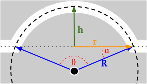
FIGURE 4. Side view drawing of a spherical cap shell with its defining parameters radius R and cut height h. The cap’s base circle r, the total obstacle angle θ, and the contact angle α are necessary to derive the path length across an obstacle.

3.3 Belousov-Zhabotinsky reaction

The Belousov-Zhabotinsky (BZ) reaction is complicated with many intermediate steps [39], but the overall ferroin-catalyzed malonic acid BZ reaction can be summarized as

$\text{malonic\hspace{0.17em}acid}+\text{bromate}\underset{\text{sulfuric\hspace{0.17em}acid}}{\overset{\text{ferroin}}{\to }}\text{bromine}+\text{carbon\hspace{0.17em}dioxide}+\text{water}.(4)$

We used initial concentrations of 0.04 M for malonic acid and for sodium bromate. The 1.2 mM sodium dodecyl sulfate (SDS) addition decreased the BZ solution’s surface tension to suppress the creation of larger carbon dioxide bubbles that might otherwise interfere with the propagating wavefronts. The stock solutions of malonic acid (Alfa Aesar), sodium bromate (Fluka), and SDS (Amresco) were prepared in nanopure water of resistivity 18.2 MΩ m (Barnstead D11931). 4.0 mM ferroin from a ThermoScientific 25 mM stock solution catalyzed the reaction and acted as a redox color indicator. 0.20 M sulfuric acid from a Ricca Chemical Company 1 M stock solution provided protons for the intermediate reactions.

3.4 Experimental results

Two exemplary passing of waves across the obstacles with R = 6 mm and R = 12 mm are shown in Figure 5. Obstacles gently deflect the wavefronts.

FIGURE 5

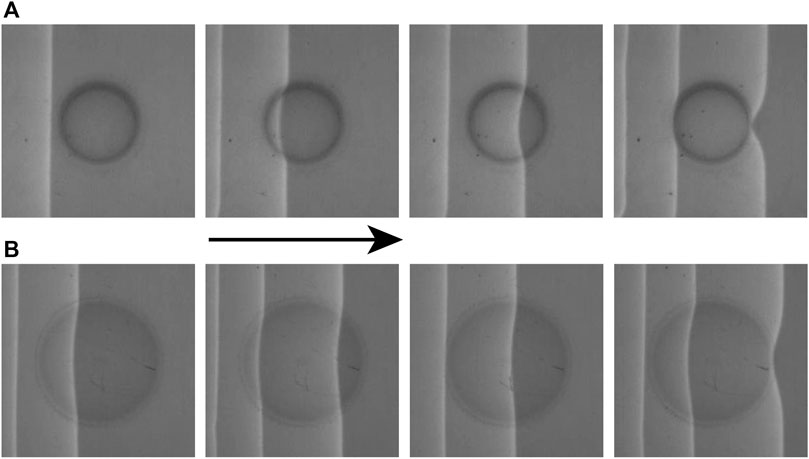
FIGURE 5. Top view of time-series of waves moving across two different Figure 3 spherical caps. (A) Cap has radius R = 6 mm and image has area (14 × 14) mm². (B) Cap has radius R = 12 mm and image has area (16 × 16) mm². Time between images in each series is Δt = 100 s.

4 Diffusive obstacles simulation

4.1 Implementing the Barkley model

To proceed further, we used computer simulations. RD waves in two-dimensional BZ reactions have been modeled successfully for many decades using a variety of computational models. We used the Barkley Model [40] because it was designed to efficiently simulate waves in excitable media.

The Barkley Model is a two-variable reaction-diffusion system where the local kinetics of the reaction are described by

$\frac{\partial u}{\partial t}=f\left(u,v\right)+D{\nabla }^{2}u,(\mathrm{5a})$

$\frac{\partial v}{\partial t}=g\left(u,v\right),(\mathrm{5b})$

where f(u, v) and g(u, v) express the local kinetics of the activator u and the inhibitor v respectively. The parameter D represents the activator diffusion. As there is no diffusion component for the inhibitor, the model assumes an immobilized inhibitor, for example, with BZ solution embedded in a gel matrix [41].

Both the activator and the inhibitor parameters are determined for each point in space within the simulation space. The model sets the functions f(u, v) and g(u, v) to be

$f\left(u,v\right)=\frac{u\left(1-u\right)}{a_1}\left(u-\frac{v+a_2}{a_3}\right),(\mathrm{6a})$

$g\left(u,v\right)=u-v,(\mathrm{6b})$

where the chemical parameters a₁ = 0.005, a₂ = 0.01, and a₃ = 0.3. These two equations define the nonlinear dynamics of the chemical reaction in the absence of diffusion.

Later, for the gravitational analog, we will need variable diffusion D(x, y), so we modify Eq. 5 by replacing the Laplacian term D ∇²u with

$\nabla \cdot J_u=\nabla \cdot \left(D\nabla u\right)=D{\nabla }^{2}u+\nabla D\cdot \nabla u(7)$

according to Fick’s laws of diffusion, where the extra term is small because our diffusion will vary slowly. We will not need the curved-space Laplace-Beltrami operator [42] when we compare experimental RD wavefronts passing over a spherical cap with simulated RD wavefronts passing through a planar variable-diffusion disk.

The activator diffusion represented by the Laplacian ∇²u at any point (x, y) can be computationally approximated on a square grid using the activator variables of neighboring grid points. We first tried a five-point finite-difference Laplacian stencil consisting of the point and its four nearest neighbors. In practice, we found that the five-point formula did not reproduce accurate wavefront curvatures when propagating over our length scales, as shown in Figure 6. So, we upgraded to a skewed nine-point finite-difference stencil consisting of the point and its eight nearest neighbors, including the four nearest diagonal neighbors. The Laplacian approximation became

$\begin{array}{ll}\hfill {\nabla }^2{u}_{i,j}& =u_{i+1,j+1}+u_{i-1,j+1}+u_{i+1,j-1}+u_{i-1,j-1}\hfill \\ \hfill & +4u_{i+1,j}+4u_{i-1,j}+4u_{i,j+1}+4u_{i,j-1}\hfill \\ \hfill & -20u_{i,j}.\hfill \end{array}(8)$

Similarly, we use a central difference approximation for the gradients, including

$\nabla u_{i,j}=\left(\frac{u_{i+1,j}-u_{i-1,j}}{2},\frac{u_{i,j+1}-u_{i,j-1}}{2}\right).(9)$

FIGURE 6

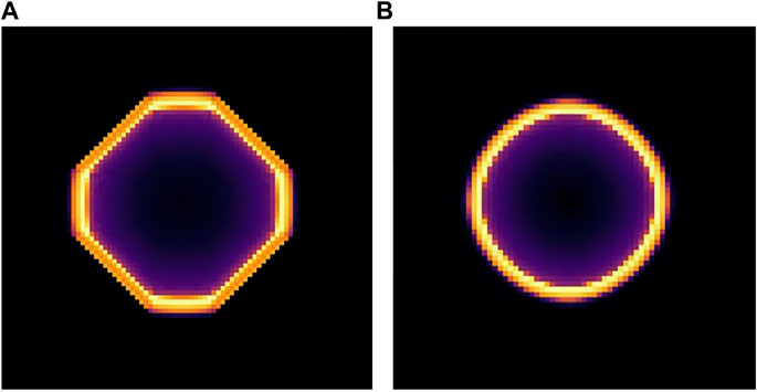
FIGURE 6. Snapshot of a Barkley model simulation of a BZ reaction wave starting from a centered point source using a numerical (A) five-point stencil and a (B) nine-point stencil. Only the latter reproduces the expected circular symmetry. Brighter colors indicate a higher activator concentration.

We created a Python simulation, where a N × N grid simulates a reaction of size N, evaluating Eq. 5 for each point of the grid for every time step. The Barkley model [40] has a simple setup with an efficient algorithm to simulate reaction-diffusion waves. Its evolution steps are simple and accurately model BZ reactions. Modifications to this model can be made in multiple different aspects, such as changing the coefficient of diffusion, adding inhibitor diffusion, or adding obstacles.

4.2 Creating obstacles via diffusion

Diffusion is the way the activator propagates through the reaction resembling a wavefront [43, 44]. The diffusion parameter D, which is constant in time but possibly variable in space, determines how fast the reaction propagates. Just as the fluid drag on a falling object can vary as different powers of its speed, depending on the experiment, so too can the diffusion. In our computer simulations, we find the wave speed increases like the square root of the diffusion parameter, in agreement with other work [45, 46]. This square root relationship was first described by Luther in 1906 for the propagation front of a permanganate/oxalate reaction [47]. Hence, we assume the proportionality

$v\propto \sqrt{D},(10)$

which established the equality

$\frac{v}{c}=\sqrt{\frac{D}{D_u}},(11)$

where c is the maximum speed, and D_u is the maximum diffusion. We denote the maximum diffusion by D_u since it is the initial diffusion chosen for the activator u (and recall that the Barkley inhibitor v does not have a diffusion coefficient since the inhibitor does not propagate).

The diffusion used in the simulation reaction-diffusion space will depend on the obstacles to be modeled, with 0 ≤ D ≤ D_u. With no obstacles, the diffusion is constant across the simulated space. Once the obstacles are defined as speed functions, Eq. 11 yields the equivalent diffusion function.

To simulate Section 3 physical obstacles, the evaluation had to take into account the difference in path lengths within the obstacle regions. Because the simulation is two-dimensional, as if the obstacles were viewed from above, the obstacle regions are circular. In these areas, the wave should slow as if the path lengths increased according to the geometry of the simulated obstacles.

When encountering diffusion obstacles, the activator reduces its propagation speed, which delays its wavefront. If the inhibitor could also diffuse, the inhibitor from the “tail” of the wave might propagate faster than the activator in the wavefront and thereby suppress the wave. This is one reason why no diffusion term was added to the inhibitor rate Eq. 5b. Another reason is that we know of no natural light phenomena resembling a wave inhibitor overrunning its wavefront. Thus, we model light by reaction-diffusion wavefronts with a diffusive activator and a fixed inhibitor.

This model is an approximation but reproduces the behavior observed in the acrylic mold. Converting physical obstacles to diffusion obstacles allows us to extend our reaction-diffusion work from experimentation to simulation.

4.3 Simulation versus experiment

Based on the geometry of Figure 4, we created a diffusion obstacle by systematically decreasing the diffusion parameter where the obstacles would have caused the wavefront to travel vertically, thereby slowing its horizontal motion. Figure 7 compares simulation and experiment. The magenta-to-blue palette codes the diffusion parameter D from higher to lower. The agreement is excellent as the spatially variable diffusion nicely mimics the physical obstacles.

FIGURE 7

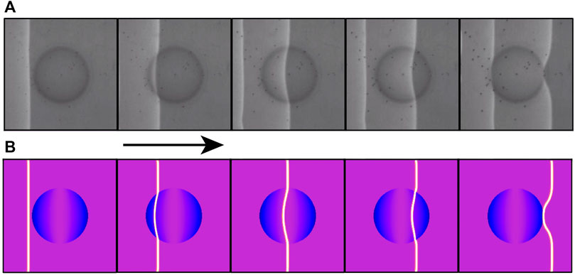
FIGURE 7. (A) Experimental wave propagation through physical obstacles (R = 4 mm, h = 2 mm) and (B) simulated wave propagation with variable diffusion obstacles.

5 Mimicking light deflection

5.1 Effective light speed

To mimic light deflection by a star of mass M with variable diffusion chemistry, we need to determine the effective speed of light in the corresponding spacetime. The pseudo-Euclidean Minkowski line element

$d{s}^2=-c^{2}d{t}^2+d{x}^2+d{y}^2+d{z}^2=-{\left(cdt\right)}^2+d{r}^2(12)$

determines the invariant interval between nearby events in flat spacetime. The perturbed line element

$d{s}^2\approx -\left(1-\frac{R_{\text{s}}}{r}\right){\left(cdt\right)}^2+\left(1+\frac{R_{\text{s}}}{r}\right)d{r}^2(13)$

can incorporate the weak gravity of a mass M, where R _s = 2GM/c² ≪ r is the corresponding Schwarzschild radius [48]. Since light travels along null geodesics, the spacetime interval ds² = 0, and the effective speed

$\frac{v}{c}=\left|\frac{dr}{cdt}\right|\approx {\left(\frac{1-R_{\text{s}}/r}{1+R_{\text{s}}/r}\right)}^{1/2}\sim {\left(1-\frac{2R_{\text{s}}}{r}\right)}^{1/2}\sim 1-\frac{R_{\text{s}}}{r}<1.(14)$

(The rate of change of the r coordinate with respect to the t coordinate is less than c, but the rate of change of proper distance with respect to proper time remains c for all observers.) The corresponding effective refractive index [49, 50] is

$n=\frac{c}{v}\approx {\left(\frac{1+R_{\text{s}}/r}{1-R_{\text{s}}/r}\right)}^{1/2}\sim 1+\frac{R_{\text{s}}}{r}>1.(15)$

Combining Eqs 11, 14, the gives diffusion

$D\sim \left(1-\frac{2R_{\text{s}}}{r}\right)D_u.(16)$

Nearby and in the wake of an obstacle, reaction-diffusion wavefronts behave very differently than light-ray wavefronts deflected by a star, as in Figure 8, but with Eq. 16 variable diffusion, they can elsewhere approximate gravitational light deflection to first order in R_s/r [50].

FIGURE 8

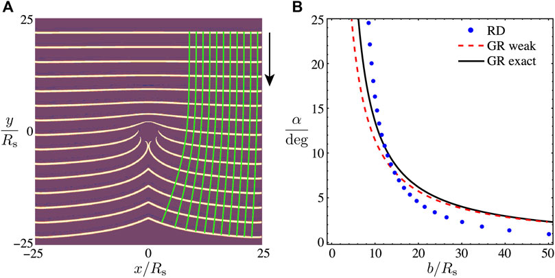
FIGURE 8. From chemical wavefronts to gravitational light deflection. (A) Away from the obstacle center and wake, near-field variable-diffusion wavefronts are well fit by single branches of hyperbolas, asymptotically approaching horizontal far from the center, from which we construct normal rays (green curves). (B) From the starts and ends of the rays, we compute deflection angle α versus impact parameter b (blue dots), which well-approximates the “exact” solution, obtained from the general relativity field and geodesic equations by numerical integration (solid black curve), and its weak-field asymptote, the Einstein deflection Eq. 2 (red dashed curve). A schematic version of this plot appears in Figure 1 summary.

5.2 Light deflection results

Using the resulting diffusion obstacle, we numerically evolve the RD wavefronts forward in time and measure the deflections of the corresponding orthogonal rays. Figure 1D highlights the geometry, including the relation among impact parameter b, deflection angle α, and mass M ∝ R_s.

Figure 8A shows our Python-simulation variable-diffusion wavefronts bending toward the source center. Using Mathematica, we find that translated and scaled hyperbolas y = δy + s/(x − δx), asymptotically approaching horizontal far from the center, well fit the wavefronts, and we use them to construct the normal rays (green curves). The starts of the rays give the impact parameters b and the slopes of the ends of the rays give the deflection angles α. Figure 8B shows that a plot of α versus b (blue dots) is a good approximation both to the weak-field deflection Eq. 2 (red dashed curve) and numerical general relativity (solid black curve), even this close to the source. For comparison, the Sun’s radius is about 240,000 R_s, which is why Eddington and colleagues had to work so hard to first measure gravitational light deflection.

The underlying reaction-diffusion is simulated on an N × N grid as described above, making the simulation run in Θ(N³) time, meaning typical run times are proportional to N³. Each of the N² grid points is updated in each evolution step that propagates the wave forward. The number of steps it takes to propagate the wave to the end of the reaction space is proportional to N. In other words, 100 trials of size N = 100 take approximately 10 min, whereas it takes over 80 h to do the same experiment using N = 1000. Computation time decreases dramatically when running multiple simulations in parallel. Indeed, multiple concurrent simulations of variable-diffusion reaction-diffusion waves with these numerical methods enable us to reproduce the relativistic behavior of gravitational lensing.

6 Discussion

We have proposed a novel analog for general relativistic light deflection, where chemistry elucidates astronomy, and demonstrated its efficacy in a computer simulation vetted by a physical experiment. Remarkably, weak-field gravitational lensing can be described by a variable index of refraction, which defines a variable effective wave speed, which can be engineered into reaction-diffusion waves in systems of variable reaction or diffusion.

The technique of using chemical physics to visualize diverse dynamical systems is very flexible and might have wide applications. Future work is to realize gel-enabled variable diffusion [51, 52] in this and other experiments to mimic a broad range of phenomena. An alternative to gel would be the use of light-sensitive BZ systems [53], whose reaction rate can be controlled with external illumination. Other alternatives could be the use of an electric field [54] to manipulate the diffusion of the inhibitor species or a temperature gradient [55], which can vary both the chemical reaction rate and the diffusion simultaneously. A simple alternative would be to use solid obstacles, which the RD waves would need to propagate around [56, 57]. What other general relativistic phenomena can this technique approximate?

Data availability statement

The raw data supporting the conclusion of this article will be made available by the authors, without undue reservation.

Author contributions

DC-C: Conceptualization, Data curation, Formal Analysis, Investigation, Methodology, Software, Visualization, Writing–original draft, Writing–review and editing. KS: Investigation, Visualization, Writing–review and editing. LD: Supervision, Validation, Writing–review and editing. HG: Formal Analysis, Methodology, Software, Supervision, Writing–review and editing. CL: Formal Analysis, Supervision, Validation, Writing–review and editing. JL: Validation, Visualization, Writing–review and editing. NM: Conceptualization, Data curation, Funding acquisition, Project administration, Supervision, Writing–original draft, Writing–review and editing.

Funding

The author(s) declare financial support was received for the research, authorship, and/or publication of this article. This work was supported by the National Science Foundation (NSF grant DMR-1852095), the Koontz Endowed Fund, and The College of Wooster.

Conflict of interest

The authors declare that the research was conducted in the absence of any commercial or financial relationships that could be construed as a potential conflict of interest.

Publisher’s note

All claims expressed in this article are solely those of the authors and do not necessarily represent those of their affiliated organizations, or those of the publisher, the editors and the reviewers. Any product that may be evaluated in this article, or claim that may be made by its manufacturer, is not guaranteed or endorsed by the publisher.

References

1. Sauer T. Nova Geminorum 1912 and the origin of the idea of gravitational lensing. Archive Hist Exact Sci (2008) 62:1–22. doi:10.1007/s00407-007-0008-4

CrossRef Full Text | Google Scholar

2. Einstein A. Lens-like action of a star by the deviation of light in the gravitational field. Science (1936) 84:506–7. doi:10.1126/science.84.2188.506

PubMed Abstract | CrossRef Full Text | Google Scholar

3. Chwolson O. Über eine mögliche form fiktiver doppelsterne (about a possible form of virtual double stars). Astronomische Nachrichten (1924) 221:329–30. doi:10.1002/asna.19242212003

CrossRef Full Text | Google Scholar

4. Eddington AS. The total eclipse of 1919 May 29 and the influence of gravitation on light. The Observatory (1919) 42:119–22.

Google Scholar

5. Walsh D, Carswell RF, Weymann RJ. 0957 + 561 A, B: twin quasistellar objects or gravitational lens? Nature (1979) 279:381–4. doi:10.1038/279381a0

PubMed Abstract | CrossRef Full Text | Google Scholar

6. King LJ, Jackson N, Blandford RD, Bremer MN, Browne IWA, De Bruyn AG, et al. A complete infrared Einstein ring in the gravitational lens system B1938 + 666. Monthly Notices R Astronomical Soc (1998) 295:L41–4. doi:10.1046/j.1365-8711.1998.295241.x

CrossRef Full Text | Google Scholar

7. Ellis RS. Gravitational lensing: a unique probe of dark matter and dark energy. Phil Trans R Soc A: Math Phys Eng Sci (2010) 368:967–87. doi:10.1098/rsta.2009.0209

PubMed Abstract | CrossRef Full Text | Google Scholar

8. Keeton CR. Computational methods for gravitational lensing (2001). arXiv. doi:10.48550/ARXIV.ASTRO-PH/0102340

CrossRef Full Text | Google Scholar

9. Younas A, Jamil M, Bahamonde S, Hussain S. Strong gravitational lensing by Kiselev black hole. Phys Rev D (2015) 92:084042. doi:10.1103/PhysRevD.92.084042

CrossRef Full Text | Google Scholar

10. Huchra J, Gorenstein M, Kent S, Shapiro I, Smith G, Horine E, et al. 2237 + 0305 - a new and unusual gravitational lens. Astronomical J (1985) 90:691–6. doi:10.1086/113777

CrossRef Full Text | Google Scholar

11. Jana S, Kapadia SJ, Venumadhav T, Ajith P. Cosmography using strongly lensed gravitational waves from binary black holes. Phys Rev Lett (2023) 130:261401. doi:10.1103/PhysRevLett.130.261401

PubMed Abstract | CrossRef Full Text | Google Scholar

12. Barceló C, Liberati S, Visser M. Analogue gravity. Living Rev Relativity (2011) 14:3. doi:10.12942/lrr-2011-3

CrossRef Full Text | Google Scholar

13. Novello M, Visser M, Volovik G. Artificial black holes. World Scientific (2002). doi:10.1142/4861

CrossRef Full Text | Google Scholar

14. Liebes S. Gravitational lens simulator. Am J Phys (1969) 37:103–4. doi:10.1119/1.1975345

CrossRef Full Text | Google Scholar

15. Icke V. Construction of a gravitational lens. Am J Phys (1980) 48:883–6. doi:10.1119/1.12284

CrossRef Full Text | Google Scholar

16. Higbie J. Gravitational lens. Am J Phys (1981) 49:652–5. doi:10.1119/1.12440

CrossRef Full Text | Google Scholar

17. Higbie J. Galactic lens. Am J Phys (1983) 51:860–1. doi:10.1119/1.13507

CrossRef Full Text | Google Scholar

18. Adler RJ, Barber WC, Redar ME. Gravitational lenses and plastic simulators. Am J Phys (1995) 63:536–41. doi:10.1119/1.17865

CrossRef Full Text | Google Scholar

19. Su J, Wang W, Wang X, Song F. Simulation of the gravitational lensing effect of galactic dark matter halos using 3D printing technology. Phys Teach (2019) 57:590–3. doi:10.1119/1.5135783

CrossRef Full Text | Google Scholar

20. Falbo-Kenkel M, Lohre J. Simple gravitational lens demonstrations. Phys Teach (1996) 34:555–7. doi:10.1119/1.2344566

CrossRef Full Text | Google Scholar

21. Huwe P, Field S. Modern gravitational lens cosmology for introductory physics and astronomy students. Phys Teach (2015) 53:266–70. doi:10.1119/1.4917429

CrossRef Full Text | Google Scholar

22. Ros RM. Gravitational lenses in the classroom. Phys Edu (2008) 43:506–14. doi:10.1088/0031-9120/43/5/007

CrossRef Full Text | Google Scholar

23. Selmke M. An optical n-body gravitational lens analogy. Am J Phys (2021) 89:11–20. doi:10.1119/10.0002117

CrossRef Full Text | Google Scholar

24. Catheline S, Delattre V, Laloy-Borgna G, Faure F, Fink M. Gravitational lens effect revisited through membrane waves. Am J Phys (2022) 90:47–50. doi:10.1119/10.0006612

CrossRef Full Text | Google Scholar

25. Meneghetti M. Introduction to gravitational lensing: with Python examples. In: Lecture notes in physics, 956. Cham: Springer International Publishing (2021). doi:10.1007/978-3-030-73582-1

CrossRef Full Text | Google Scholar

26. Newton I. Opticks: or, A treatise of the reflections, refractions, inflexions and colours of light: also two treatises of the species and magnitude of curvilinear figures (London: printed for Sam. Smith, and Benj. Walford, printers to the royal society, at the prince’s arms in St. Paul’s church-yard) (1704).

Google Scholar

27. Huygens C. Traite de la lumiere. Où sont expliquées les causes de ce qui luy arrive dans la reflexion, and dans la refraction. Et particulierment dans l’etrange refraction du cristal d’Islande, (Treatise on Light: in Which Are Explained the Causes of that Which Occurs in Reflection and Refraction and Particularly in the Strange Refraction of Iceland Crystal) (chez Pierre Vander Aa marchand libraire) (1690).

Google Scholar

28. Michell J. VII. On the means of discovering the distance, magnitude, &c. of the fixed stars, in consequence of the diminution of the velocity of their light, in case such a diminution should be found to take place in any of them, and such other data should be procured from observations, as would be farther necessary for that purpose. Phil Trans R Soc Lond (1784) 74:35–57. By the Rev. John Michell, B.D.F.R.S. In a letter to Henry Cavendish, Esq. F.R.S. and A.S. doi:10.1098/rstl.1784.0008

CrossRef Full Text | Google Scholar

29. Einstein A. Über den Einfluß der Schwerkraft auf die Ausbreitung des Lichtes on the influence of gravitation on the propagation of light. Annalen der Physik (1911) 340:898–908. doi:10.1002/andp.19113401005

CrossRef Full Text | Google Scholar

30. Einstein A. Die Grundlage der allgemeinen Relativitätstheorie the basis of general relativity. Annalen der Physik (1916) 354:769–822. doi:10.1002/andp.19163540702

CrossRef Full Text | Google Scholar

31. Ginoux JM. Albert Einstein and the doubling of the deflection of light. Foundations Sci (2022) 27:829–50. doi:10.1007/s10699-021-09783-4

CrossRef Full Text | Google Scholar

32. Dyson FW, Eddington AS, Davdson C. A determination of the deflection of light by the sun’s gravitational field, from observations made at the total eclipse of May 29, 1919. Philosophical Trans R Soc Lond Ser A (1920) 220:291–333. doi:10.1098/rsta.1920.0009

CrossRef Full Text | Google Scholar

33. Field RJ, Burger M. Oscillations and traveling waves in chemical systems. New York: John Wiley and Sons (1985).

Google Scholar

34. Epstein IR, Pojman JA. An introduction to nonlinear chemical dynamics: oscillations, waves, patterns, and chaos. Topics in physical chemistry. New York: Oxford University Press (1998).

Google Scholar

35. Belousov BP. Periodically acting reaction and its mechanism. Collection Abstr Radiat Med 1958 (1959) 1:145–7.

Google Scholar

36. Zhabotinsky AM. Periodic course of oxidation of malonic acid in solution (Investigation of the kinetics of the reaction of Belousov). Biophysics (Moscow) (1964) 9:329–35.

Google Scholar

37. Schindelin J, Arganda-Carreras I, Frise E, Kaynig V, Longair M, Pietzsch T, et al. Fiji: an open-source platform for biological-image analysis. Nat Methods (2012) 9:676–82. doi:10.1038/nmeth.2019

PubMed Abstract | CrossRef Full Text | Google Scholar

38. Manz N. Untersuchungen chemischer Wellen in der Belousov–Zhabotinsky-Reaktion: räumlich modulierte Systeme und anomale Dispersion (Investigation of chemical waves in the Belousov–Zhabotinsky reaction: spatially modulated systems and anomalous dispersion). Ph.D. thesis. Magdeburg: Otto-von-Guericke-Universität Magdeburg (2002).

Google Scholar

39. Edelson D, Field RJ, Noyes RM. Mechanistic details of the Belousov-Zhabotinskii oscillations. Int J Chem Kinetics (1975) 7:417–32. doi:10.1002/kin.550070309

CrossRef Full Text | Google Scholar

40. Barkley D. A model for fast computer simulation of waves in excitable media. Physica D: Nonlinear Phenomena (1991) 49:61–70. doi:10.1016/0167-2789(91)90194-E

CrossRef Full Text | Google Scholar

41. Yamaguchi T, Kuhnert L, Nagy-Ungvarai Z, Müller SC, Hess B. Gel systems for the Belousov-Zhabotinskii reaction. J Phys Chem (1991) 95:5831–7. doi:10.1021/j100168a024

CrossRef Full Text | Google Scholar

42. McGuire MK, Fuller CA, Lindner JF, Manz N. Geographic tongue as a reaction-diffusion system. Chaos: Interdiscip J Nonlinear Sci (2021) 31:033118. doi:10.1063/5.0020906

CrossRef Full Text | Google Scholar

43. Mori H, Kuramoto Y. Dissipative structures and chaos. Berlin Heidelberg: Springer (1998).

Google Scholar

44. Mikhailov AS, Ertl G. Chemical complexity: self-organization processes in molecular systems. The Frontiers collection. Cham: Springer International Publishing (2017). doi:10.1007/978-3-319-57377-9

CrossRef Full Text | Google Scholar

45. Tilden J. On the velocity of spatial wave propagation in the Belousov reaction. J Chem Phys (1974) 60:3349–50. doi:10.1063/1.1681535

CrossRef Full Text | Google Scholar

46. Showalter K, Tyson JJ. Luther’s 1906 discovery and analysis of chemical waves. J Chem Edu (1987) 64:742. doi:10.1021/ed064p742

CrossRef Full Text | Google Scholar

47. Luther R (1906). Spatial propagation of chemical reactions. Z für Elektrochemie 12 (32), 596–600. doi:10.1002/bbpc.19060123208

CrossRef Full Text | Google Scholar

48. Bartelmann M, Maturi M. Weak gravitational lensing. Scholarpedia (2017) 12:32440. doi:10.4249/scholarpedia.32440

CrossRef Full Text | Google Scholar

49. Evans J, Alsing PM, Giorgetti S, Nandi KK. Matter waves in a gravitational field: an index of refraction for massive particles in general relativity. Am J Phys (2001) 69:1103–10. doi:10.1119/1.1389281

CrossRef Full Text | Google Scholar

50. Brown K. Refractions on relativity. Reflections on relativity (2022). p. 550–9. Available at: https://www.mathpages.com/rr/s8-04/8-04.htm (Accessed 2023 December 8).

Google Scholar

51. Bruna M, Chapman SJ. Diffusion in spatially varying porous media. SIAM J Appl Math (2015) 75:1648–74. doi:10.1137/141001834

CrossRef Full Text | Google Scholar

52. Buskohl PR, Vaia RA. Belousov-Zhabotinsky autonomic hydrogel composites: regulating waves via asymmetry. Sci Adv (2016) 2:e1600813. doi:10.1126/sciadv.1600813

PubMed Abstract | CrossRef Full Text | Google Scholar

53. Gáspár V, Bazsa G, Beck MT. The influence of visible light on the Belousov-Zhabotinskii oscillating reactions applying different catalysts. Z für Physikalische Chem (1983) 264:43–8. doi:10.1515/zpch-1983-26406

CrossRef Full Text | Google Scholar

54. Ševčíková H, Marek M. Chemical waves in electric field. Physica D: Nonlinear Phenomena (1983) 9:140–56. doi:10.1016/0167-2789(83)90296-8

CrossRef Full Text | Google Scholar

55. Yamaguchi T, Müller SC. Front geometries of chemical waves under anisotropic conditions. Physica D: Nonlinear Phenomena (1991) 49:40–6. doi:10.1016/0167-2789(91)90191-B

CrossRef Full Text | Google Scholar

56. Wang C, Tan J, Lou B. Influence of obstacles on the propagation speeds of nonlinear waves driven by curvature. Physica A: Stat Mech its Appl (2015) 425:41–9. doi:10.1016/j.physa.2015.01.046

CrossRef Full Text | Google Scholar

57. Smith NJ, Glaser R, Hui VWH, Lindner JF, Manz N. Disruption and recovery of reaction-diffusion wavefronts colliding with obstacles. Physica A: Stat Mech its Appl (2019) 517:307–20. doi:10.1016/j.physa.2018.11.024

CrossRef Full Text | Google Scholar