Rankine-Hugoniot relations in turbulent shocks

1 Introduction

Collisionless shocks are one of the most ubiquitous phenomena in the plasma universe. In fast collisionless shocks the upstream flow is decelerated and the downstream magnetic field, density, and temperature increase. The relations between the upstream and downstream plasma parameters and the magnetic fields are represented using Rankine-Hugoniot relations (RH) [1, 2]. These relations assume that the upstream and downstream states, both sufficiently far from the shock transition layer, are uniform, that is, all relevant variables converge to their constant values. In most cases the ion and electron pressure are assumed isotropic with the polytropic equation of state in both asymptotic regions [2]. These assumptions are especially typical for astrophysical shocks [3]. In a number of studies the assumption of isotropy was relaxed [4–10] but fluctuations are still assumed to disappear. It has been shown that pre-existing turbulence may affect the plasma parameters [11–18].

In the solar wind turbulence at the scales of interest is typically modest [19, 20], while behind the shock transition, in the downstream region, the level of the turbulence is typically by an order of magnitude higher [21–23]. Very long waves with the period of tens of seconds pass from the foreshock of the Earth bow shock and propagate in the magnetosheath toward the magnetopause [24]. Recent simulations show enhancement of turbulence on transmission through the shock [25–27] and modifications of the shock front itself. In these simulations a pre-existing turbulence was included with amplitudes higher than those observed and wavelengths much smaller than those observed, because of the simulation limitations. The box was not large enough to catch the far downstream state of the plasma and magnetic field. Theoretical studies [22, 28] treated transmission of the turbulence which was decoupled from the mean fields. A step toward theoretical incorporation of turbulence in the shock conditions was done within the Burgers equation for an incompressible fluid without magnetic field [11]. It was shown that the magnetic field in shocks may be amplified due to the large scale (wavelength of 10¹–10² shock widths) upstream density fluctuations [29]. RH with turbulence included were introduced ad hoc by [13], without addressing the magnetic field. Observations at the Earth bow shock reveal presence of substantial downstream magnetic fluctuations well behind the shock transition layer in most shocks. Figure 1 shows the magnetic field magnitude measured by the Magnetospheric Multiscale mission (MMS) [30], probe 1, around the shock crossing on 2015-10-21 at 07:05:05 UTC. MMS1 shock crossings are documented on the SHARP webpage https://sharp.fmi.fi/shock-database/ (see also [31]). According to the SHARP list, the angle between the model shock normal [32] and the upstream magnetic field is θ_u = 30° and the Alfvénic Mach number (see definition in Section 4) is M = 9.4. The shown downstream region, t < 0, lasts for 20 min behind the transition at t = 0, while the magnetic field does not converge to a uniform value. These fluctuations have to be taken into account when deriving Rankine-Hugoniot relations. Recently, observed fluctuations of electric and magnetic fields were included in the Poynting flux [33]. In this paper we systematically study Rankine-Hugoniot relations in the presence of a substantial turbulence.

FIGURE 1

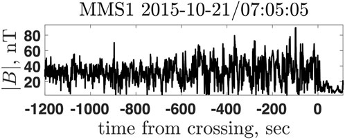
FIGURE 1. The magnetic field magnitude measured by the Magnetospheric Multiscale mission (MMS), probe 1. Large amplitude magnetic fluctuations in the downstream region, t < 0, are clearly seen.

2 General Rankine-Hugoniot relations

We treat the plasma within the magnetohydrodynamic (MHD) approach. The plasma is described by the mass density ρ(x, y, z, t), hydrodynamic velocity V(x, y, z, t), and kinetic pressure P(x, y, z, t). Here we restrict ourselves with the isotropic pressure only. This should be completed with the magnetic field B(x, y, z, t) and electric field E(x, y, z, t). The latter obeys the Ohm’s law E + V ×B/c = 0 in the ideal MHD. The MHD equations for the plasma can be written in the form of conservation laws:

$\frac{\partial }{\partial t}\rho +\frac{\partial }{\partial x_i}{J}_i=0(1)$

$\frac{\partial }{\partial t}\left(\rho V_i\right)+\frac{\partial }{\partial x_j}{T}_{ij}=0(2)$

$\frac{\partial }{\partial t}\left(\frac{1}{2}\rho V^2+ϵ\right)+\frac{\partial }{\partial x_i}{Q}_i=0(3)$

where i = x, y, z, ϵ is the internal energy density, and the mass, momentum, and energy fluxes are

$J_i=\rho V_i(4)$

$T_{ij}=\rho V_i{V}_j+p{\delta }_{ij}+\frac{B^2}{8\pi }{\delta }_{ij}-\frac{B_i{B}_j}{4\pi }(5)$

$Q_i=\left(\frac{1}{2}\rho V^2+ϵ+P\right)V_i+\frac{B^2{V}_i}{4\pi }-\frac{B_i\left(B_j{V}_j\right)}{4\pi }(6)$

These equations are completed with the Maxwell equation

$\frac{\partial }{\partial t}{B}_i=\frac{\partial }{\partial x_j}\left(V_i{B}_j-V_j{B}_i\right)(7)$

Let the shock normal be in the x-direction. This means that after averaging over physically meaningful time and space the x-component of the fluxes are constant

$⟨\rho V_x⟩=⟨J_x⟩=\text{const}(8)$

$⟨\rho V_i{V}_x⟩+⟨P⟩{\delta }_{ix}+⟨\frac{B^2}{8\pi }⟩{\delta }_{ix}-⟨\frac{B_i{B}_x}{4\pi }⟩=⟨T_{ix}⟩=\text{const}(9)$

$\begin{array}{ccc}\hfill & \hfill & ⟨\frac{1}{2}\rho V^2{V}_x⟩+⟨ϵV_x⟩+⟨P{V}_x⟩\hfill \\ \hfill & \hfill & +⟨\frac{B^2{V}_x}{4\pi }⟩-⟨\frac{B_x\left(B_j{V}_j\right)}{4\pi }⟩=⟨Q_x⟩=\text{const}\hfill \end{array}(10)$

and

$⟨V_x{B}_i-V_i{B}_x⟩=0(11)$

We split all variables into a mean part and a fluctuating part using the notation

$\rho \to \rho +r,⟨r⟩=0(12)$

$P\to P+p,⟨p⟩=0(13)$

$ϵ\to ϵ+e,⟨e⟩=0(14)$

$\mathit{V}\to \mathit{V}+\mathit{v},⟨\mathit{v}⟩=0(15)$

$\mathit{B}\to \mathit{B}+\mathit{b},⟨b⟩=0(16)$

Substituting into the fluxes we have

$\rho V_x+⟨r{v}_x⟩=\text{const}(17)$

$\begin{array}{ccc}\hfill & \hfill & \rho V_i{V}_x+P{\delta }_{ix}+\frac{B^2}{8\pi }{\delta }_{ix}-\frac{B_i{B}_x}{4\pi }+\rho ⟨v_i{v}_x⟩\hfill \\ \hfill & \hfill & +⟨r{v}_i⟩V_x+⟨r{v}_x⟩V_i+⟨\frac{b^2}{8\pi }⟩{\delta }_{ix}-⟨\frac{b_i{b}_x}{4\pi }⟩=\text{const}\hfill \end{array}(18)$

$\begin{array}{ccc}\hfill & \hfill & \frac{1}{2}\rho V^2{V}_x+ϵV_x+P{V}_x+\frac{B^2{V}_x}{4\pi }-\frac{B_x\left(B_j{V}_j\right)}{4\pi }\hfill \\ \hfill & \hfill & +⟨r{v}_j⟩V_j{V}_x+\frac{1}{2}⟨r{v}_x⟩V^2+\rho V_x⟨v^2⟩+⟨e{v}_x⟩\hfill \end{array}(19)$

$\begin{array}{ccc}\hfill & \hfill & +⟨p{v}_x⟩+\frac{B_j}{2\pi }⟨b_j{v}_x⟩+\frac{V_x}{4\pi }⟨b^2⟩\hfill \\ \hfill & \hfill & -\frac{B_x}{4\pi }⟨b_j{v}_j⟩-\frac{B_j}{4\pi }⟨b_x{v}_j⟩-\frac{V_j}{4\pi }⟨b_x{b}_j⟩=\text{const}\hfill \\ \hfill & \hfill & V_x{B}_i-V_i{B}_x+⟨v_x{b}_i⟩-⟨v_i{b}_x⟩=0\hfill \end{array}(20)$

$B_x=\text{const}(21)$

In general, triple correlations should be retained and analyzed. For simplicity and brevity in the above expressions only pairwise averages are included. The last equation follows from ∇ ⋅B = 0. A simpler set of equations was proposed by [13] without derivation. The introduced averaging should be an ensemble averaging which is replaced by appropriate time and space averaging (as is done below) for the purposes of the observational data analysis.

3 The case of the shock crossing 2015-10-21/07:05:05

Figure 2 shows three components of the magnetic field in the GSE coordinate system for the MMS1 shock 2015-10-21/07:05:05 mentioned above. In the region −600 < t < − 200 the magnetic field variance exceeds the mean magnetic field squared, ⟨(B −⟨B⟩)²⟩/⟨B⟩² = 2.5. In the region −1200 < t < − 600 the magnetic field variance is smaller but still very significant, ⟨(B −⟨B⟩)²⟩/⟨B⟩² = 0.68. For comparison, Figure 3 shows the ion density, temperature, and speed, calculated onboard by the Fast Plasma Investigation instrument of MMS [34] and Figure 4 shows the electron density, temperature, and speed. The relative fluctuations of these parameters are much smaller, e.g., $⟨{(n_i-⟨n_i⟩)}^2⟩/{(⟨n_i⟩)}^2\approx 0.01$ and $⟨{({\mathit{v}}_i-⟨{\mathit{v}}_i⟩)}^2⟩/{(⟨{\mathit{v}}_i⟩)}^2\approx 0.1$.

FIGURE 2

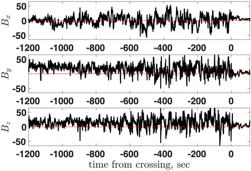
FIGURE 2. The GSE magnetic field components measured by the Magnetospheric Multiscale mission (MMS), probe 1.

FIGURE 3

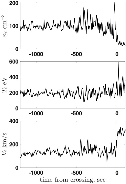
FIGURE 3. Top: the ion density n_i. Middle: the ion temperature T_i. Bottom: the ion speed V_i. All are onboard moments by the FPI instrument [34].

FIGURE 4

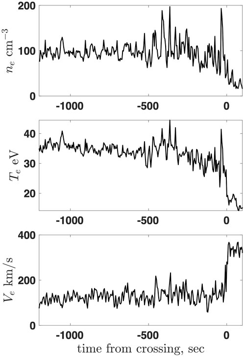
FIGURE 4. Top: the electron density n_e. Middle: the electron temperature T_e. Bottom: the electron speed V_e.

The time resolution for the moments is 4.5 s, much larger than 0.125 s for the magnetic field. However, even quick visual inspection of Figure 2 shows that the temporal scale of the large magnetic fluctuations is comparable with the scale of the density and temperature fluctuations. Thus, the relative significance of the magnetic fluctuations is substantially larger than that of the density and temperature fluctuations.

The ratio of the eigenvalues of the variance matrix S_ij = ⟨b_ib_j⟩ is 1:1.2:1.5, that is, the turbulence is nearly isotropic.

4 Magnetic fluctuations

In view of the above we restrict ourselves here with the magnetic fluctuations only, neglecting r, p, e, and v_i, so that

$\rho V_x=\text{const}(22)$

$\rho V_x^2+P+\frac{B^2}{8\pi }+⟨\frac{b_{\perp }^2}{8\pi }⟩-⟨\frac{b_x^2}{8\pi }⟩=\text{const}(23)$

$\rho V_i{\mathit{V}}_{\perp }-\frac{{\mathit{B}}_{\perp }{B}_x}{4\pi }-⟨\frac{{\mathit{b}}_{\perp }{b}_x}{4\pi }⟩=\text{const},(24)$

$\frac{1}{2}\rho V^2{V}_x+ϵV_x+P{V}_x+\frac{B_x^2{V}_x}{4\pi }+\frac{V_x}{4\pi }⟨b^2⟩=\text{const}(25)$

$V_x{\mathit{B}}_{\perp }-{\mathit{V}}_{\perp }{B}_x=0(26)$

$B_x=\text{const}(27)$

where ⊥ refers to y, z. The case of Alfvén turbulence, where the relative velocity fluctuations are also large and have to be taken into account, has been treated by [35] in the strong shock limit.

Assuming, for simplicity, isotropy of the fluctuations, we have eventually

$\rho V_x=\text{const}(28)$

$\rho V_x^2+P+\frac{B^2}{8\pi }\left(1+\frac{G}{3}\right)=\text{const}(29)$

$\rho V_x{\mathit{V}}_{\perp }-\frac{{\mathit{B}}_{\perp }{B}_x}{4\pi }=\text{const},(30)$

$\begin{array}{ccc}\hfill & \hfill & \frac{1}{2}\rho V^2{V}_x+ϵV_x+P{V}_x\hfill \\ \hfill & \hfill & +\frac{V_x{B}_{\perp }^2-B_x\left({\mathit{V}}_{\perp }\cdot {\mathit{B}}_{\perp }\right)}{4\pi }+\frac{B^{2}G}{4\pi }=\text{const}\hfill \end{array}(31)$

$V_x{\mathit{B}}_{\perp }-{\mathit{V}}_{\perp }{B}_x=\text{const}(32)$

$B_x=\text{const}(33)$

where G = ⟨b²⟩/B².

It is convenient to proceed in the de Hoffman-Teller frame (HT). Let u and d denote upstream and downstream, respectively. Eqs 30, 32 mean that B_u,⊥, B_d,⊥, V_u,⊥, V_d,⊥, and $\widehat{x}$ are all in one plane. Let it be x − z plane. bThe angle between the shock normal and the local magnetic field is given by

$\cos \theta =\frac{B_x}{B}(34)$

$B_u\cos {\theta }_u=B_d\cos {\theta }_d(35)$

for both upstream and downstream. HT is the shock frame in which V_⊥‖B_⊥ in both asymptotic regions. The Normal Incidence Frame (NIF) is the frame in which V_u,⊥ = 0. In NIF ${\mathit{V}}_u=V_u\widehat{x}$ while in HT ${\mathit{V}}_u=U_u{\widehat{B}}_u$, with V_u = U_u cos θ_u and similarly for the downstream region. The Alfvénic Mach number M is defined as

$M=\frac{V_u}{v_A},v_A=\frac{B_u}{\sqrt{4\pi {\rho }_u}}(36)$

It is widely accepted also to define $\beta =8\pi P_u/B_u^2$. With this notation we shall have

${\rho }_u{U}_u\cos {\theta }_u={\rho }_d{U}_d\cos {\theta }_d(37)$

$\begin{array}{ccc}\hfill & \hfill & {\rho }_u{U}_u^2{\cos }^2{\theta }_u+P_u+\frac{B_u^2}{8\pi }\hfill \\ \hfill & \hfill & ={\rho }_d{U}_d^2{\cos }^2{\theta }_d+P_d+\frac{B_d^2}{8\pi }\left(1+\frac{G}{3}\right)\hfill \end{array}(38)$

$\begin{array}{ccc}\hfill & \hfill & {\rho }_u{U}_u^2\sin {\theta }_u\cos {\theta }_u-\frac{B_u^2\sin {\theta }_u\cos {\theta }_u}{4\pi }\hfill \\ \hfill & \hfill & ={\rho }_d{U}_d^2\sin {\theta }_d\cos {\theta }_d-\frac{B_d^2\sin {\theta }_d\cos {\theta }_d}{4\pi }\hfill \end{array}(39)$

$\begin{array}{ccc}\hfill & \hfill & \frac{1}{2}{\rho }_u{U}_u^3\cos {\theta }_u+\left({ϵ}_u+P_u\right)U_u\cos {\theta }_u\hfill \\ \hfill & \hfill & =\frac{1}{2}{\rho }_d{U}_d^3\cos {\theta }_d+\left({ϵ}_d+P_d\right)U_d\cos {\theta }_d+\frac{B_d^{2}G}{4\pi }{U}_d\cos {\theta }_d\hfill \end{array}(40)$

Here we are treating the case where the upstream region is quiet while the downstream region contains significant magnetic fluctuations.

Let us define

$\begin{array}{ccc}\hfill & \hfill & R=\frac{B_d}{B_u},N=\frac{{\rho }_d}{{\rho }_u},\mathrm{\Pi }=\frac{P_d}{{\rho }_u{U}_u^2{\cos }^2{\theta }_u},\hfill \\ \hfill & \hfill & Y=\frac{U_d}{U_u},ϵ+P=\frac{\gamma }{\gamma -1}P\hfill \end{array}(41)$

we have also

$\frac{\cos {\theta }_d}{\cos {\theta }_u}=\frac{B_u}{B_d}=\frac{1}{R}(42)$

Now the equations take the following dimensionless form

$R=NY(43)$

$1+\frac{1+\beta }{2M^2}=\frac{Y}{R}+\mathrm{\Pi }+\frac{R^2\left(1+G/3\right)}{2M^2}(44)$

$1-\frac{{\cos }^2{\theta }_u}{M^2}=\left(Y-\frac{R{\cos }^2{\theta }_u}{M^2}\right)\left(\frac{\sqrt{R^2-{\cos }^2{\theta }_u}}{R\sin {\theta }_u}\right)(45)$

$\begin{array}{ccc}\hfill & \hfill & 1+\frac{\gamma }{\gamma -1}\frac{\beta {\cos }^2{\theta }_u}{M^2}\hfill \\ \hfill & \hfill & =Y^2+\left(\frac{2\gamma \mathrm{\Pi }Y}{R\left(\gamma -1\right)}\right){\cos }^2{\theta }_u+\frac{2RYG{\cos }^2{\theta }_u}{M^2}\hfill \end{array}(46)$

Figure 5 shows the dependence of the density compression N = n_d/n_u (left column) and the magnetic compression R = B_d/B_u (right column) on the Alfvénic Mach number M, for two cases: a) θ_u = 60°, β = 0.2 (top row), and b) θ_u = 20°, β = 2 (bottom row), and for various values of $G=⟨b^2⟩/B_d^2$. In both cases both compression ratios increase with the increase of G. For θ = 60° and sufficiently large G the compression ratios exceed the theoretical maximum for G = 0 and M → ∞. Deviations of the ratios from the standard ratios at G = 0 are larger for lower Mach numbers.

FIGURE 5

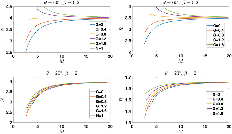
FIGURE 5. The density compression ratio N = n_d/n_u (left column) and the magnetic compression ratio R = B_d/B_u (right column), as functions of the Alfvénic Mach number M, for two cases: a) θ_u = 60°, β = 0.2 (top row), and b) θ_u = 20°, β = 2 (bottom row). In both case presence of fluctuations results in the increase of the compression ratios.

5 Discussion and conclusion

We have shown that undamped fluctuations in the downstream region have to be taken into account in the Rankine-Hugoniot conditions which relate the mean upstream and downstream values of the plasma parameters and magnetic field. It appears that if only isotropic magnetic fluctuations are included, the density and magnetic field compression ratios may be substantially different from those expected from the standard RH. The density compression ratio may even exceed the theoretical maximum for strong shocks. Such unusual density compression ratios are observed at the Earth bow shock. They are usually attributed to the difficulties of particle measurements and are often considered as a sufficient argument to exclude shocks from the analysis [36, 37]. The findings in this paper encourage re-consideration of analysis of shocks with unconventional compression ratios.

The present analysis is incomplete, since we limited ourselves with magnetic fluctuations only. For the shock, used as an example, this was justified, since the relative fluctuations of density and temperature were much smaller. This would not necessarily happen in all shocks, so that other fluctuations have to be taken into account too.

Data availability statement

Publicly available datasets were analyzed in this study. This data can be found here: MMS Science Data Center https://lasp.colorado.edu/mms/sdc/public/.

Author contributions

MG: Conceptualization, Data curation, Formal Analysis, Investigation, Methodology, Validation, Visualization, Writing–original draft, Writing–review and editing.

Funding

The author(s) declare financial support was received for the research, authorship, and/or publication of this article. This study was partially supported by the European Union’s Horizon 2020 research and innovation program under grant agreement No. 101004131 (SHARP) and by the International Space Science Institute (ISSI) in Bern, through ISSI International Team project #23-575.

Acknowledgments

The author is grateful to Steve Schwartz for bringing the paper Schwartz et al. [33] to the author’s attention and thus inspiring this study.

Conflict of interest

The author declares that the research was conducted in the absence of any commercial or financial relationships that could be construed as a potential conflict of interest.

The author(s) declared that they were an editorial board member of Frontiers, at the time of submission. This had no impact on the peer review process and the final decision.

Publisher’s note

All claims expressed in this article are solely those of the authors and do not necessarily represent those of their affiliated organizations, or those of the publisher, the editors and the reviewers. Any product that may be evaluated in this article, or claim that may be made by its manufacturer, is not guaranteed or endorsed by the publisher.

References

1. de Hoffmann F, Teller E. Magneto-hydrodynamic shocks. Phys Rev (1950) 80:692–703. doi:10.1103/PhysRev.80.692

CrossRef Full Text | Google Scholar

2. Kennel CF. Shock structure in classical magnetohydrodynamics. J Geophys Res (1988) 93:8545–57. doi:10.1029/JA093iA08p08545

CrossRef Full Text | Google Scholar

3. McKee CP, Hollenbach DJ. Intestellar shock waves. Ann Rev Astron Astrophys (1980) 18:219–62. doi:10.1146/annurev.aa.18.090180.001251

CrossRef Full Text | Google Scholar

4. Abraham-Shrauner B. Shock jump conditions for an anisotropic plasma. J Plas Phys (1967) 1:379–81. doi:10.1017/S0022377800003366

CrossRef Full Text | Google Scholar

5. Lynn YM. Discontinuities in an anisotropic plasma. Phys Fluids (1967) 10:2278–80. doi:10.1063/1.1762025

CrossRef Full Text | Google Scholar

6. Hudson P. Discontinuities in an anisotropic plasma and their identification in the solar wind. Plan Sp Sci (1970) 18:1611–22. doi:10.1016/0032-0633(70)90036-X

CrossRef Full Text | Google Scholar

7. Lyu LH, Kan JR. Shock jump conditions modified by pressure anisotropy and heat flux for earth’s bowshock. J Geophys Res (1986) 91:6771–5. doi:10.1029/JA091iA06p06771

CrossRef Full Text | Google Scholar

8. Erkaev NV, Vogl DF, Biernat HK. Solution for jump conditions at fast shocks in an anisotropic magnetized plasma. J Plas Phys (2000) 64:561–78. doi:10.1017/S002237780000893X

CrossRef Full Text | Google Scholar

9. Vogl DF, Biernat HK, Erkaev NV, Farrugia CJ, Mühlbachler S. Jump conditions for pressure anisotropy and comparison with the Earth’s bow shock. Nonl Proc Geophys (2001) 8:167–74. doi:10.5194/npg-8-167-2001

CrossRef Full Text | Google Scholar

10. Génot V. Analytical solutions for anisotropic MHD shocks. Astrophys Sp Sci Trans (2009) 5:31–4. doi:10.5194/astra-5-31-2009

CrossRef Full Text | Google Scholar

11. Zank GP, Zhou Y, Matthaeus WH, Rice WKM. The interaction of turbulence with shock waves: a basic model. Phys Fluids (2002) 14:3766–74. doi:10.1063/1.1507772

CrossRef Full Text | Google Scholar

12. Völk HJ, Berezhko EG, Ksenofontov LT. Magnetic field amplification in Tycho and other shell-type supernova remnants. Astron Astrophys (2005) 433:229–40. doi:10.1051/0004-6361:20042015

CrossRef Full Text | Google Scholar

13. Terasawa T, Hada T, Matsukiyo S, Oka M, Bamba A, Yamazaki R. Shock modification by cosmic-ray-excited turbulences. Progr Theor Phys Suppl (2007) 169:146–9. doi:10.1143/PTPS.169.146

CrossRef Full Text | Google Scholar

14. Niemiec J, Pohl M, Stroman T, Nishikawa K-I. Production of magnetic turbulence by cosmic rays drifting upstream of supernova remnant shocks. Astrophys J (2008) 684:1174–89. doi:10.1086/590054

CrossRef Full Text | Google Scholar

15. Adhikari L, Zank GP, Hunana P, Hu Q. The interaction of turbulence with parallel and perpendicular shocks. J Phys Conf Ser (2016) 767:012001. doi:10.1088/1742-6596/767/1/012001

CrossRef Full Text | Google Scholar

16. Guo F, Giacalone J, Zhao L. Shock propagation and associated particle acceleration in the presence of ambient solar-wind turbulence. Front Astron Space Sci (2021) 8:644354. doi:10.3389/fspas.2021.644354

CrossRef Full Text | Google Scholar

17. Nakanotani M, Zank GP, Zhao L-L. Turbulence-dominated shock waves: 2D hybrid kinetic simulations. Astrophys J (2022) 926:109. doi:10.3847/1538-4357/ac4781

CrossRef Full Text | Google Scholar

18. Wang B-B, Zank GP, Zhao L-L, Adhikari L. Turbulent cosmic ray–mediated shocks in the hot ionized interstellar medium. Astrophys J (2022) 932:65. doi:10.3847/1538-4357/ac6ddc

CrossRef Full Text | Google Scholar

19. Sahraoui F, Hadid L, Huang S. Magnetohydrodynamic and kinetic scale turbulence in the near-Earth space plasmas: a (short) biased review. Rev Mod Plasma Phys (2020) 4:4. doi:10.1007/s41614-020-0040-2

CrossRef Full Text | Google Scholar

20. Fraternale F, Adhikari L, Fichtner H, Kim TK, Kleimann J, Oughton S, et al. Turbulence in the outer heliosphere. Sp Sci Rev (2022) 218:50. doi:10.1007/s11214-022-00914-2

CrossRef Full Text | Google Scholar

21. Pitňa A, Šafránková J, Němeček Z, Franci L. Decay of solar wind turbulence behind interplanetary shocks. Astrophys J (2017) 844:51. doi:10.3847/1538-4357/aa7bef

CrossRef Full Text | Google Scholar

22. Zank GP, Nakanotani M, Zhao LL, Du S, Adhikari L, Che H, et al. Flux ropes, turbulence, and collisionless perpendicular shock waves: high plasma beta case. Astrophys J (2021) 913:127. doi:10.3847/1538-4357/abf7c8

CrossRef Full Text | Google Scholar

23. Zhao L-L, Zank GP, He JS, Telloni D, Hu Q, Li G, et al. Turbulence and wave transmission at an ICME-driven shock observed by the Solar Orbiter and Wind. Astron Astrophys (2021) 656:A3. doi:10.1051/0004-6361/202140450

CrossRef Full Text | Google Scholar

24. Turc L, Roberts OW, Verscharen D, Dimmock AP, Kajdič P, Palmroth M, et al. Transmission of foreshock waves through Earth’s bow shock. Nat Phys (2023) 19:78–86. doi:10.1038/s41567-022-01837-z

PubMed Abstract | CrossRef Full Text | Google Scholar

25. Trotta D, Valentini F, Burgess D, Servidio S. Phase space transport in the interaction between shocks and plasma turbulence. PNAS (2021) 118:e2026764118. doi:10.1073/pnas.2026764118

PubMed Abstract | CrossRef Full Text | Google Scholar

26. Trotta D, Pecora F, Settino A, Perrone D, Hietala H, Horbury T, et al. On the transmission of turbulent structures across the earth’s bow shock. Astrophys J (2022) 933:167. doi:10.3847/1538-4357/ac7798

CrossRef Full Text | Google Scholar

27. Trotta D, Pezzi O, Burgess D, Preisser L, Blanco-Cano X, Kajdic P, et al. Three-dimensional modelling of the shock–turbulence interaction. MNRAS (2023) 525:1856–66. doi:10.1093/mnras/stad2384

CrossRef Full Text | Google Scholar

28. Ao X, Zank GP, Pogorelov NV, Shaikh D. Interaction of a thin shock with turbulence. I. Effect on shock structure: analytic model. Phys Fluids (2008) 20. doi:10.1063/1.3041706

CrossRef Full Text | Google Scholar

29. Giacalone J, Jokipii JR. Magnetic field amplification by shocks in turbulent fluids. Astrophys J (2007) 663:L41–4. doi:10.1086/519994

CrossRef Full Text | Google Scholar

30. Russell CT, Anderson BJ, Baumjohann W, Bromund KR, Dearborn D, Fischer D, et al. The magnetospheric Multiscale magnetometers. Space Sci Rev (2016) 199:189–256. doi:10.1007/s11214-014-0057-3

CrossRef Full Text | Google Scholar

31. Lalti A, Khotyaintsev YV, Dimmock AP, Johlander A, Graham DB, Olshevsky V. A database of MMS bow shock crossings compiled using machine learning. J Geophys Res (2022) 127:e2022JA030454. doi:10.1029/2022JA030454

CrossRef Full Text | Google Scholar

32. Farris MH, Russell CT. Determining the standoff distance of the bow shock: Mach number dependence and use of models. J Geophys Res (1994) 99:17681–9. doi:10.1029/94JA01020

CrossRef Full Text | Google Scholar

33. Schwartz SJ, Goodrich KA, Wilson LB, Turner DL, Trattner KJ, Kucharek H, et al. Energy partition at collisionless supercritical quasi-perpendicular shocks. J Geophys Res (2022) 127:e2022JA030637. doi:10.1029/2022JA030637

CrossRef Full Text | Google Scholar

34. Pollock C, Moore T, Jacques A, Burch J, Gliese U, Omoto T, et al. Fast plasma investigation for magnetospheric Multiscale. Space Sci Rev (2016) 199:331–406. doi:10.1007/s11214-016-0245-4

CrossRef Full Text | Google Scholar

35. Gedalin M. Rankine–hugoniot relations and magnetic field enhancement in turbulent shocks. Astrophys J (2023) 958:2. doi:10.3847/1538-4357/ad0461

CrossRef Full Text | Google Scholar

36. Gedalin M, Russell CT, Dimmock AP. Shock Mach number estimates using incomplete measurements. J Geophys Res (2021) 126:e2021JA029519. doi:10.1029/2021JA029519

CrossRef Full Text | Google Scholar

37. Gedalin M, Golan M, Vink J, Ganushkina N, Balikhin M. Electron heating in shocks: statistics and comparison. J Geophys Res (2023) 128:e2023JA031627. doi:10.1029/2023JA031627

CrossRef Full Text | Google Scholar