Generalized connectivity in cubic fuzzy graphs with application in the trade deficit problem
 Yongsheng Rao
 Ruxian Chen1
  Uzma Ahmad
- 1Institute of Computing Science and Technology, Guangzhou University, Guangzhou, China
- 2Department of Mathematics, University of the Punjab, Lahore, Pakistan
Cubic fuzzy graphs (CFGs) offer greater utility as compared to interval-valued fuzzy graphs and fuzzy graphs due to their ability to represent the degree of membership for vertices and edges using both interval and fuzzy number forms. The significance of these concepts motivates us to analyze and interpret intricate networks, enabling more effective decision making and optimization in various domains, including transportation, social networks, trade networks, and communication systems. This paper introduces the concepts of vertex and edge connectivity in CFGs, along with discussions on partial cubic fuzzy cut nodes and partial cubic fuzzy edge cuts, and presents several related results with the help of some examples to enhance understanding. In addition, this paper introduces the idea of partial cubic α-strong and partial cubic δ-weak edges. An example is discussed to explain the motivation behind partial cubic α-strong edges. Moreover, it delves into the introduction of generalized vertex and edge connectivity in CFGs, along with generalized partial cubic fuzzy cut nodes and generalized partial cubic fuzzy edge cuts. Relevant results pertaining to these concepts are also discussed. As an application, the concept of generalized partial cubic fuzzy edge cuts is applied to identify regions that are most affected by trade deficits resulting from street crimes. Finally, the research findings are compared with the existing method to demonstrate their suitability and creativity.
1 Introduction
Graph theory plays a vital role in numerous disciplines, including mathematics, engineering, physical sciences, social sciences, biology, computer science, linguistics, and more. The concept of fuzzy graphs emerges from the recognition that networks can exhibit ambiguity or uncertainty. This constitutes a crucial area of research. Traditional graphs face limitations in adequately capturing the uncertain attributes of network measurements, such as robust connections, accomplished individuals, and influential figures within social networks. In contrast, fuzzy graphs offer a more effective representation of these less-defined aspects. The acknowledgment of uncertainty in specific aspects of graph theory problems has spurred the evolution of fuzzy theory. The concept of fuzzy set (FS) theory, an extension of the classical set notion, was introduced by Zadeh [1] in 1965. Building upon this theory, Zadeh proposed a mathematical approach that enables decision-making problems through the use of fuzzy descriptions. In 1975, Rosenfeld [2] introduced fuzzy graph theory, combining the concepts of FS theory and graph theory. Around the same time, Yeh and Bang [3] also introduced the concept of fuzzy graphs (FGs). FGs find application in various scientific and engineering fields, such as broadcast communications, artificial reasoning, data hypothesis, and neural systems. Akram et al. [4] presented the idea of m-polar fuzzy hypergraphs, m-polar fuzzy line graphs, dual m-polar fuzzy hypergraphs, and 2-section of m-polar fuzzy hypergraphs.
FG theory is a significant and extensive area of research with a primary focus on connectivity. Different fuzzy connectivity measures were discussed in [5–14], 15–19. Mathew and Sunitha [20, 21] examined the concepts of edge connectivity, vertex connectivity, and cycle connectivity in FGs. Banerjee [22] and Tong and Zheng proposed various algorithms for analyzing connectivity in FGs. Ali et al. [23] discussed the notion of t-connected fuzzy graphs and average fuzzy vertex connectivity. Ahmad and Nawaz [24] explored the application of connectivity in directed rough graphs for trade networking. Shang [25] introduced some asymptotic results on r-super connectedness for classical Erdos–Rényi random graphs as the number of nodes tends to infinity. Su et al. [26] presented sufficient conditions in terms of the forgotten topological index for a graph to be l-connected, l-deficient, l-Hamiltonian, and l-independent, respectively. Binu et al. investigated the connectivity index of FGs and its application in the context of human trafficking. Mandal and Pal [27] introduced the concept of the connectivity index of m-polar fuzzy graphs and discussed the boundedness of the connectivity index. Amer et al. [28] calculated the edge-based counterparts of several notable topological degree-based indices, including the Randic index, sum-connectivity index, Zagreb indices, atom–bond connectivity (ABC) index, harmonic index, and geometric–arithmetic (GA) index for Boron triangular nanotubes. Irfan et al. [29] derived closed forms for M-polynomials pertaining to the line graphs of H-naphthalenic nanotubes and chain silicate networks. Using these M-polynomials, various topological indices based on degrees were obtained. The characteristics of fuzzy trees were studied by Sunitha and Vijayakumar [30] in 1999, while Mathew et al. [31] examined the characterization of fuzzy trees and cycles using saturation counts. Mordeson et al. [32] analyzed the properties of different types of fuzzy bridges and fuzzy cut vertices in FGs. Bhutani et al. introduced the concept of strong edges in fuzzy graphs and also discussed fuzzy end nodes in [33]. Talebi et al. [34] presented the idea of weak isomorphism, self-weak complementary, and co-weak isomorphism on vague graphs. Talebi et al. [35] investigated relations among union, join, and complement operations on bipolar fuzzy graphs. Mathew and Sunitha proposed various types of arcs, such as α-strong, β-strong, and δ-edges, in FGs [36]. Karunambigai et al. [37] introduced different types of arcs in intuitionistic FGs. Akram et al. [38] presented the idea of strong edges for m-polar fuzzy graphs in 2021. Naeem et al. [39] proposed the connectivity index for intuitionistic FGs. Last, Binu et al. [40] introduced the concept of the cyclic connectivity index in 2020.
Zadeh [41] proposed interval-valued fuzzy sets (IVFSs) as an extension of FSs, where membership degrees are represented by interval numbers instead of single points. Akram [42] presented the idea of interval-valued fuzzy line graphs and discussed some of their properties. Talebi et al. [43] introduced novel concepts of interval-valued intuitionistic fuzzy graphs (IVIFGs). Talebi et al. [44] introduced the concept of interval-valued intuitionistic fuzzy competition graphs of an interval-valued intuitionistic fuzzy digraph and investigated their properties. Rashmanlou et al. [45] introduced the concept of several types of interval-valued intuitionistic (S, T)-fuzzy graphs and also introduced different kinds of arc interval-valued intuitionistic (S, T)-fuzzy graphs.
In 2012, Jun et al. [46] introduced cubic fuzzy sets (CFSs) as a combination of IVFSs and FSs, offering a more generalized approach for handling uncertainty. They also provided an explanation of basic properties and operations.
Jun et al. [27] further extended the CFS by merging it with the neutrosophic complex, giving rise to the neutrosophic CFS. Cubic fuzzy sets present clear advantages compared to other fuzzy set types, such as interval-valued or general fuzzy sets. Their distinctive shape and parameters offer exceptional flexibility for modeling uncertainty. This flexibility allows for a more precise representation of complex relationships within a specific domain. The enhanced decision-making and reasoning capabilities of cubic fuzzy sets make them invaluable tools in various fields that depend on accurately modeling uncertainty. In 2018, Rashid et al. [47] introduced cubic fuzzy graphs (CFGs) based on CFSs. However, the initial definition of CFGs proposed by Rashid et al. [47] was later found to be incorrect, and a revised definition was provided by Muhiuddin et al. [48] in 2020. Fang et al. [49] discussed the planarity in cubic intuitionistic graphs and also introduced the concept of the degree of planarity in cubic intuitionistic planar graphs. Muhiuddin et al. [50] worked on cubic Pythagorean fuzzy graphs (CPFGs) and introduced certain fundamental operations, such as the lexicographical product, semi-strong product, and symmetric difference of two CPFGs. Muhiuddin et al. [51] discussed the concept of strong and weak edges for cubic planar graphs in 2022. In real-world scenarios, fuzzy graph ideas prove effective in describing certain phenomena, while interval-valued graph concepts excel in others. However, for more intricate phenomena that cannot be adequately represented by either of these approaches alone, a combination of both becomes valuable, referred to as cubic fuzzy graphs. An example illustrating the utility of this combined modeling approach is in addressing the trade deficit problem. When decisions require consideration of the past, present, and future simultaneously, cubic fuzzy graphs prove quite advantageous. They serve as a valuable tool for visually representing information spanning multiple time dimensions, offering a comprehensive view of the situation at hand.
1.1 Motivation and contribution
CFGs offer a more advantageous representation by integrating the membership degree of vertices and edges in both interval and fuzzy number forms. This enhanced representation fosters a more profound and detailed understanding of the connections and uncertainties inherent in the graph’s structure. The following features of edge cuts and cut nodes in CFG theory serve as the motivation for presenting this paper:
• While FGs or IVFGs may suffice for resolving certain practical problems, more intricate issues often demand a fusion of both. CFGs present a valuable approach for tackling such complex problems. Examples encompass traffic flow modeling, trade deficit modeling, and earthquake modeling, where CFGs can offer insightful perspectives.
• The motivation behind our research stems from the fact that the concepts of edge cuts and cut nodes have been well documented in the literature for crisp and fuzzy graphs, and their counterparts in CFGs are not widely known. Investigating their relevance and implications in the context of CFGs is, therefore, a worthwhile endeavor.
• The analysis of edge cuts and cut nodes holds significant potential in various decision-making problems, offering valuable insights and aiding in informed decision-making processes.
This paper introduces the notions of partial cubic fuzzy edge cuts, partial cubic fuzzy cut nodes, generalized partial cubic fuzzy edge cuts, and generalized partial cubic fuzzy cut nodes for CFGs. It builds upon the substantial significance and wide-ranging applications of edge cuts and cut nodes in fuzzy networks. Generalized partial cubic fuzzy edge cuts are particularly advantageous in addressing practical issues where the concept of fuzzy edge cuts may not be applicable. In particular, these concepts become relevant when the IVF-connectivity experiences a strict decrease upon the removal of a specific edge or any edge, while the F-connectivity remains equivalent to the F-connectivity of an edge after its removal or the removal of any specific edge and vice versa. In scenarios where we have information about the past, future, and current conditions of a model or problem, we can represent the past condition as a lower IVF-membership, the future condition as an upper IVF-membership, and the present condition as an F-membership value. Our objective is to scrutinize the problem by deducing lower IVF-connectivity, upper IVF-connectivity, and F-connectivity. Furthermore, we aim to make new predictions based on this analysis. In these situations, IVF-connectivity strictly decreases the IVF-connectivity of an edge after removing that edge or any specific edge, while the F-connectivity equates to the F-connectivity of an edge after removing that edge or any specific edge and vice versa. To tackle this issue effectively, we can apply the concept of generalized partial cubic fuzzy edge cuts. Such problems frequently arise in the analysis of transportation networks, trading, and decision making under uncertainty and optimization scenarios. Using the generalized partial cubic fuzzy edge cuts allows for a more accurate and detailed depiction of the connections between nodes or edges, enabling better modeling and evaluation of uncertain or imprecise relationships. It is important to note that throughout this study, we specifically focused on simple connected CFGs. The main contributions of this paper can be summarized as follows:
• The primary objective is to investigate the behavior of edge cuts and cut nodes in CFGs
• This paper examines the behavior of edge cuts and cut nodes in specific graph problems, aiming to gain insights into their properties and applications
• It introduces the concepts of partial cubic fuzzy edge cuts, partial cubic fuzzy cut nodes, generalized partial cubic fuzzy edge cuts, and generalized partial cubic fuzzy cut nodes for CFGs, providing a more comprehensive framework for analysis
• This paper applies the concept of generalized partial cubic fuzzy edge cuts to determine centrality in street crime problems, offering a practical application of the proposed concepts
• This research aims to enhance the understanding of complex systems modeled by CFGs and develop effective strategies for addressing real-world problems, such as analyzing trade deficits in specific regions through the use of generalized partial cubic fuzzy edge cuts
The organization of this research is structured as follows: Section 2 presents the necessary definitions and key findings that contribute to the development of the concept. In Section 3, an in-depth exploration is conducted on vertex and edge connectivity in CFGs and their corresponding outcomes. Section 4 specifically addresses the concept of generalized cubic fuzzy vertex and edge connectivity. The discussion in Section 5 focuses on the use of generalized partial cubic fuzzy edge cuts for examining regions impacted by trade congestion resulting from street crimes. Section 6 offers a comprehensive analysis of the research conducted. Finally, Section 7 serves as the conclusion of our investigation. Throughout the paper, we use the abbreviations given in Table 1.
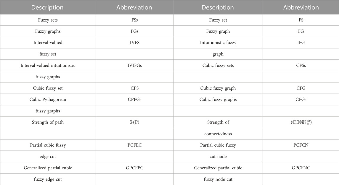
Table 1. Abbreviations.
2 Preliminaries
This section is composed of elementary ideas affiliated with CFGs.
Definition 2.1. [46]. A CFS X on a non-empty set V is described as
where [σ−(dw), σ+(dw)] is named as the IVF-membership value and
Definition 2.2. [48]. A CFG over the set V is a pair
Definition 2.3. [48]. A CFG
•
•
Definition 2.4. [48]. A CFG
∀dw−1, dw ∈ B.
Definition 2.5. [48]. A cubic fuzzy path
The strength of cubic fuzzy path
where
The strength of connectedness
where
The path
Definition 2.6. [52]. Let
1. If
2. If
3. If
Definition 2.7. [52]. A CFG
• α-saturated if at each node of σ*, there are incident n ≥ 1 α-strong edges to it
• β-saturated if at each node of σ*, there are incident n ≥ 1 β-strong edges to it
• saturated if it is α- as well as β-saturated
• unsaturated if it is neither α- nor β-saturated
Example 2.8. consider a CFG
The connectivity among the pairs (i, j), (k, l), (j, l), and (i, k) is computed as follows:
From Equation 1, if we follow Definition 2.6, it is clear that ij and kl are α-strong edges and ik and jl are β-strong edges. If we follow Definition 2.7 CFG
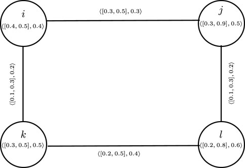
Figure 1.
3 Vertex and edge connectivity in a CFG
In this section, we present the notion of a partial cubic fuzzy cut node, cubic fuzzy vertex connectivity, partial cubic fuzzy edge cut, and cubic fuzzy edge connectivity and engage in a thorough exploration of their pertinent findings.
Definition 3.1. A collection of cubic fuzzy vertices denoted as X = v1, v2, … , vn ⊂ σ* within a cubic fuzzy graph
If Eq. (2) holds, then a set of cubic fuzzy vertices is referred to as an IVF cut node, whereas if Eq. (2) and Eq. (3) is satisfied, then it is referred to as an F cut node. If both Eq. (2) are satisfied for the same pair of vertices, then it is referred to as a strict cubic fuzzy cut node. If X contains n vertices, then X is referred to as an n-PCFCN.
Definition 3.2. Let X be a partial cubic fuzzy cut node in
where μ−(t, z), μ+(t, z) and
Definition 3.3. The cubic fuzzy vertex connectivity of
Definition 3.4. Considering
Considering
Definition 3.5. For a CF edge dw−1dw in a CFG, if one of the following holds, then dw−1, dw is called a partial cubic α-strong edge.
1.
2.
The CF α-strong is defined in [52]. However, we note that there are CFGs which contain edges which are either IVF α-strong and F β-strong or IVF β-strong and F α-strong but not CF α-strong. These types of edges seem very close to CF α-strong edges and may be more useful in different CF connectivity problems. The following example is helpful to understand this situation:
Example 3.6. consider a CFG
The connectivity for the pair i, j is computed as
It is clear that the edge ij is an IVF α-strong edge but an F β-strong edge. We can see that if we slightly increase the value of the F-membership of edge ij, then it becomes a CF α-strong edge. So, we can say that it is very close to a CF α-strong edge. This example motivates us to define the concept of partial cubic α-strong edge.
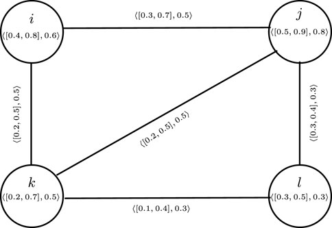
Figure 2.
Definition 3.7. For a CF edge dw−1dw in a CFG, if one of the following holds, then dw−1dw is called a partial cubic δ-weak edge.
1.
2.
Definition 3.8. A CFG
• partial α-saturated if at each node of σ*, there are incident n ≥ 1 partial α-strong edges to it
• β-saturated if at each node of σ*, there are incident n ≥ 1 β-strong edges to it
• partial saturated if it is partial α-saturated as well as β-saturated
Definition 3.9. Considering
If Eq. (4) holds, then a set of strong edges is referred to as an IVF edge cut, whereas if Eq. (5) is satisfied, then it is referred to as an F edge cut. If both Eq. (4) and Eq. (5) are satisfied for the same pair of vertices, then it is referred to as a strict cubic fuzzy edge cut. If E contains n edges, then E is referred to as an n-PCFEC.
Definition 3.10. Let E be a partial cubic fuzzy edge cut in
Definition 3.11. The cubic fuzzy edge connectivity of
Example 3.12. consider a CFG
Thus, from Table 2, the cubic fuzzy edge connectivity is
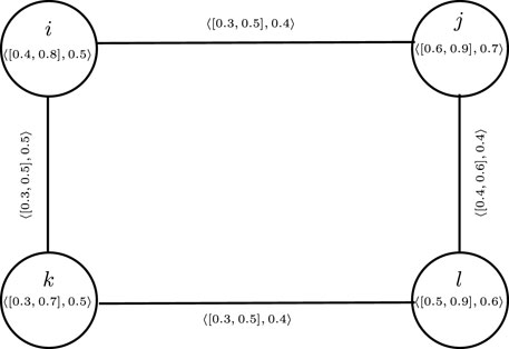
Figure 3.
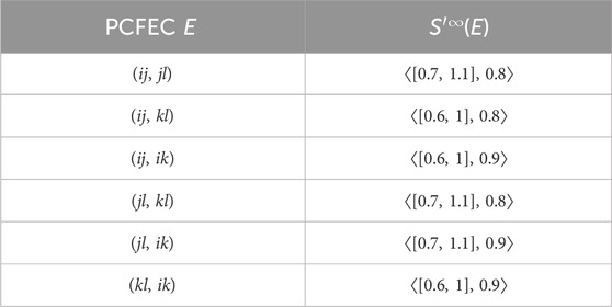
Table 2. PCFEC of
Definition 3.13. Let
or
If Eq. (6) holds, then
or
If Eq. (8) holds, then
Definition 3.14. A CFG graph
Theorem 3.15. Considering
Proof. Let S be any partial cubic fuzzy edge cut in Q. If Q−S becomes disconnected, then clearly R−S will also become disconnected. Thus, in this case, each partial cubic fuzzy edge cut of Q is also a partial cubic fuzzy edge cut of R with
If the pair a, b or any other pair satisfied Eq. (10) and Eq. (11) in R, then again
Example 3.16. consider a CFG
E = {ij} is a 1-PCFEC because for the pair kl,
From Equation 14,
From Equation 15,
From Equation 16,
Now, we consider
E = {ij} is a unique 1-PCFEC because
From Equations 17 and 18, it can be seen that Theorem 3.15 does not generally hold for every partial cubic fuzzy subgraph.
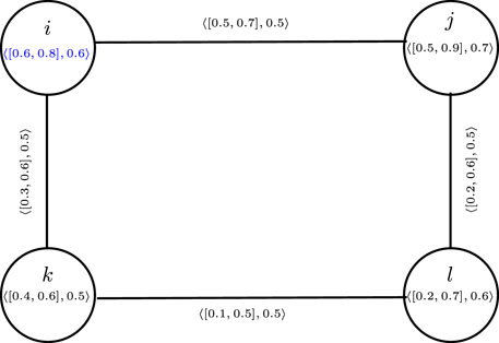
Figure 4.
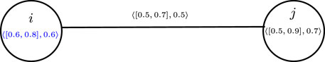
Figure 5.
Theorem 3.17. consider a cubic fuzzy cycle
where tv is the β-strong edge of
Proof. Suppose
Since
This implies that
This shows that s1s2 is either IVF α-strong or F α-strong. This, along with the fact that
Thus, removing a single edge within
Example 3.18. consider a CFG
Thus, from Table 3, we have
ij and kl are both the same weakest edge in a given graph
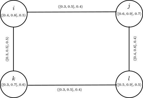
Figure 6.

Table 3. PCFEC of
Theorem 3.19. consider
where bc is the β-strong edge in
Proof. We consider
Example 3.20. consider a CFG
Thus, from Table 4, we have
ik and jl are both strong edges with the same minimum cubic membership in a given graph
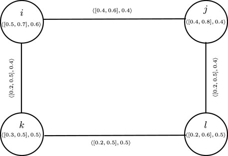
Figure 7.
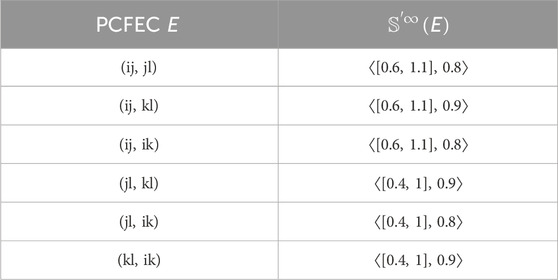
Table 4. PCFEC of
4 Generalized cubic fuzzy vertex and edge connectivity
The concepts of cubic fuzzy cut node and cubic fuzzy edge cut are generalized in this section. It is evident that not only strong edges but also non-strong edges play a significant role in maintaining the connectivity of cubic fuzzy graphs. Additionally, the requirement that both t and v should differ from the endpoints of edges in E renders a cubic fuzzy edge cut invalid, as it extends beyond the conventional set of edges. Consequently, the definitions of cubic fuzzy vertex connectivity and cubic edge connectivity have been revised, as indicated in Definition 4.1 and Definition 4.4, respectively.
Definition 4.1. Let X be a partial cubic fuzzy cut node in
where μ−(t, z), μ+(t, z) and
Definition 4.2. Let
If Eq. (21) holds, then a set of edges is referred to as an IVF edge cut, whereas if Eq. (22) is satisfied, then it is referred to as an F edge cut. If both Eq. (21) and Eq. (22) are satisfied for the same pair of vertices, then it is referred to as a strict generalized cubic fuzzy edge cut (GCFEC). If there are n edges in E, then E is called an n-GPCFEC.
Definition 4.3. Let E be a generalized partial cubic fuzzy edge cut in
Definition 4.4. The generalized cubic fuzzy edge connectivity of
Example 4.5. consider a CFG
Thus, from Table 5, the cubic fuzzy edge connectivity is given in Eq. (23)
Thus, from Table 6, the generalized cubic fuzzy edge connectivity is given in Eq. (24)
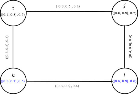
Figure 8.

Table 5. PCFEC of
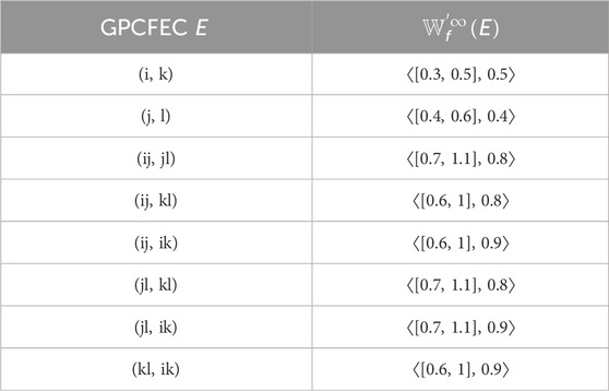
Table 6. PCFEC of
Definition 4.6. A connected CFG
1.
2.
Theorem 4.7. For a cubic fuzzy tree
where bc in Eq. (25) is a strong edge (partial α-strong or β-strong edge) in
Proof. We consider a cubic fuzzy tree
1.
2.
A non-cyclic edge in
Example 4.8. consider a cubic fuzzy tree
Thus, from Table 7, the generalized cubic fuzzy edge connectivity is given in Eq. (26)
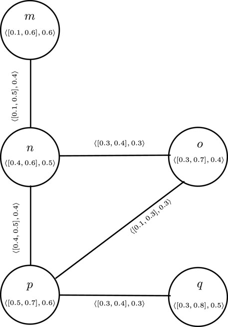
Figure 9.
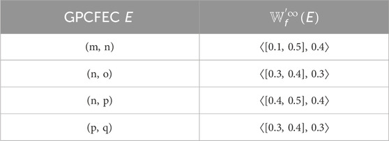
Table 7. GPCFEC of
Theorem 4.9. Let
where bc in Eq. (27) is a β-strong edge in
Proof. We consider
Theorem 4.10. Let
Proof. We consider
5 Application
Street crimes stem from various underlying causes, including socioeconomic disparities, unemployment, drug addiction, and inadequate law enforcement. These crimes, such as mugging, theft, and drug dealing, create an environment of insecurity and instability, which hampers trade relations between different regions. The occurrence of street crimes can lead to decreased investment, hinder economic growth, and result in a trade deficit between regions. Business operating in areas with high crime rates may experience decreased sales and increased costs due to theft, property damage, and heightened security measures. This can result in a decline in exports and an increase in imports, further widening the trade deficit. To improve trade flow, it is crucial to address the root causes of street crimes. This can be achieved through socioeconomic development initiatives, job creation, rehabilitation programs for offenders, and strengthening law enforcement. Furthermore, fostering community engagement, enhancing public safety measures, and promoting awareness campaigns can help to create a secure environment that encourages trade and fosters economic cooperation between regions.
5.1 Trade deficit model
This article presents the development of an application that specifically addresses the trade deficit resulting from street crimes. It explores the factors contributing to trade congestion and delves into the causes of street crimes. Furthermore, it proposes several strategies to prevent crimes and enhance trade flow. To achieve this, this study identifies regions that are particularly susceptible to trade congestion. Here, we analyze the impact of street crimes on these specific regions by using the GPCFEC. By using the CFG methodology, a trade deficit model is constructed to examine the impact of street crimes. The model assigns vertices to different regions, with lower IVF-membership values indicating past trade deficits caused by street crimes and upper IVF-membership values, suggesting the potential for future trade deficits. The F-membership value represents the current trade deficit situation resulting from street crimes. Edges in the model signify potential trade deficit zones, indicating the possibility of trade imbalances between adjacent vertices. The strength of connectedness among various regions can be used to categorize trade deficit zones. These zones can be classified as GPCFEC zones and secure zones. A secure zone indicates an area where the occurrence of a trade deficit due to street crimes is negligible; on the other hand, a GPCFEC zone represents an area where the possibility of a trade deficit resulting from street crimes exists.
A fuzzy graph is a model that visually represents the relationships among elements and their degrees of membership using vertices and edges in a two-dimensional space. However, dealing with ambiguous data using fuzzy graph theory can often be challenging. On the other hand, a CFG is an extension of the FG concept. While the memberships of vertices and edges in fuzzy graphs range from 0 to 1, a CFG holds greater significance as it assigns both lower and upper IVF-membership and F-membership values to its vertices and edges. Each membership value can be any real number within the range of [0,1], making the CFG more versatile and flexible compared to the FG. A CFG proves to be a valuable instrument for handling partial knowledge relationships among regions and effectively managing knowledge loss within a given system. In this regard, an algorithm has been devised specifically for identifying the regions impacted by trade deficits. The algorithm is provided in Table 8.

Table 8. Algorithm.
Let us consider the group of regions denoted as Y = (r1, r2, r3, r4, r5, r6), where street crimes occur. These regions can potentially be affected by trade deficits. A CFG denoted as
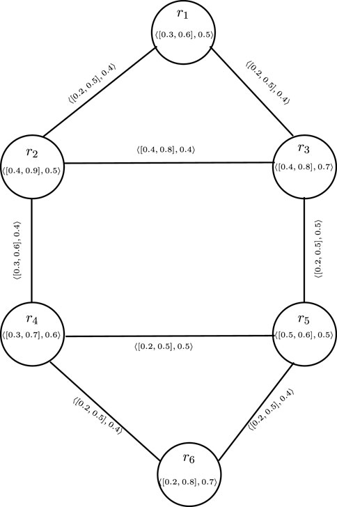
Figure 10.
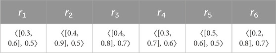
Table 9. Membership values of each vertex in CFG
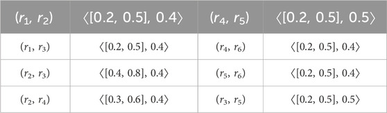
Table 10. Membership values of each edge in CFG
Table 11 provides a list of all possible paths between r2 and r4 in the CFG, along with the strengths and strength of connections among them. Specifically, the edge (r2, r4) in the CFG is represented as the GPCFEC. It is recommended to explore the nature of other edges among regions as well. Analyzing the characteristics of each edge in the CFG will further highlight the importance and effectiveness of our research. By referring to Figure 10 and using conventional computations, the connectivity between vertices in
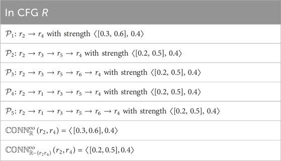
Table 11. All paths from r2 to r4 in
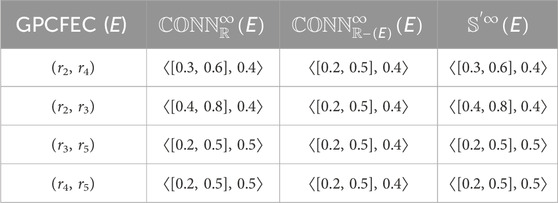
Table 12. Generalized partial cubic fuzzy edge cut of
The GPCFEC zones are determined based on specific edge conditions. In this system, the zones (r2, r4), (r2, r3), (r3, r5), and (r4, r5) satisfy the criteria for GPCFEC zones, and these zones are characterized by meeting the conditions set for the generalized partial cubic fuzzy edge cut. On the other hand, the remaining edges (r1, r2), (r1, r3), (r4, r6), and (r5, r6) do not fulfill the conditions required for GPCFEC zones and are referred to as secure zones within this specific CFG system. The categorization of regions experiencing a trade deficit into various zones can be beneficial in understanding the trade deficit situation in those regions caused by street crimes. In regions classified as the GPCFEC zone, where trade deficits are influenced by street crimes, effective planning is essential. Emergency response planning should be prioritized to ensure swift actions in addressing street crimes and their impact on trade. Additionally, enhancing public safety measures, such as increasing police presence and improving surveillance systems, can contribute to reducing criminal incidents. Promoting awareness among the public about the consequences of street crimes on trade and encouraging citizen engagement in reporting suspicious activities are important measures. In secure zones, where regions have no trade deficits, planning efforts should focus on maintaining favorable conditions and further enhancing trade flow through streamlined customs procedures, trade facilitation measures, and fostering a business-friendly environment. Overall, by planning efforts for each zone, trade regions can effectively address trade deficits caused by street crimes, promoting trade flow, economic growth, and sustainable trade surpluses.
6 Comparative analysis
The generalized partial cubic fuzzy edge cut introduces a novel extension to the existing concept of generalized fuzzy edge cut in the context of trade deficit modeling caused by street crimes. In this comparative analysis, it can be argued that the generalized partial cubic fuzzy edge cut offers certain advantages over the generalized fuzzy edge cut.
From Table 13, it can be seen that when applying the concept of generalized partial cubic fuzzy edge cut to the trade deficit model given in Figure 10, specific zones can be identified with precision. The generalized partial cubic fuzzy edge cut zones, such as (r2, r4), (r2, r3), (r3, r5), and (r4, r5), are determined based on the satisfaction of the generalized partial cubic fuzzy edge cut condition by the corresponding edges, and the remaining edges (r1, r2), (r1, r3), (r4, r6), and (r5, r6) do not satisfy this condition and are considered secure zones. On the other hand, generalized fuzzy edge cut zones such as (r3, r5) and (r4, r5) are identified through the generalized fuzzy edge cut condition, and the remaining edges (r1, r2), (r1, r3), (r2, r3), (r2, r4), (r4, r6), and (r5, r6) do not satisfy this condition and are referred to as secure zones. The generalized partial cubic fuzzy edge cut allows for a more comprehensive analysis of trade conditions. In the concept of generalized fuzzy edge cuts, only the F-membership of edges is considered. This concept assesses trade deficit conditions, taking into account either the past, present, or future. However, when discussing generalized partial cubic fuzzy edge cuts, additional factors come into play, including upper IVF-membership, lower IVF-membership, and F-membership for edges. Consequently, when we use the generalized partial cubic fuzzy edge cut concept to solve our model, we consider all these membership values concurrently, encompassing trade deficit conditions for the past, present, and future, and provide insights into trade deficit zones and secure zones. Generalized partial cubic fuzzy edge cuts surpass these limitations by encompassing all three time periods, allowing for a more comprehensive understanding of trade deficit conditions from a comparative point of view; the concept of generalized partial cubic fuzzy edge cuts offers distinct advantages over generalized fuzzy edge cuts in terms of precise zone identification and a comprehensive analysis of trade conditions in past, present, and future scenarios.
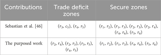
Table 13. Trade deficit zones and secure zones.
7 Conclusion
The CFG is a vital model that adeptly addresses vagueness and ambiguity in dealing with incomplete information. By incorporating lower and upper memberships, the CFG excels beyond both the fuzzy model and the interval-valued model in terms of compatibility, precision, and flexibility. This model finds extensive applications in various fields, including social circuits, machine intelligence, traffic networks, and decision-making problems. The assessment of connectivity or the strength of connectivity remains a fundamental aspect of network theory, and the CFG provides valuable insights in this regard. This paper introduces the notions of vertex and edge connectivity within cubic fuzzy graphs, accompanied by discussions on partial cubic fuzzy cut nodes and partial cubic fuzzy edge cuts. Several associated results are presented, supported by illustrative examples to facilitate comprehension. Furthermore, this research article delves into the concept of partial cubic α-strong and partial cubic δ-weak edges. An example is also presented to elucidate the rationale behind partial cubic α-strong edges. In situations where we possess information regarding the past, future, and current states of a model or problem, we can depict the past condition as a lower interval-valued fuzzy membership, the future condition as an upper interval-valued fuzzy membership, and the present condition as a fuzzy membership value. Our goal is to examine the problem by deriving lower interval-valued fuzzy connectivity, upper interval-valued fuzzy connectivity, and fuzzy connectivity. Additionally, we aspire to formulate new predictions based on this analytical approach. Moreover, it delves into the introduction of generalized vertex and edge connectivity in cubic fuzzy graphs, along with generalized partial cubic fuzzy cut nodes and generalized partial cubic fuzzy edge cuts. Relevant results pertaining to these concepts are also discussed. Furthermore, this article introduces an application that employs generalized partial cubic fuzzy edge cuts to examine the impacts of trade congestion on different regions and address vagueness and uncertainty in business-related contexts. Throughout this paper, we considered simple connected CFGs. In the realm of future research, a promising avenue for exploration lies in the amalgamation of graph theory with recent advancements in fuzzy set models. This integration could encompass the assimilation of concepts and methodologies from various fuzzy set models, including (i) (2,1)-fuzzy sets, emphasizing their properties, weighted aggregated operators, and applications in multi-criteria decision-making methods; (ii) generalized frame for orthopair fuzzy sets, investigating (m,n)-fuzzy sets and their relevance in multi-criteria decision making; and (iii) SR-fuzzy sets and their potential in weighted aggregated operators for decision making. This interdisciplinary approach holds substantial potential for advancing both graph theory and fuzzy set theory, paving the way for novel solutions to complex problems and the optimization of decision-making processes. Looking forward, this study aims to delve deeper into vertex connectivity and edge connectivity in cubic intuitionistic fuzzy graphs (CIFGs) as an expansion of the research scope.
Data availability statement
The original contributions presented in the study are included in the article/Supplementary Material; further inquiries can be directed to the corresponding author.
Author contributions
YR: formal analysis, funding acquisition, investigation, methodology, resources, and writing–review and editing. RC: conceptualization, formal analysis, funding acquisition, investigation, resources, and writing–review and editing. UA: conceptualization, formal analysis, investigation, methodology, resources, and writing–review and editing. AG: conceptualization, formal analysis, investigation, methodology, writing–original draft, and writing–review and editing.
Funding
The authors declare that financial support was received for the research, authorship, and/or publication of this article. This work was supported by the National Natural Science Foundation of China (No. 62172116).
Conflict of interest
The authors declare that the research was conducted in the absence of any commercial or financial relationships that could be construed as a potential conflict of interest.
Publisher’s note
All claims expressed in this article are solely those of the authors and do not necessarily represent those of their affiliated organizations, or those of the publisher, the editors, and the reviewers. Any product that may be evaluated in this article, or claim that may be made by its manufacturer, is not guaranteed or endorsed by the publisher.
References
3. Yeh RT, Bang SY. Fuzzy relations, fuzzy graphs and their applications to clustering analysis. Fuzzy Sets their Appl Cogn Decis Process (1975) 125–49.
4. Akram M, Sarwar M. Novel applications of m-polar fuzzy hypergraphs. J Intell Fuzzy Syst (2017) 32(3):2747–62. doi:10.3233/jifs-16859
5. Ahmad U, Batool T. Domination in rough fuzzy digraphs with application. Soft Comput (2023) 27(5):2425–42. doi:10.1007/s00500-022-07795-1
6. Ahmad U, Khan NK, Saeid AB. Fuzzy topological indices with application to cybercrime problem. Granular Comput (2023) 8:967–80. doi:10.1007/s41066-023-00365-2
7. Ahmad U, Nawaz I. Wiener index of a directed rough fuzzy graph and application to human trafficking. J Intell Fuzzy Syst (2023) 44:1479–95. doi:10.3233/jifs-221627
8. Ahmad U, Sabir M. Multicriteria decision making based on the degree and distance based indices of fuzzy graphs. Granular Comput (2022) 8:793–807. doi:10.1007/s41066-022-00354-x
9. Kou Z, Kosari S, Akhoundi M. A novel description on vague graph with application in transportation systems. J Math (2021) 2021:1–11. doi:10.1155/2021/4800499
10. Shao Z, Kosari S, Shoaib M, Rashmanlou H. Certain concepts of vague graphs with applications to medical diagnosis. Front Phys (2020) 8:357. doi:10.3389/fphy.2020.00357
11. Qiang X, Akhoundi M, Kou Z, Liu X, Kosari S. Novel concepts of domination in vague graphs with application in medicine. Math Probl Eng (2021) 2021:1–10. doi:10.1155/2021/6121454
12. Shao Z, Kosari S, Rashmanlou H, Shoaib M. New concepts in intuitionistic fuzzy graph with application in water supplier systems. Mathematics (2020) 8:1241. doi:10.3390/math8081241
13. Shi X, Kosari S, Talebi AA, Sadati SH, Rashmanlou H. Investigation of the main energies of picture fuzzy graph and its applications. Int J Comput Intelligence Syst (2022) 15(1):31. doi:10.1007/s44196-022-00086-5
14. Rao Y, Kosari S, Anitha J, Rajasingh I, Rashmanlou H. Forcing parameters in fully connected cubic networks. Mathematics (2022) 10(8):1263. doi:10.3390/math10081263
15. Akram M, Davvaz B. Strong intuitionistic fuzzy graphs. Filomat (2012) 26(1):177–96. doi:10.2298/fil1201177a
16. Harary F, Norman RZ. Graph theory as a mathematical model in social science, Ann Arbor: University of Michigan, Institute for Social Research (1953).
17. Kosari S, Rao Y, Jiang H, Liu X, Wu P, Shao Z. Vague graph Structure with Application in medical diagnosis. Symmetry (2020) 12(10):1582. doi:10.3390/sym12101582
18. Mandal S, Pal M. Connectivity index of m-polar fuzzy graph with application (2021). https://www.researchsquare.com/article/rs-737239/v11.
19. Sebastian A, Mordeson JN, Mathew S. Generalized fuzzy graph connectivity parameters with application to human trafficking. Mathematics (2020) 8(3):424. doi:10.3390/math8030424
20. Mathew S, Sunitha MS. Node connectivity and arc connectivity of a fuzzy graph. Inf Sci (2010) 180(4):519–31. doi:10.1016/j.ins.2009.10.006
21. Mathew S, Sunitha MS. Cycle connectivity in fuzzy graphs. J Intell Fuzzy Syst (2013) 24(3):549–54. doi:10.3233/ifs-2012-0573
22. Banerjee S. An optimal algorithm to find the degrees of connectedness in an undirected edge-weighted graph. Pattern Recognition Lett (1991) 12(7):421–4. doi:10.1016/0167-8655(91)90316-e
23. Ali S, Mathew S, Mordeson JN, Rashmanlou H. Vertex connectivity of fuzzy graphs with applications to human trafficking. New Math Nat Comput (2018) 14(03):457–85. doi:10.1142/s1793005718500278
24. Ahmad U, Nawaz I. Directed rough fuzzy graph with application to trade networking. Comput Appl Math (2022) 41(8):366. doi:10.1007/s40314-022-02073-0
25. Shang Y. Super connectivity of erdos-rényi graphs. Mathematics (2019) 7(3):267. doi:10.3390/math7030267
26. Su G, Wang S, Du J, Gao M, Das KC, Shang Y. Sufficient conditions for a graph to Be ℓ-connected, ℓ-deficient, ℓ-Hamiltonian and ℓ−-independent in terms of the forgotten topological index. Mathematics (2022) 10(11):1802. doi:10.3390/math10111802
27. Jun YB, Smarandache F, Kim CS. Neutrosophic cubic sets. New Math Nat Comput (2017) 13(01):41–54. doi:10.1142/s1793005717500041
28. Amer A, Naeem M, Rehman HU, Irfan M, Saleem MS, Yang H. Edge version of topological degree based indices of Boron triangular nanotubes. J Inf Optimization Sci (2020) 41(4):973–90. doi:10.1080/02522667.2020.1743505
29. Irfan M, Rehman HU, Almusawa H, Rasheed S, Baloch IA. M-polynomials and topological indices for line graphs of chain silicate network and h-naphtalenic nanotubes. J Math (2021) 2021:1–11. doi:10.1155/2021/5551825
30. Sunitha MS, Vijayakumar A. A characterization of fuzzy trees. Inf Sci (1999) 113:293–300. doi:10.1016/s0020-0255(98)10066-x
31. Mathew S, Yang HL, Mathew JK. Saturation in fuzzy graphs. New Math Nat Comput (2018) 14(01):113–28. doi:10.1142/s1793005718500084
33. Bhutani KR, Rosenfeld A. Fuzzy end nodes in fuzzy graphs. Inf Sci (2003) 152:323–6. doi:10.1016/s0020-0255(03)00078-1
34. Talebi AA, Rashmanlou H, Mehdipoor N. Isomorphism on vague graphs. Ann Fuzzy Math Inform (2013) 6(3):575–88.
35. Talebi AA, Rashmanlou H. Complement and isomorphism on bipolar fuzzy graphs. Fuzzy Inf Eng (2014) 6(4):505–22. doi:10.1016/j.fiae.2015.01.007
36. Mathew S, Sunitha MS. Types of arcs in a fuzzy graph. Inf Sci (2009) 179(11):1760–8. doi:10.1016/j.ins.2009.01.003
37. Karunambigai MG, Parvathi R, Buvaneswari R. Arcs in intuitionistic fuzzy graphs. Notes on Intuitionistic Fuzzy Sets (2011) 17(4):37–47.
38. Akram M, Siddique S, Ahmad U. Menger’s theorem for m-polar fuzzy graphs and application of m-polar fuzzy edges to road network. J Intell Fuzzy Syst (2021) 41(1):1553–74. doi:10.3233/jifs-210411
39. Naeem T, Gumaei A, Kamran Jamil M, Alsanad A, Ullah K. Connectivity indices of intuitionistic fuzzy graphs and their applications in internet routing and transport network flow. Math Probl Eng (2021) 2021:1–16. doi:10.1155/2021/4156879
40. Binu M, Mathew S, Mordeson JN. Cyclic connectivity index of fuzzy graphs. IEEE Trans Fuzzy Syst (2020) 29(6):1340–9. doi:10.1109/tfuzz.2020.2973941
41. Zadeh LA. The concept of a linguistic variable and its application to approximate reasoning-I. Inf Sci (1975) 8(3):199–249. doi:10.1016/0020-0255(75)90036-5
42. Akram M. Interval-valued fuzzy line graphs. Neural Comput Appl (2012) 21:145–50. doi:10.1007/s00521-011-0733-0
43. Talebi AA, Rashmanlou H, Sadati SH. New concepts on m-polar interval-valued intuitionistic fuzzy graph. TWMS J Appl Eng Math (2020) 10(3):806–18.
44. Talebi AA, Rashmanlou H, Sadati SH. Interval-valued intuitionistic fuzzy competition graph. J Multiple-Valued Logic Soft Comput (2020) 34:335–64.
45. Rashmanlou H, Borzooei RA. New concepts of interval-valued intuitionistic (S, T)-fuzzy graphs. J Intell Fuzzy Syst (2016) 30(4):1893–901. doi:10.3233/ifs-151900
47. Rashid S, Yaqoob N, Akram M, Gulistan M. Cubic graphs with application. Int J Anal Appl (2018) 16(5):733–50. doi:10.28924/2291-8639
48. Muhiuddin G, Takallo MM, Jun YB, Borzooei RA. Cubic graphs and their application to a traffic flow problem. Int J Comput Intelligence Syst (2020) 13(1):1265–80. doi:10.2991/ijcis.d.200730.002
49. Fang G, Ahmad U, Rasheed A, Khan A, Shafi J. Planarity in cubic intuitionistic graphs and their application to control air traffic on a runway. Front Phys (2023) 11. doi:10.3389/fphy.2023.1254647
50. Muhiuddin G, Hameed S, Maryam A, Ahmad U. Cubic Pythagorean fuzzy graphs. J Math (2022) 2022:1–25. doi:10.1155/2022/1144666
51. Muhiuddin G, Hameed S, Rasheed A, Ahmad U. Cubic planar graph and its application to road network. Math Probl Eng (2022) 2022:1–12. doi:10.1155/2022/5251627
Keywords: vertex and edge connectivity in CFGs, generalized cubic fuzzy vertex and edge connectivity, trade deficit, strong edges, cubic fuzzy graph
Citation: Rao Y, Chen R, Ahmad U and Ghafar Shah A (2024) Generalized connectivity in cubic fuzzy graphs with application in the trade deficit problem. Front. Phys. 11:1328116. doi: 10.3389/fphy.2023.1328116
Received: 26 October 2023; Accepted: 26 December 2023;
Published: 21 March 2024.
Edited by:
Song Zheng, Zhejiang University of Finance and Economics, ChinaReviewed by:
Yilun Shang, Northumbria University, United KingdomHamood Ur Rehman, University of Okara, Pakistan
Ganesh Ghorai, Vidyasagar University, India
Copyright © 2024 Rao, Chen, Ahmad and Ghafar Shah. This is an open-access article distributed under the terms of the Creative Commons Attribution License (CC BY). The use, distribution or reproduction in other forums is permitted, provided the original author(s) and the copyright owner(s) are credited and that the original publication in this journal is cited, in accordance with accepted academic practice. No use, distribution or reproduction is permitted which does not comply with these terms.
*Correspondence: Uzma Ahmad, uzma.math@pu.edu.pk