Entropy bound for time reversal markers

1 Introduction

A common way of analyzing complex systems is observation of particle trajectories, e.g., via microscopy [1–3] in biological systems [4–8] or complex fluids [9, 10]. Detecting and quantifying the deviation from equilibrium, i.e., the violation of detailed balance, based on trajectories is, however, a challenging task, especially if relevant degrees of freedom are hidden, and non-equilibrium processes are random [11–17]. Several methods for such detection have been developed.

The fluctuation dissipation theorem (FDT) connects fluctuations and response functions [18], and it is violated out of equilibrium [19–21]. How far away from equilibrium a system is, e.g., has been quantified by using the so-called effective temperatures or effective energies [22–27].

Another way of detecting broken detailed balance is via entropy production, which has been found to obey a variety of theorems including the fluctuation theorems [28–31]. A number of important relations have been found that bound entropy production, such as the thermodynamic uncertainty relation (TUR) [32–38]. The TUR bounds mean and variance of currents by entropy production or vice versa. It has been extended and refined, including path antisymmetric observables (FTUR) or to more general path weights [39–42] and has been applied to experiments and numerical data [43–46]. Little is, however, known about how bounds behave under coarse graining.

In this paper, we derive an entropy bound in terms of the mean of path-antisymmetric observables, based on an integrated fluctuation theorem. In contrast to the TUR and FTUR, it does not involve the variance of the observable. We determine the optimal observable, i.e., the observable that maximizes the bound, to be the signum of entropy production so that a relation between entropy production and its sign appears. As this relation saturates for a binary process at short times, we argue that no better relation between entropy production and its sign can exist with the same range of validity. The sign of entropy production, and hence the bound for entropy production, can be preserved under coarse graining with a simple path grouping rule. We apply these results for a discrete network on a ring. For this network, the signum of entropy production is coarse-grained under preservation to the signum of the traveled distance, demonstrating how a bound for microscopic entropy production is obtained from a macroscopic observable. Under such coarse graining, entropy production can at most reduce to the original bound.

2 Setup and fluctuation theorem

A path observable $O\left[\omega \right]$ is considered, with path ω in the phase space, with path probability p[ω], and the average is formally given by the sum over paths [47] $⟨O⟩=\int \mathcal{D}\omega O\left[\omega \right]p[\omega ]$. To construct a marker for path reversal, the sum is reordered [48]

$2⟨O⟩=\int \mathcal{D}\omega \left\{O\left[\omega \right]p\left[\omega \right]+O\left[\theta \omega \right]p\left[\theta \omega \right]\right\}.(1)$

We introduced notation for path reversal, θω, including reversal of time and of kinematic reversal of momenta [49]. Validity of Eq. 1 requires the sum of paths to include θω for any included ω. Adding a zero yields

$\begin{array}{cc}\hfill 2⟨O⟩& =\int \mathcal{D}\omega \left\{\left(O\left[\omega \right]+O\left[\theta \omega \right]\right)p\left[\theta \omega \right]\right.\hfill \\ \hfill & +\left.O\left[\omega \right]\left(p\left[\omega \right]-p\left[\theta \omega \right]\right)\right\},\hfill \end{array}(2)$

where the term $O\left[\omega \right]+O\left[\theta \omega \right]$ in the first line of Eq. 2 is the path symmetric part of O:

$O\left[\omega \right]+O\left[\theta \omega \right]\equiv 2O_{+}\left[\omega \right].(3)$

With detailed balance obeyed, i.e., p[ω] = p[θω], antisymmetric observables average to zero, and

$⟨O⟩\stackrel{\text{d.b.}}{=}⟨O_{+}⟩.(4)$

Violations of Eq. 4, thus, indicate the breakage of detailed balance [50, 51]. Although the symmetric part O₊ does not appear in the final result, Eq. 12 below, for the derivation, it is useful to start with O₊ finite.

To quantify the path reversal properties of cases that break detailed balance, we introduce the stochastic change in entropy defined as the log ratio of path probabilities (k_B = 1) [52–54].

$s=\log \frac{p\left[\omega \right]}{p\left[\theta \omega \right]}.(5)$

For simplicity, we will, in the following, refer to s as the entropy production despite some caveats regarding this term¹. The thermodynamic relevance of s is a topic of its own, which has been discussed in various works [52–54]. Substituting s into Eq. 2 yields

$2⟨O⟩=2⟨O_{+}⟩+\int \mathcal{D}\omega O\left[\omega \right]\left(1-e^{-s}\right)p\left[\omega \right].(6)$

Reordering the terms yields a fluctuation theorem including O:

$⟨O\left(1+e^{-s}\right)⟩=2⟨O_{+}⟩.(7)$

Equation 7 may be found equivalently from the so-called strong detailed fluctuation theorem [48] and has been stated in the similar form [50].

3 Entropy bound

Equation 7 can be used to find bounds for s, and we, therefore, restrict to positive observables, O[ω] ≥ 0. This allows Jensen’s inequality [55, 56] to be applied for the average $⟨O\dots ⟩/⟨O⟩$, to obtain from Eq. 7,

$\frac{2⟨O_{+}⟩-⟨O⟩}{⟨O⟩}=\frac{⟨O{e}^{-s}⟩}{⟨O⟩}\ge e^{-\frac{⟨Os⟩}{⟨O⟩}}.(8)$

As expected from Jensen’s inequality, Eq. 8 saturates for small s, as seen by expanding it in this limit,

$\frac{⟨O{e}^{-s}⟩}{⟨O⟩}=1-\frac{⟨Os⟩}{⟨O⟩}+\mathcal{O}\left(s^2\right)=e^{-\frac{⟨Os⟩}{⟨O⟩}}+\mathcal{O}\left(s^2\right).(9)$

Taking the logarithm of Eq. 8 yields a lower bound for the correlation $⟨Os⟩$:²

$\log \left(\frac{⟨O⟩}{2⟨O_{+}⟩-⟨O⟩}\right)\le \frac{⟨Os⟩}{⟨O⟩}.(10)$

Because the conjugate observable O*[ω] = O[θω] is non-negative if O is non-negative, Eq. 10 is also valid for O*. The bounds for $⟨Os⟩$ and $⟨O^{*}s⟩$ may, thus, be added to arrive at a bound for $⟨s{O}_{+}⟩$, the correlation of s, and the symmetric part O₊:

$2⟨s{O}_{+}⟩\ge \left(⟨O⟩-⟨O^{*}⟩\right)\log \left(\frac{⟨O⟩}{⟨O^{*}⟩}\right).(11)$

Notably, when adding Eq. 10 for $⟨Os⟩$ and $⟨O^{*}s⟩$, the linear term in Eq. 9 drops out so that Eq. 11 does, in general, not saturate for small s. As will be discussed below, it saturates for a binary process for short times, for any value of s.

A direct way to extract a bound for $⟨s⟩$ from Eq. 11 is by considering O₊ = 1, i.e., path-independent. In order for O to be positive, the antisymmetric part, 2O₋[ω] = O[ω] − O[θω], must be normalized to $\left|O_{-}[\omega ]\right|\le 1$. This yields the following equation:

$⟨s⟩\ge ⟨O_{-}⟩\log \left(\frac{1+⟨O_{-}⟩}{1-⟨O_{-}⟩}\right)\ge 0.(12)$

Equation 12 is a main result of this paper, a bound for entropy production $⟨s⟩$ in terms of the average of the antisymmetric observable O₋. This relation is, thus, fundamentally different from uncertainty relations, which bound entropy production in terms of mean and variance [40].

The condition of $\left|O_{-}[\omega ]\right|\le 1$ may seem to be a strong restriction of validity of Eq. 12. However, a bound between $⟨s⟩$ and $⟨O_{-}⟩$ can only be useful if O₋ is normalizable, i.e., if a maximum value of $\underset{\omega }{\max }|O_{-}|<\infty$ exists. Whenever this maximum exists, O₋ can be normalized to fulfill $\left|O_{-}[\omega ]\right|\le 1$. Eq. 12 is, thus, applicable for any normalizable antisymmetric observable. We also note that the right hand side of Eq. 12 is non-negative so that any non-zero $⟨O_{-}⟩$ yields a positive bound for $⟨s⟩$.

Equation 12 can be read in the following two ways: (i) a given $⟨s⟩$ yields a bound for how far the mean of (any) O₋ can deviate from zero. Using, e.g., a time interval from −t₀ to t₀, O₋ can be the time-moment at which a certain event occurs, which is then bound by $⟨s⟩$ via Eq. 12. This will be investigated in future works. (ii) A given non-vanishing value of $⟨O_{-}⟩$ yields a lower bound for entropy production. We will analyze this below.

The form of Eq. 12 is illustrated in Figure 1. For small $⟨O_{-}⟩$, the bound grows quadratically in $⟨O_{-}⟩$, while it diverges logarithmically for $⟨O_{-}⟩\to 1$.

FIGURE 1

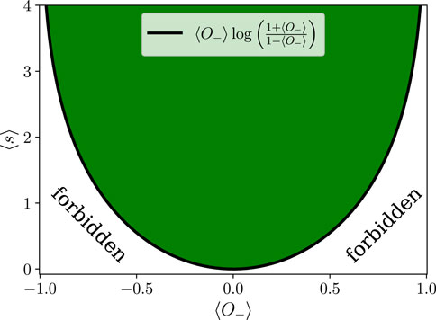
FIGURE 1. Illustration of Eq. 12 in terms of antisymmetric observable $⟨O_{-}⟩$, with the accessible area marked in green. For $⟨O_{-}⟩\to \pm 1$, the bound diverges logarithmically.

4 Optimal observable: signum of entropy

Equation 12, as mentioned, is valid for any normalizable antisymmetric observable, and, naturally, the observable that maximizes the right hand side of it yields the best estimate for $⟨s⟩$. Which observable is it? Answering this important question has been found non-trivial for entropy bounds [58, 59], while it has a clear answer for Eq. 12. To see this, rewrite³

$\begin{array}{ll}\hfill ⟨O_{-}⟩& ={\displaystyle \sum _{\omega }}{O}_{-}\left[\omega \right]p\left[\omega \right]=\frac{1}{2}{\displaystyle \sum _{\omega }}{O}_{-}\left[\omega \right]\left(p\left[\omega \right]-p\left[\theta \omega \right]\right)\hfill \\ \hfill & \le ⟨\text{sign}\left(s\right)⟩.\hfill \end{array}(13)$

In the second step, we used the anti-symmetry of O₋. The inequality in the last step of Eq. 13 follows by noting that the sum is maximized if O₋[ω] = 1 for p[ω] > p[θω] and O₋[ω] = −1 for p[ω] < p[θω]. This is the definition of O₋ = sign(s)⁴.

As the right hand side of Eq. 12 is a monotonically growing function of $|⟨O_{-}⟩|$ (compare Figure 1), O₋ = sign(s) yields the optimal bound for $⟨s⟩$ from Eq. 12. To emphasize this, we write explicitly

$\begin{array}{ll}\hfill ⟨s⟩& \ge ⟨\text{sign}(s)⟩\log \left(\frac{1+⟨\text{sign}(s)⟩}{1-⟨\text{sign}(s)⟩}\right)\hfill \\ \hfill & \ge ⟨O_{-}⟩\log \left(\frac{1+⟨O_{-}⟩}{1-⟨O_{-}⟩}\right).\hfill \end{array}(14)$

The first inequality of Eq. 14 bounds $⟨s⟩$ by $⟨\text{sign}(s)⟩$. Writing $⟨\text{sign}(s)⟩=\frac{1}{2}{\sum }_{\omega }\text{sign}(p[\omega ]-p[\theta \omega ])(p[\omega ]-p[\theta \omega ])$ shows that $⟨\text{sign}(s)⟩\ge 0$ and that $⟨\text{sign}(s)⟩=0$ only if $⟨s⟩=0$, i.e., Eq. 14 yields a finite bound for any finite $⟨s⟩$. The second inequality of Eq. 14 restates that O₋ = sign(s) yields the optimal bound so that any other O₋ lies below it.

5 Coarse graining

A bound of $⟨s⟩$ in terms of $⟨\text{sign}(s)⟩$ is fundamentally interesting, and it is also useful, as, e.g., $⟨\text{sign}(s)⟩$ has beneficial properties under coarse graining. Therefore, consider coarse-grained paths Ω with probabilities P(Ω) = ∑_ω∈Ωp(ω) and coarse-grained entropy production $S=\log \frac{P[\mathrm{\Omega }]}{P[\theta \mathrm{\Omega }]}$. Naturally, O₋ = sign(S) fulfills Eq. 13 so that for any grouping of paths,

$0\le ⟨\text{sign}(S)⟩\le ⟨\text{sign}(s)⟩.(15)$

Coarse graining, thus, leads, in general, to a decrease in $⟨\text{sign}(s)⟩$, reminiscent of the finding that $⟨s⟩$ also decreases under coarse graining [60]. Notably, grouping paths according to the sign of s, i.e., with sign(s[ω]) = sign(S[Ω_o]) conserves $⟨\text{sign}(s)⟩$.

$⟨\text{sign}(s)⟩=\frac{1}{2}{\displaystyle \sum _{{\mathrm{\Omega }}_o}}\text{sign}\left(P\left[{\mathrm{\Omega }}_o\right]-P\left[\theta {\mathrm{\Omega }}_o\right]\right)\times$

$\times {\displaystyle \sum _{\omega \in {\mathrm{\Omega }}_o}}\left(p\left[\omega \right]-p\left[\theta \omega \right]\right)$

$=⟨\text{sign}(S_o)⟩.(16)$

Under this “optimal” (index o) coarse graining, the bound provided by sign(s) is invariant so that the macroscopic $⟨\text{sign}(S_o)⟩$ yields the same bound as the microscopic $⟨\text{sign}(s)⟩$. Furthermore, as the bound must hold for s and S_o alike, coarse-grained entropy production S_o never falls below the original, microscopic bound. This algorithm, thus, provides a controlled coarse graining of entropy production, which is especially useful if the bound from sign(s) is close to s.

6 Example: network on a ring

To display this in an example, consider a network on a ring, where every state is connected to two neighbors (see inset sketch of Figure 2). In every discrete time step, a particle jumps to the left (right) with probability p (q). For q ≠ p, the system violates detailed balance and shows a directed flow. After N steps, the probability of finding a specific path with n_L steps to the left is given by the binomial distribution $p[\omega ]=\frac{1}{L}{p}^{n_L}{q}^{N-n_L}$, with L the number of states in the network. With it, entropy production after N steps is given by the following equation:

$⟨s⟩=N\left(p-q\right)\log \left(\frac{p}{q}\right).(17)$

FIGURE 2

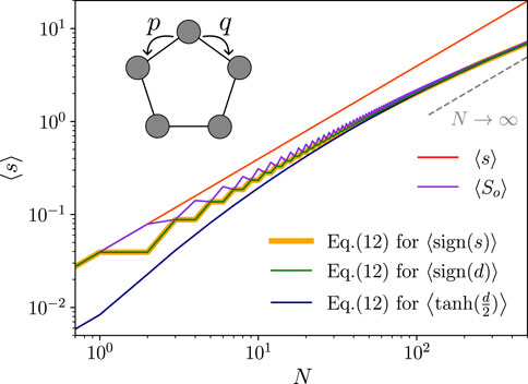
FIGURE 2. Network on a ring model: entropy production $⟨s⟩$ as a function of N, Eq. 17, for p =0.57, versus the bound obtained from Eq. 12 for various observables as sign(s), sign(d) and $\tanh (\frac{d}{2})$ using numerical simulations. The gray dotted line is the asymptotic limit of large N. The graph also shows optimally coarse-grained entropy $⟨S_o⟩$.

Optimal coarse graining can be performed here in a straightforward manner: because s = d log(p/q), the sign of entropy production equals the sign of d = n_L − n_R (for p > q), with n_R being the number of steps to the right, i.e., sign(d[ω]) = sign(s[ω]). This system, thus, allows coarse graining toward the measurement of the net displacement d, under preservation of the bound. We may expect that d is easier to measure than s.

Having established that Eq. 12 is maximal for O₋ = sign(d[ω]), we can test the quality of the estimate for $⟨s⟩$ provided by it. For N = 1, $⟨\text{sign}(d)⟩=p-q$ and

$⟨s⟩\stackrel{N=1}{=}⟨\text{sign}\left(d\right)⟩\log \left(\frac{1+⟨\text{sign}\left(d\right)⟩}{1-⟨\text{sign}\left(d\right)⟩}\right).(18)$

For N = 1, the bound of Eq. 12, thus, meets entropy production exactly, for any p and q, i.e., arbitrarily far from equilibrium. This is the abovementioned case of the binary process, where a particle either jumps right or left.

Figure 2 shows $⟨s⟩$ and the bound of Eq. 12 as a function of N. For N > 1, the bound grows sublinear in N for an intermediate range and, thus, falls below the value of s. For N ≫ 1, it approaches a linear asymptote, which can be found via a large deviation principle. We find for $p>\frac{1}{2}$ and N → ∞ [61],

$⟨\text{sign}(s)⟩=⟨\text{sign}\left(d\right)⟩\sim 1-\frac{2}{1-\frac{q}{p}}\frac{{\left(\frac{1}{4pq}\right)}^{-\frac{N}{2}}}{\sqrt{\frac{\pi }{2}N}},(19)$

i.e., $⟨\text{sign}(d)⟩$ approaches unity exponentially fast with N. Because of this, the bound for s of Eq. 12 grows linear in N, and substituting (19) into Eq. 12 yields $\frac{1}{2}\log \left(\frac{1}{4pq}\right)N$, shown as a gray line in the graph. The ratio between this large N asymptote and $⟨s⟩$ of Eq. 17 varies between $\frac{1}{2}$ for p → 1 and $\frac{1}{4}$ for $p\to \frac{1}{2}$.

Coarse graining groups paths according to their displacement, i.e., Ω for d > 0 and θΩ for d < 0. This way, the coarse-grained entropy $⟨S_o⟩$ can be determined, which is also shown in Figure 2. The curve demonstrates that it, as expected, stays above the bound. As only two coarse grained paths with finite S_o exist, it is obtained from.

$⟨S_o⟩=\log \left(\frac{P\left[{\mathrm{\Omega }}_o\right]}{P\left[\theta {\mathrm{\Omega }}_o\right]}\right)P\left[{\mathrm{\Omega }}_o\right],$

$+\log \left(\frac{P\left[\theta {\mathrm{\Omega }}_o\right]}{P\left[{\mathrm{\Omega }}_o\right]}\right)P\left[\theta {\mathrm{\Omega }}_o\right].(20)$

$\stackrel{N\mathrm{o}\mathrm{d}\mathrm{d}}{=}⟨\text{sign}\left(d\right)⟩\log \left(\frac{1+⟨\text{sign}\left(d\right)⟩}{1-⟨\text{sign}\left(d\right)⟩}\right).(21)$

Notably, the bound shown in Eq. 12 is saturated with respect to S_o for odd N, as indicated. For N even, paths with zero entropy production exist, and the second equality shown in Eq. 21 is not valid, and Eq. 12 lies below $⟨S_o⟩$. For large N, these differences vanish so that the bound of Eq. 12 and $⟨S_o⟩$ share the same asymptote. In this system, entropy production may, thus, be coarse-grained by a maximal loss of a factor between 2 and 4, depending on p, using the optimal algorithm.

According to Eq. 13, any other normalizable antisymmetric observable should yield a lower bound, which we exemplify by using O₋ = tanh(d/2). Indeed, it lies lower but approaches the optimal bound for large N because then, a typical trajectory shows d ≫ 1 so that tanh(d/2) becomes equivalent to sign(d).

Although optimal coarse graining is possible in an exact manner in this model, we expect an approximate preservation of sign(s) to be possible in more complicated systems, which will be investigated in future works.

Can we compare to other relations such as TUR? The original TUR is not applicable to time-discrete dynamics, as used in this example. We, thus, compare to the so-called FTUR [40], as shown in Figure 3. Not knowing the optimal observable for FTUR, we use sign(s) and s, analytically computing the required variances for these two. Interestingly, for each of the three curves shown in the figure, there exists a regime of N, where it provides the highest estimate. It is also remarkable that FTUR used with sign(s) can provide a better estimate compared to using s. This shows the advantage of Eq. 17, for which the optimal observable is known, leading to the coarse-graining scheme. It also shows that the comparison between these relations is rich and non-trivial and needs to be studied in future works.

FIGURE 3

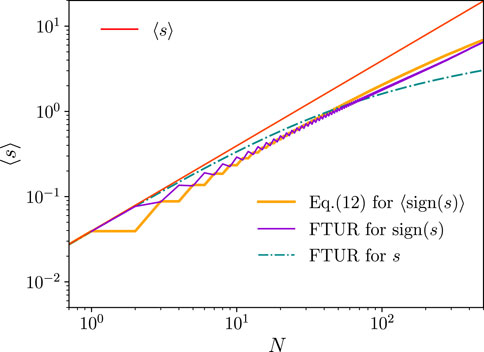
FIGURE 3. Network on a ring model, with identical parameters as shown in Figure 2, here focusing on the comparison to FTUR. FTUR is used with two different observables as indicated, sign(s) or s. For large N, Eq. 12 and FTUR for the sign(s) scale linearly in N, while FTUR for s scales with log(N).

7 Discussion

Entropy production is bound by the mean of normalizable antisymmetric observables. The optimal observable is identified to be the signum of entropy production so that we determine a bound between entropy production and its sign, sign(s). The latter may often be estimated from simple observables, like here, the displacement on a ring. The network example shows that measuring sign(s) (did the particle move left or right?) is expected to require a lower experimental resolution compared to measuring s (where did the particle move when?). One can also estimate ⟨sign(s)⟩ by the use of Eq. (13), i.e., by testing various observables O₋ and finding the maximum deviation from zero. For the investigated network, $⟨\text{sign}(s)⟩$ approaches unity exponentially fast with the number of steps so that the bound grows with the expected linear dependence. Grouping paths according to sign(s) yields a coarse-graining algorithm that preserves sign(s) and the bound. The presented analysis is not restricted to specific dynamics. Due to this, it is, additionally to the here-discussed discrete system, also valid for fluids and biological systems [27]. Future work may investigate applications to Langevin systems as well, like active Brownian particles, or quantum mechanics [62–65].

Data availability statement

The raw data supporting the conclusion of this article will be made available by the authors, without undue reservation.

Author contributions

GK: writing–original draft. TM: writing–review and editing. TB: writing–review and editing. MK: writing–original draft.

Funding

The author(s) declare that no financial support was received for the research, authorship, and/or publication of this article.

Acknowledgments

The authors thank É. Fodor for a critical reading of the paper and Peter Sollich and Cai Dieball for insightful discussions. The authors acknowledge support by the Open Access Publication Funds of the Göttingen University.

Conflict of interest

The authors declare that the research was conducted in the absence of any commercial or financial relationships that could be construed as a potential conflict of interest.

Publisher’s note

All claims expressed in this article are solely those of the authors and do not necessarily represent those of their affiliated organizations, or those of the publisher, the editors, and the reviewers. Any product that may be evaluated in this article, or claim that may be made by its manufacturer, is not guaranteed or endorsed by the publisher.

Footnotes

¹The entropy defined in Eq. 5 corresponds to the total change in entropy in overdamped stationary systems. In underdamped or non-stationary systems, the boundary terms differ [54].

²A similar relation was derived in [57], however, with the left hand side always negative.

³Eq. 13 holds also for −O₋ and thus for $|⟨O_{-}⟩|$.

⁴The terms with p[ω] = p[θω] cancel in the sum in Eq. 13 due to O₋[ω] = −O₋[θω], and O₋[ω] can be chosen arbitrarily in these cases.

References

1. Squires TM, Mason TG. Fluid mechanics of microrheology. Annu Rev Fluid Mech (2010) 42:413–38. doi:10.1146/annurev-fluid-121108-145608

CrossRef Full Text | Google Scholar

2. Zia RN. Active and passive microrheology: theory and simulation. Annu Rev Fluid Mech (2018) 50:371–405. doi:10.1146/annurev-fluid-122316-044514

CrossRef Full Text | Google Scholar

3. Bustamante CJ, Chemla YR, Liu S, Wang MD. Optical tweezers in single-molecule biophysics. Nat Rev Methods Primers (2021) 1:25. doi:10.1038/s43586-021-00021-6

PubMed Abstract | CrossRef Full Text | Google Scholar

4. Fang X, Wang J. Nonequilibrium thermodynamics in cell biology: extending equilibrium formalism to cover living systems. Annu Rev Biophys (2020) 49:227–46. doi:10.1146/annurev-biophys-121219-081656

PubMed Abstract | CrossRef Full Text | Google Scholar

5. Andrieux D, Gaspard P. Fluctuation theorems and the nonequilibrium thermodynamics of molecular motors. Phys Rev E (2006) 74:011906. doi:10.1103/PhysRevE.74.011906

PubMed Abstract | CrossRef Full Text | Google Scholar

6. Ahmed WW, Fodor É, Betz T. Active cell mechanics: measurement and theory. Biochim Biophys Acta (Bba) - Mol Cel Res (2015) 1853:3083–94. doi:10.1016/j.bbamcr.2015.05.022

PubMed Abstract | CrossRef Full Text | Google Scholar

7. Gladrow J, Broedersz CP, Schmidt CF. Nonequilibrium dynamics of probe filaments in actin-myosin networks. Phys Rev E (2017) 96:022408. doi:10.1103/PhysRevE.96.022408

PubMed Abstract | CrossRef Full Text | Google Scholar

8. Hurst S, Vos BE, Brandt M, Betz T. Intracellular softening and increased viscoelastic fluidity during division. Nat Phys (2021) 17:1270–6. doi:10.1038/s41567-021-01368-z

CrossRef Full Text | Google Scholar

9. Mason TG, Weitz DA. Optical measurements of frequency-dependent linear viscoelastic moduli of complex fluids. Phys Rev Lett (1995) 74:1250–3. doi:10.1103/PhysRevLett.74.1250

PubMed Abstract | CrossRef Full Text | Google Scholar

10. Ginot F, Caspers J, Krüger M, Bechinger C. Barrier crossing in a viscoelastic bath. Phys Rev Lett (2022) 128:028001. doi:10.1103/PhysRevLett.128.028001

PubMed Abstract | CrossRef Full Text | Google Scholar

11. Roldán É, Parrondo JMR. Estimating dissipation from single stationary trajectories. Phys Rev Lett (2010) 105:150607. doi:10.1103/PhysRevLett.105.150607

PubMed Abstract | CrossRef Full Text | Google Scholar

12. Mehl J, Lander B, Bechinger C, Blickle V, Seifert U. Role of hidden slow degrees of freedom in the fluctuation theorem. Phys Rev Lett (2012) 108:220601. doi:10.1103/PhysRevLett.108.220601

PubMed Abstract | CrossRef Full Text | Google Scholar

13. Basu U, Helden L, Krüger M. Extrapolation to nonequilibrium from coarse-grained response theory. Phys Rev Lett (2018) 120:180604. doi:10.1103/PhysRevLett.120.180604

PubMed Abstract | CrossRef Full Text | Google Scholar

14. Kahlen M, Ehrich J. Hidden slow degrees of freedom and fluctuation theorems: an analytically solvable model. J Stat Mech Theor Exp (2018) 2018:063204. doi:10.1088/1742-5468/aac2fd

CrossRef Full Text | Google Scholar

15. Martínez IA, Bisker G, Horowitz JM, Parrondo JMR. Inferring broken detailed balance in the absence of observable currents. Nat Commun (2019) 10:3542. doi:10.1038/s41467-019-11051-w

PubMed Abstract | CrossRef Full Text | Google Scholar

16. Dieball C, Godec A. Coarse graining empirical densities and currents in continuous-space steady states. Phys Rev Res (2022) 4:033243. doi:10.1103/PhysRevResearch.4.033243

CrossRef Full Text | Google Scholar

17. van der Meer J, Ertel B, Seifert U. Thermodynamic inference in partially accessible markov networks: a unifying perspective from transition-based waiting time distributions. Phys Rev X (2022) 12:031025. doi:10.1103/PhysRevX.12.031025

CrossRef Full Text | Google Scholar

18. Kubo R. The fluctuation-dissipation theorem. Rep Prog Phys (1966) 29:255–84. doi:10.1088/0034-4885/29/1/306

CrossRef Full Text | Google Scholar

19. Agarwal GS. Fluctuation-dissipation theorems for systems in non-thermal equilibrium and applications. Z für Physik A Hadrons nuclei (1972) 252:25–38. doi:10.1007/BF01391621

CrossRef Full Text | Google Scholar

20. Speck T, Seifert U. Restoring a fluctuation-dissipation theorem in a nonequilibrium steady state. Europhysics Lett (Epl) (2006) 74:391–6. doi:10.1209/epl/i2005-10549-4

CrossRef Full Text | Google Scholar

21. Baiesi M, Maes C, Wynants B. Fluctuations and response of nonequilibrium states. Phys Rev Lett (2009) 103:010602. doi:10.1103/PhysRevLett.103.010602

PubMed Abstract | CrossRef Full Text | Google Scholar

22. Martin P, Hudspeth AJ, Jülicher F. Comparison of a hair bundle’s spontaneous oscillations with its response to mechanical stimulation reveals the underlying active process. Proc Natl Acad Sci (2001) 98:14380–5. doi:10.1073/pnas.251530598

PubMed Abstract | CrossRef Full Text | Google Scholar

23. Harada T, Si S. Equality connecting energy dissipation with a violation of the fluctuation-response relation. Phys Rev Lett (2005) 95:130602. doi:10.1103/PhysRevLett.95.130602

PubMed Abstract | CrossRef Full Text | Google Scholar

24. Toyabe S, Okamoto T, Watanabe-Nakayama T, Taketani H, Kudo S, Muneyuki E. Nonequilibrium energetics of a single F 1 -ATPase molecule. Phys Rev Lett (2010) 104:198103. doi:10.1103/PhysRevLett.104.198103

PubMed Abstract | CrossRef Full Text | Google Scholar

25. Krüger M, Fuchs M. Fluctuation dissipation relations in stationary states of interacting brownian particles under shear. Phys Rev Lett (2009) 102:135701. doi:10.1103/PhysRevLett.102.135701

PubMed Abstract | CrossRef Full Text | Google Scholar

26. Ahmed WW, Fodor É, Almonacid M, Bussonnier M, Verlhac MH, Gov N, et al. Active mechanics reveal molecular-scale force kinetics in living oocytes. Biophysical J (2018) 114:1667–79. doi:10.1016/j.bpj.2018.02.009

CrossRef Full Text | Google Scholar

27. Muenker TM, Knotz G, Krüger M, Betz T. Onsager regression characterizes living systems in passive measurements (2022). bioRxiv. doi:10.1101/2022.05.15.491928

CrossRef Full Text | Google Scholar

28. Jarzynski C. Nonequilibrium equality for free energy differences. Phys Rev Lett (1997) 78:2690–3. doi:10.1103/PhysRevLett.78.2690

CrossRef Full Text | Google Scholar

29. Crooks GE. Entropy production fluctuation theorem and the nonequilibrium work relation for free energy differences. Phys Rev E (1999) 60:2721–6. doi:10.1103/PhysRevE.60.2721

PubMed Abstract | CrossRef Full Text | Google Scholar

30. Speck T, Seifert U. The jarzynski relation, fluctuation theorems, and stochastic thermodynamics for non-markovian processes. J Stat Mech Theor Exp (2007) 2007:L09002. doi:10.1088/1742-5468/2007/09/L09002

CrossRef Full Text | Google Scholar

31. Seifert U. Stochastic thermodynamics, fluctuation theorems and molecular machines. Rep Prog Phys (2012) 75:126001. doi:10.1088/0034-4885/75/12/126001

PubMed Abstract | CrossRef Full Text | Google Scholar

32. Barato AC, Seifert U. Thermodynamic uncertainty relation for biomolecular processes. Phys Rev Lett (2015) 114:158101. doi:10.1103/PhysRevLett.114.158101

PubMed Abstract | CrossRef Full Text | Google Scholar

33. Horowitz JM, Gingrich TR. Thermodynamic uncertainty relations constrain non-equilibrium fluctuations. Nat Phys (2020) 16:15–20. doi:10.1038/s41567-019-0702-6

CrossRef Full Text | Google Scholar

34. Van Vu T, Vo VT, Hasegawa Y. Entropy production estimation with optimal current. Phys Rev E (2020) 101:042138. doi:10.1103/PhysRevE.101.042138

PubMed Abstract | CrossRef Full Text | Google Scholar

35. Dechant A, Si S. Improving thermodynamic bounds using correlations. Phys Rev X (2021) 11:041061. doi:10.1103/PhysRevX.11.041061

CrossRef Full Text | Google Scholar

36. Pietzonka P. Classical pendulum clocks break the thermodynamic uncertainty relation. Phys Rev Lett (2022) 128:130606. doi:10.1103/PhysRevLett.128.130606

PubMed Abstract | CrossRef Full Text | Google Scholar

37. Cao Z, Su J, Jiang H, Hou Z. Effective entropy production and thermodynamic uncertainty relation of active Brownian particles. Phys Fluids (2022) 34:053310. doi:10.1063/5.0094211

CrossRef Full Text | Google Scholar

38. Koyuk T, Seifert U. Thermodynamic uncertainty relation in interacting many-body systems. Phys Rev Lett (2022) 129:210603. doi:10.1103/PhysRevLett.129.210603

PubMed Abstract | CrossRef Full Text | Google Scholar

39. Dechant A, Si S. Current fluctuations and transport efficiency for general Langevin systems. J Stat Mech Theor Exp (2018) 2018:063209. doi:10.1088/1742-5468/aac91a

CrossRef Full Text | Google Scholar

40. Hasegawa Y, Van Vu T. Fluctuation theorem uncertainty relation. Phys Rev Lett (2019) 123:110602. doi:10.1103/PhysRevLett.123.110602

PubMed Abstract | CrossRef Full Text | Google Scholar

41. Dechant A, Si S. Fluctuation–response inequality out of equilibrium. Proc Natl Acad Sci (2020) 117:6430–6. doi:10.1073/pnas.1918386117

PubMed Abstract | CrossRef Full Text | Google Scholar

42. Ziyin L, Ueda M. Universal thermodynamic uncertainty relation in nonequilibrium dynamics. Phys Rev Res (2023) 5:013039. doi:10.1103/PhysRevResearch.5.013039

CrossRef Full Text | Google Scholar

43. Li J, Horowitz JM, Gingrich TR, Fakhri N. Quantifying dissipation using fluctuating currents. Nat Commun (2019) 10:1666. doi:10.1038/s41467-019-09631-x

PubMed Abstract | CrossRef Full Text | Google Scholar

44. Manikandan SK, Ghosh S, Kundu A, Das B, Agrawal V, Mitra D, et al. Quantitative analysis of non-equilibrium systems from short-time experimental data. Commun Phys (2021) 4:258. doi:10.1038/s42005-021-00766-2

CrossRef Full Text | Google Scholar

45. Otsubo S, Manikandan SK, Sagawa T, Krishnamurthy S. Estimating time-dependent entropy production from non-equilibrium trajectories. Commun Phys (2022) 5:11–0. doi:10.1038/s42005-021-00787-x

CrossRef Full Text | Google Scholar

46. Roldán Barral J, Martin P, Parrondo JMR, Jülicher F, Jülicher F. Quantifying entropy production in active fluctuations of the hair-cell bundle from time irreversibility and uncertainty relations. New J Phys (2021) 23:083013. doi:10.1088/1367-2630/ac0f18

CrossRef Full Text | Google Scholar

47. Altland A, Simons BD. Condensed matter field theory. 2 edn. Cambridge: Cambridge University Press (2010). doi:10.1017/CBO9780511789984

CrossRef Full Text | Google Scholar

48. García-García R, Domínguez D, Lecomte V, Kolton AB. Unifying approach for fluctuation theorems from joint probability distributions. Phys Rev E (2010) 82:030104. doi:10.1103/PhysRevE.82.030104

CrossRef Full Text | Google Scholar

49. Spinney RE, Ford IJ. Entropy production in full phase space for continuous stochastic dynamics. Phys Rev E (2012) 85:051113. doi:10.1103/PhysRevE.85.051113

PubMed Abstract | CrossRef Full Text | Google Scholar

50. Harris RJ, Schütz GM. Fluctuation theorems for stochastic dynamics. J Stat Mech Theor Exp (2007) 2007:P07020. doi:10.1088/1742-5468/2007/07/P07020

CrossRef Full Text | Google Scholar

51. Zia RKP, Schmittmann B. Probability currents as principal characteristics in the statistical mechanics of non-equilibrium steady states. J Stat Mech Theor Exp (2007) 2007:P07012. doi:10.1088/1742-5468/2007/07/P07012

CrossRef Full Text | Google Scholar

52. Maes C, Netočný K. Time-reversal and entropy. J Stat Phys (2003) 110:269–310. doi:10.1023/A:1021026930129

CrossRef Full Text | Google Scholar

53. Seifert U. Entropy production along a stochastic trajectory and an integral fluctuation theorem. Phys Rev Lett (2005) 95:040602. doi:10.1103/PhysRevLett.95.040602

PubMed Abstract | CrossRef Full Text | Google Scholar

54. Fischer LP, Chun HM, Seifert U. Free diffusion bounds the precision of currents in underdamped dynamics. Phys Rev E (2020) 102:012120. doi:10.1103/PhysRevE.102.012120

PubMed Abstract | CrossRef Full Text | Google Scholar

55. Jensen JLWV. Sur les fonctions convexes et les inégalités entre les valeurs moyennes. Acta Mathematica (1906) 30:175–93. doi:10.1007/BF02418571

CrossRef Full Text | Google Scholar

56. Durrett R. Cambridge series in statistical and probabilistic mathematics. 5 edn. Cambridge, England: Cambridge University Press (2019).Probability:Theory and examples

Google Scholar

57. Merhav N, Kafri Y. Statistical properties of entropy production derived from fluctuation theorems. J Stat Mech Theor Exp (2010) 2010:P12022. doi:10.1088/1742-5468/2010/12/P12022

CrossRef Full Text | Google Scholar

58. Shiraishi N. Optimal thermodynamic uncertainty relation in markov jump processes. J Stat Phys (2021) 185:19. doi:10.1007/s10955-021-02829-8

CrossRef Full Text | Google Scholar

59. Dieball C, Godec A. Direct route to thermodynamic uncertainty relations and their saturation. Phys Rev Lett (2023) 130:087101. doi:10.1103/PhysRevLett.130.087101

PubMed Abstract | CrossRef Full Text | Google Scholar

60. Seifert U. From stochastic thermodynamics to thermodynamic inference. Annu Rev Condensed Matter Phys (2019) 10:171–92. doi:10.1146/annurev-conmatphys-031218-013554

CrossRef Full Text | Google Scholar

61. Arratia R, Gordon L. Tutorial on large deviations for the binomial distribution. Bull Math Biol (1989) 51:125–31. doi:10.1007/BF02458840

PubMed Abstract | CrossRef Full Text | Google Scholar

62. Bechinger C, Di Leonardo R, Löwen H, Reichhardt C, Volpe G, Volpe G. Active particles in complex and crowded environments. Rev Mod Phys (2016) 88:045006. doi:10.1103/RevModPhys.88.045006

CrossRef Full Text | Google Scholar

63. Esposito M, Harbola U, Mukamel S. Nonequilibrium fluctuations, fluctuation theorems, and counting statistics in quantum systems. Rev Mod Phys (2009) 81:1665–702. doi:10.1103/RevModPhys.81.1665

CrossRef Full Text | Google Scholar

64. Landi GT, Paternostro M. Irreversible entropy production: from classical to quantum. Rev Mod Phys (2021) 93:035008. doi:10.1103/RevModPhys.93.035008

CrossRef Full Text | Google Scholar

65. Aron C, Biroli G, Cugliandolo L. (Non) equilibrium dynamics: a (broken) symmetry of the Keldysh generating functional. SciPost Phys (2018) 4:008. doi:10.21468/SciPostPhys.4.1.008

CrossRef Full Text | Google Scholar