Evaluation of TIEGCM based on GOCE neutral density

1 Introduction

Although the Earth’s thermosphere is relatively sparse, it occupies a large volume. The thermosphere is not only an important field of Solar-Terrestrial space but also the main working area of low Earth orbit satellites. The thermosphere has complex thermodynamic, photochemical, and kinetic processes, which are closely related to the development of industry especially spaceflight. Therefore, the study and modeling of the thermosphere have important significance for scientific research and aerospace activities.

Since the middle of the 20th century, with the launch of a large number of satellites and the development of high-altitude detection technology, numerous observations of the thermosphere have been obtained. These datasets have greatly promoted the understanding of the upper atmosphere. GOCE satellite, developed and launched by the European Space Agency, is one of the most advanced detection satellites [1]. Thanks to the gravity gradiometers carried on board the satellites, GOCE datasets are commonly used to determine the geoid and the Earth’s gravity field [2–4]. Meanwhile, they also provide a great opportunity for studying thermospheric neutral wind and mass density. [5] presented an iterative algorithm for determining density and crosswind from multiaxis accelerometer measurements on GOCE. [6,7] used GOCE neutral densities and cross-track winds near 260 km to demonstrate vertical coupling in this height regime due to the ultra-fast Kelvin Wave (UFKW) and the eastward propagating diurnal tide with zonal wave number 3 (DE3). [8] studied the seasonal variation of the thermospheric mass density of GOCE at dawn/dusk. Similarly, [9] investigated the annual and semi-annual variations of the dawn/dusk thermospheric mass density over a certain altitude range based on the neutral density of the GOCE satellite. [10] used GOCE trans-orbital wind measurements to explore the intra-annual oscillations (IAOs) of the upper thermospheric winds between 70° S and 70° N.

With the accumulation of observations, modeling work has also prominently developed in the past few decades. The thermospheric models can be generally grouped in two categories, empirical models and physical models. Empirical models capture the statistically average behavior of the atmosphere in a parameterized mathematical formulation and usually output temperature and density are as a function of position, solar activity, geomagnetic activity and season [11]. Widely used thermospheric empirical models include the Jacchia [12–15], the Drag Temperature Model (DTM) [16–21], the Mass Spectrometer and Incoherent Scatter (MSIS) [22–25], Jacchia-Bowman (JB) [26,27], the Marshall Engineering Thermosphere Model (MET) [28–31], etc.

Physical models are also known as the first-principles models which describe the complex coupling process in the mesosphere, thermosphere, ionosphere, and magnetosphere system through a series of energy equations, dynamic equations, continuity equations, and chemical equations [32]. With the improvement of computer performance, thermospheric physical models have been developed significantly, such as the Thermosphere-Ionosphere-Electrodynamics General Circulation Model (TIEGCM), the Coupled Thermosphere Ionosphere Plasmasphere Electrodynamics Model (CTIPe) [33–35], and the Whole Atmosphere Community Climate Model with thermosphere and ionosphere extension (WACCM-X) [36,37]. Among the physical models mentioned above, the National Center for Atmospheric Research (NCAR)’s TIEGCM is one of the most advanced models which has been widely used in ionosphere and thermosphere research and achieved fruitful results [38–48,48–50,52–54].

Since GOCE satellites provide high-precision atmospheric density data in the lower thermosphere, they are also used in model accuracy assessment exercises. [55] presented the first analytical assessment of a thermosphere model against the High Accuracy Satellite Drag Model (HASDM). Their results showed that the density of HASDM and GOCE scaled by a constant factor of 1.29 are identical on time scales of 1 day or more. [56] compared the JB2006 model with the J70, MET, NRLMSIS and DTM models in terms of altitude, latitude, local time, day of year, solar radiation and geomagnetic conditions. Their studies showed that the average values of model accuracies are similar in the altitude region below 600 km. By using neutral thermospheric mass density data obtained from CHAMP (Challenging Minisatellite Payload), GRACE (Gravity Recovery and Climate Experiment) and GOCE, [19] compared the DTM2013, DTM2009 and JB2008 models. Their results displayed that the performance of these average climate models weakens as the weather contribution becomes larger. Moreover, [57] compared the NRLMISE-00, DTM2009, and DTM2013 models to provide a comprehensive assessment of the semi-empirical models. The evaluation uses three time scales, which are year, month, and day, with model performance decreasing sequentially on shorter time scales. To specify and predict fluctuations in thermospheric density during geomagnetic storms, [21] used CHAMP, GRACE, and GOCE measurements to assess the modeling capabilities of five thermospheric models for different geomagnetic storm periods. Their results concluded that DTM2013 and TIEGCM obtained the best results throughout all storm period. In addition to being directly used for evaluating models, GOCE data can also be used for assimilating models. [58] used the DTM2013, which assimilates 4 years of GOCE data, to conduct a comprehensive comparison with the remaining 11 representative models. Their results show that the scale heights of different empirical models show good agreement during periods of high solar activity.

The above studies have used GOCE neutral density to evaluate thermospheric empirical modes. This study aims to compare the GOCE neutral density with the TIEGCM density to evaluate TIEGCM. Section 2 describes the satellite density data, space weather indices used in this paper, and TIEGCM. The main results of the time-scale and space-scale analyses are given in Section 3. The conclusions are in Section 4.

2 Model and data

2.1 GOCE density data

The GOCE satellite is considered to be the first European satellite to provide a model of the global gravity field using high-precision and high-spatial-resolution technology [41]. GOCE orbited as close to Earth as possible to maximize its sensitivity to variations in Earth’s gravity field with unprecedented accuracy and spatial resolution. The satellite adopts a near-circular polar orbit with an orbital height of 295 km and an orbital inclination of 96.5° [59,60].

The high-precision thermospheric mass densities used in this paper benefit from these two important payloads on the GOCE satellite. One of the components is a combined GPS/GLONASS receiver with a 1-s sampling rate to measure high orbital pseudo-range and phase function GOCE satellites for tracking and positioning. The high-precision satellite orbit determination helps in the calibration of accelerometers and the calculation of atmospheric density [5]. The other core instrument is the triaxial electrostatic gravity gradiometer, which is used to obtain high-precision satellite gravity gradient values [17,61,62]. The non-conservative forces acting on the gravity gradiometer can be compensated by a drag-free control system (undamped ion micro-thruster).

The data used in this study extrapolate the density between the scientific mission thruster data from 1 November 2009 to 20 October 2013. The spatial resolution of the GOCE neutral density in orbit is about 80 km and the temporal resolution is 10 s. The GOCE density has a worst accuracy of a few percent, and it is better than one percent after 2010 [63]. A detailed description of the specific derivation process and validation of the GOCE dataset can be found in the final report on the ESA project website [64].

2.2 Solar and geomagnetic indices

The solar radio flux at 10.7 cm wavelength is an important parameter to characterize the level of solar activity, which is called the solar F10.7 index in “solar flux units” (SFU) [65]. Because of the strong correlation between F10.7 and solar EUV radiation, F10.7 is often used as a proxy for solar UV/EUV (SAT et al., 2023 [66]).

The geomagnetic indices used in this work are Kp and Ap. Kp, also known as the global 3-h magnetic index, is an index used by individual geomagnetic stations to describe the strength of geomagnetic disturbances every 3 h [67,68]. The Ap index is a global index of the intensity of full-day geomagnetic disturbances, known as the planetary equivalent daily amplitude (PEDA) [69,70].

Figure 1 illustrates F10.7, Ap and Kp between 1 November 2009 and 20 October 2013. As Figure 1 shows, the F10.7 occurred below 90 SFU before 2011, which indicates that the sun was at a low activity condition. The F10.7 increased prominently after 2011 and varied between 100 SFU and 180 SFU, suggesting that the sun was under high activity condition. The value of Ap was larger in 2012–2013 compared to the other 3 years, reaching a maximum of 87 in 2012. There were also several significant fluctuations from 2009 to 2011 and the trend was more gentle than that of 2012–2013, reaching a maximum of 55 in 2009. As can be seen from the figure, the Kp shows a similar trend to Ap. Moreover, Kp showed significant larger values from 2010 to 2013, with the maximum of 8 in 2012. This phenomenon suggests that geomagnetic activity was very active during this period. Summing up, majority of the GOCE density are observed under high solar activity condition, when the heating in the thermosphere by solar radiation and energetic particles remains in high level.

FIGURE 1

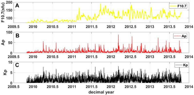
FIGURE 1. (A) F10.7 (yellow), (B) Ap (red), and (C) Kp (black) indices during 1 November 2009 and 20 October 2013.

2.3 TIEGCM

The TIEGCM developed by the NCAR’s High-Altitude Observatory (HAO), is a first-principle, time-dependent, three-dimensional model. The model uses finite difference techniques to solve the thermodynamic, and continuity equations for the middle and upper atmosphere, and takes into account the effects of particle settling in the polar regions, high-latitude electric fields, and tides from the lower atmosphere [48,71–77].

As Solomon and Qian [78] stated, the TIEGCM uses F10.7 to characterize XUV/EUV/FUV solar fluxes and thus replace solar input. By inputting indices such as F10.7 and Kp, the temperature, density, wind field, and other distributions of the global middle and upper atmosphere and its components with altitude and latitude can be calculated range extending from ∼97 km to 600 km [79]. TIEGCM has been developed to version 2.0, with a resolution of 2.5° in latitude and longitude, a vertical resolution of 1/4 scale height, and a time step of 30 s. In this work, the geomagnetic forcing to the TIEGCM model is represented by high-latitude precipitation and convection pattern of the Heelis model [80]. Besides, The TIEGCM-simulated results are interpolated to the location of GOCE observations.

3 Results

In this study, the performance of the model is evaluated by calculating the mean, standard deviation (STD) (Eq. 3) and the root mean square (RMS) (Eq. 4) of the relative deviations (Eqs 1, 2) which is calculated by the observations from the satellite and simulations from the model. The formulas for calculating the indicators used in the assessment are as follows:

$\mathit{O}-\mathit{C}={\mathit{\rho }}_{\mathit{G}\mathit{O}\mathit{C}\mathit{E}}-{\mathit{\rho }}_{\mathit{T}\mathit{I}\mathit{E}\mathit{G}\mathit{C}\mathit{M}}(1)$

$\frac{\mathit{O}-\mathit{C}}{\mathit{O}}=\frac{\left|{\mathit{\rho }}_{\mathit{G}\mathit{O}\mathit{C}\mathit{E}}-{\mathit{\rho }}_{\mathit{T}\mathit{I}\mathit{E}\mathit{G}\mathit{C}\mathit{M}}\right|}{{\mathit{\rho }}_{\mathit{G}\mathit{O}\mathit{C}\mathit{E}}}=\frac{\left|∆\mathit{\rho }\right|}{{\mathit{\rho }}_{\mathit{c}}}(2)$

$\mathit{S}\mathit{T}\mathit{D}=\left(\frac{\mathbf{1}}{\mathit{n}-\mathbf{1}}{\left.\sum _{\mathit{i}=\mathbf{1}}^{\mathit{n}}{\left(\left({\mathit{x}}_{\mathit{i}}-\overline{\mathit{x}}\right.\right)}^{\mathbf{2}}\right)}^{\frac{\mathbf{1}}{\mathbf{2}}}\right)(3)$

$\mathit{R}\mathit{M}\mathit{S}=\sqrt{\frac{\mathbf{1}}{\mathit{N}}\sum _{\mathit{i}=\mathbf{1}}^{\mathit{N}}{\left|{\mathit{x}}_{\mathit{i}}\right|}^{\mathbf{2}}}(4)$

The assessment of the model in this work will be carried out in terms of time scale analysis and spatial scale analysis. Section 3.1 presents the time-scale analysis, where the model will be evaluated in terms of yearly, monthly, and daily scales. The spatial scale analysis is presented in Section 3.2, where the model is evaluated in terms of altitude, latitude, and local time.

3.1 Performance on time scales

Figure 2 shows the time series of a) thermospheric density obtained from GOCE and TIEGCM, b) deviation between GOCE and TIEGCM, and c) relative deviation between GOCE and TIEGCM for the entire GOCE mission period from November 2009 to October 2013.

FIGURE 2

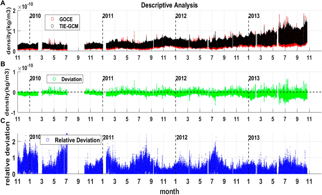
FIGURE 2. (A) GOCE density (red) and TIEGCM density (black), (B) deviation (green), (C) relative deviation (blue), during 2009–2013.

As Figure 2A shows, the observations and simulations have similar tends, i.e., the density increase with year. Combined with the results in Figure 1, this increase of density in thermosphere is mainly caused by the heating by solar radiation and energetic particles. It also should be noted that the thermospheric mass density derived from TIEGCM is slightly larger than the density derived from GOCE in general.

From Figure 2B, we can see that the deviation values are more distributed in the region of less than 0. In July 2013 and June 2011, there are a primary and a secondary peak values of the deviation, indicating that TIEGCM is underestimated by about 6.6 $\times \mathbf{10}$⁻¹¹ kg/m³ and 5.5 $\times \mathbf{10}$⁻¹¹ kg/m³, respectively. In July 2012, the deviation has a negative maximum about −6.3 $\times \mathbf{10}$⁻¹¹ kg/m³, indicating that TIEGCM overestimates the density significantly. From Figure 3, it can be seen that the observed density is larger than the simulated density around March-April and September-November each year, and the GOCE-derived density is less than the TIEGCM-simulated density around December-January and June each year. This phenomenon indicates that there is a semi-annual variation in the bias, which is most significant in 2012. In general, the fluctuation in 2009–2011 is not as prominent as that in 2012–2013, which may be related to the heating of the thermosphere by solar radiation and energetic particles.

FIGURE 3

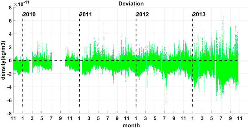
FIGURE 3. Deviation (green) during 2009–2013.

As Figure 2C shows, the relative deviation is generally larger in low solar activity years and smaller in high solar activity years, which is the opposite of the change of deviation in Figure 2B. The reason for this phenomenon is that the thermospheric density is larger in the year of high solar activity, resulting in a smaller relative deviation. In addition, we can also see the seasonal variation of relative deviations, that is, larger in winter and summer and smaller in spring and autumn. The semi-annual mentioned here are further described in long and monthly time scales.

To illustrate the distribution of the relative deviation data, Figure 4 shows the probability density function of the relative deviation with the fitted Gaussian distribution in the year of a) 2009, b) 2010, c) 2011, d) 2012, and e) 2013, respectively. The general equation for Gaussian fitting (Eq. 5) is as follows:

$\mathit{f}\left(\mathit{x}\right)={\mathit{a}}_{\mathbf{1}}*{\mathit{e}}^{{-\left(\frac{\mathit{x}-{\mathit{b}}_{\mathbf{1}}}{{\mathit{c}}_{\mathbf{1}}}\right)}^{\mathbf{2}}})+{\mathit{a}}_{\mathbf{2}}*{\mathit{e}}^{{-\left(\frac{\mathit{x}-{\mathit{b}}_{\mathbf{2}}}{{\mathit{c}}_{\mathbf{2}}}\right)}^{\mathbf{2}}})+\cdots +{\mathit{a}}_{\mathit{n}}*{\mathit{e}}^{{-\left(\frac{\mathit{x}-{\mathit{b}}_{\mathit{n}}}{{\mathit{c}}_{\mathit{n}}}\right)}^{\mathbf{2}}})(5)$

FIGURE 4

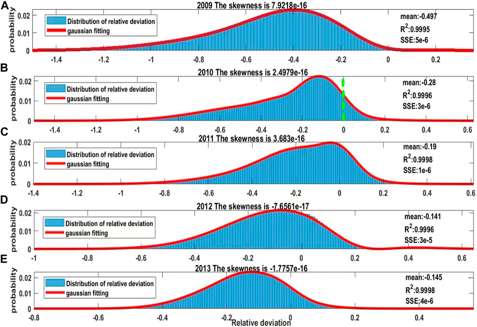
FIGURE 4. Distribution (blue) and fitted Gaussian distribution (red) of relative deviation in the year of (A) 2009, (B) 2010, (C) 2011, (D) 2012, (E) 2013.

In Figure 4A, the mean relative deviation is −0.497 which is the worst in the 5 years. While the sum of squared errors (SSE) is $\mathbf{5}\times \mathbf{10}$⁻⁶ and the R-square of the fit is 0.9995, both of which indicate that the relative deviation almost follows a Gaussian distribution. Moreover, the skewness coefficient is very small which shows the curve approximately exhibits a bell shaped symmetrical distribution. Correspondingly, in Figure 4E the relative deviation mean is less in 2013, of which the relative deviation mean is −0.145. Moreover, The SSE is $\mathbf{4}\times \mathbf{10}$⁻⁶ and the R-square of the fit is 0.9995. Overall, the Gaussian fitting effect is the best in 2013. The relevant data for other years are shown in Figures 4B–D, and they generally follow a Gaussian distribution.

Summing up, it can be seen that the relative deviation in 2009 is the largest among the 5 years. Although the skewness of the distribution of the relative deviation is closest to 0 in the 5 years, there is still a small degree of left bias (Figures 4D, E) and right bias (Figures 4A–C). In general, the data distribution is relative symmetric. From 2011 to 2012, the probability density of relative deviation near 0 is large, indicating that the sum of the data that model simulations are close to the satellite observations is large. Furthermore, the fitted R-square statistics in the 5 years are all greater than 0.99, which indicates the fitted Gaussian distribution has a good agreement.

3.1.1 Long time scales

The performance of the model on a long time scale is shown in Figure 5 and Table 1. In Table 1, it should be noted that the mean of the relative deviation for the 5 years is not equal to the mean of each year due to the different number of observations in each year. As can be seen in Figure 5 and Table 1, maximum and minimum of the mean relative deviation’s is 0.4979 in 2009 and 0.1608 in 2013, respectively. Moreover, the 5-year average is 0.2238. It also shows a decreasing trend in 5 years, and the most obvious decreasing trend occurs from 2009 to 2010. One of the possible reason of this phenomenon is relevant to the solar activities. The relative deviation is smaller because the thermospheric density is usually larger in high solar activity years. Therefore, the relative deviation is larger in 2009 when the thermospheric density is smaller. Another possible reason of the relative deviation becoming larger in 2009 is that the data for 2009 are mainly concentrated at the end of the year, which have been described in Figure 2C. Moreover, the STD of the relative deviation is the largest in 2009 and the least in 2013, which is 0.2591 and 0.1163, respectively. The 5-year average is 0.2004 which is closest to the value in 2011. Similarly, the RMS decreases monotonically from 2009 to 2013, with its maximum and minimum is 0.5613 in 2009 and 0.1984 in 2013, respectively. The average RMS of the relative deviation is 0.3004. Generally, the change trend of three indicators is quite similar in general, and the decreasing of the RMS is more prominent.

FIGURE 5

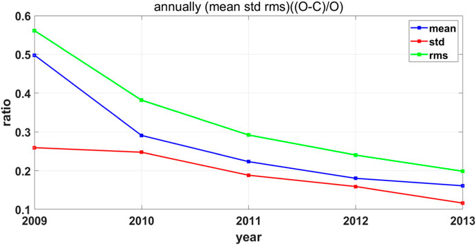
FIGURE 5. Annually means (blue), STD (red), and RMS (green) values of relative deviations of GOCE satellite and TIEGCM thermospheric density simulations from 2009 to 2013.

TABLE 1

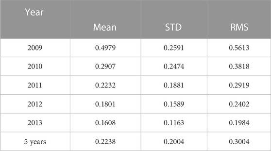
TABLE 1. Means, STD and RMS values of relative deviations of GOCE satellite and TIEGCM thermospheric density simulations from 2009 to 2013.

Consistent with Figures 1C, 5 also reflects the impact of solar activity on the density of the thermosphere atmosphere and the relative deviation of the model. In low solar activity years, the thermospheric density is small and the relative deviation is large, while in high solar activity years, the thermospheric density is large and the relative deviation is actually small.

3.1.2 Month time scales

The performance of the model on the month time scale will be described here. Figure 6 shows the mean and STD of relative deviation, and correlation between GOCE-derived and TIEGCM-simulated density. As can be seen from the figure, the monthly mean reaches a maximum of 0.63 in July 2010 and a minimum in April 2011 at 0.0825. The monthly mean exhibits larger values around December and July, and smaller values around March and September, showing a semi-annual variation. This phenomenon shows the relative deviation has primary and secondary peaks around the winter solstice and summer solstice, and minimal values around the vernal equinox and the autumnal equinox. This seasonal variation is agreeing with the results which has been shown in Figure 2C, but it is more clear here. The STD averaged on month scale shows the similar fluctuation trend as the monthly mean but its fluctuation is less significant than the mean. The peak of the STD is 0.3659 in July 2010, while the trough is 0.0651 in April 2011.The fluctuation range of the monthly mean STD is larger in the years of low solar activity in 2009–2010 than in the years of high solar activity in 2011–2013. In addition, although the correlation between GOCE observations and TIEGCM simulations fluctuates during the selected period, it has remained almost above 0.9 on average. It is worth noting that the minimum correlation coefficient of each year always appears between November and February. Among them, the minimum correlation coefficient of all years is around 0.76 in February 2013.

FIGURE 6

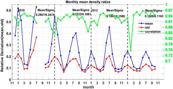
FIGURE 6. Monthly mean (blue), STD (red) of the relative deviation and correlation (green) of the GOCE satellite and TIEGCM thermospheric density simulations from 2009 to 2013.

3.1.3 Daily time scales

The performance of the model on a daily time scale is shown in Figures 7–9 and Tables 2, 3. Figure 7 shows the daily mean and STD of the relative deviations and the correlation coefficients between the daily GOCE-derived and TIEGCM-simulated density. It shows that the maximum mean of relative deviation (peak) on the daily time scale is 0.84 in 2009, while the minimum mean of it is 0.046 in 2013. Moreover, the relative deviation averaged on the daily time scales shows a similar trend of variation with the monthly mean. Furthermore, the daily STD of the relative deviation has a largest value of 0.37 in May 2010. However, the relative deviation tended to be stable, with the daily STD within 0.2. The minimum of the STD is 0.034 in 2013.The daily mean and daily STD of the relative deviation almost match those of the monthly scales in terms of the fluctuation trend, but the range of the daily mean is larger than the monthly mean. Furthermore, the minimum correlation coefficient is 0.0664 in 2011, and the maximum is 0.9869 in 2013. In general, most of the correlation coefficients are larger than 0.8, which indicating there is a high correlation between the observations and simulations on daily time scale.

FIGURE 7

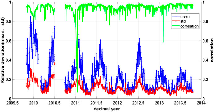
FIGURE 7. Daily mean (blue), STD (red) of the relative deviation and correlation (green) of the GOCE satellite and TIEGCM thermospheric density simulations from 2009 to 2013.

TABLE 2

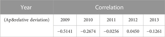
TABLE 2. Correlation between Ap and relative deviations from 2009–2013.

TABLE 3

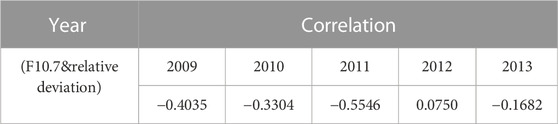
TABLE 3. Correlation between F10.7 and relative deviations from 2009–2013.

It is noticeable that [81] found that the percent difference is negatively correlated with space weather conditions. In this section, we also investigated the relationship between the relative deviation and Ap and F10.7, respectively. Figure 8 shows a time-series comparison plot of the daily mean of the relative deviation and the Ap. Meanwhile, Table 3 shows the value of the correlation coefficient between the daily relative deviation and the Ap for each year. It can be seen from Figure 8 and Table 3, the relative deviation is larger in the year with the smaller Ap index, but smaller in the year with larger Ap index. The absolute value of the correlation coefficient reaches a maximum of 0.51 in 2009 and a minimum of 0.0450 in 2012. Generally, the relative deviation and Ap show negative correlation except 2012.

FIGURE 8

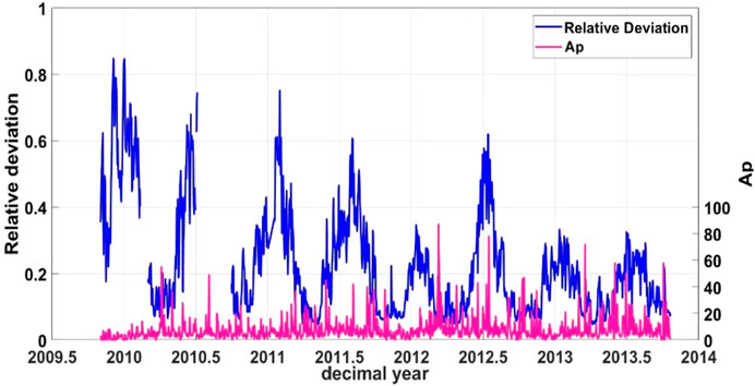
FIGURE 8. Daily average of relative deviations (blue) and Ap (pink) from 2009 to 2013.

Figure 9 shows the analysis of the daily mean relative deviation against the F10.7 for each year from 2009 to 2013. In general, the relative deviation is larger in the year with smaller F10.7 index, while the relative deviation is smaller in the year with larger F10.7 index. That is, F10.7 and relative deviation are negatively correlated overall. During high solar activity (larger F10.7), the mean of the TMD (Thermosphere Model Density) ratio is closer to 1 than during low solar activity (smaller F10.7). The TMD ratio can be converted into a relative deviation according to Eq. 2, which implies that the mean of the relative deviation is closer to 0 during high solar activity than during low solar activity. That is, the higher the level of solar activity, the smaller the relative deviation between GOCE-derived and TIEGCM-simulated density. Combined with the correlation analysis in Table 3, it can be seen that the correlation between mean relative deviation and F10.7 is strongest in 2011 with a correlation coefficient value of −0.55, followed by 2009 and 2010 with a correlation coefficient value of −0.40 and −0.33, respectively. In 2012, it shows a weak positive correlation between the F10.7 and daily average relative deviation. Therefore, except 2012, the relative deviation and F10.7 show a negative correlation. This is consistent with the conclusion reached by [58], which is concluded from empirical thermospheric models.

FIGURE 9

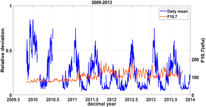
FIGURE 9. Comparative analysis of the daily average of relative deviation (blue) and F10.7 (orange) from 2009 to 2013.

To sum up, comparing Figure 6 with Table 1 and Figure 5, the relative deviation increases from 0.49 or less of the annual mean to 0.63 or less, i.e., the range of fluctuation of the relative deviation is becoming larger significantly when the model is evaluated on a shorter time scale (month). Similarly, the annually mean STD of the relative deviation increases from 0.25 or less to 0.39 or less. In other words, the range of fluctuation of the STD also becomes larger, suggesting that the model perform worse on the monthly time scale than on the longer time scale. Moreover, the relative deviation increases from 0.63 or less of the monthly mean to 0.84 or less, which also shows that the model performs better on the longer time scale.

3.2 Performance on spatial scales

3.2.1 Altitude

Figure 10 displays the relative deviation curves with altitude for each year except 2009. The altitude in each year is divided into six equal segments within its range of variation.

FIGURE 10

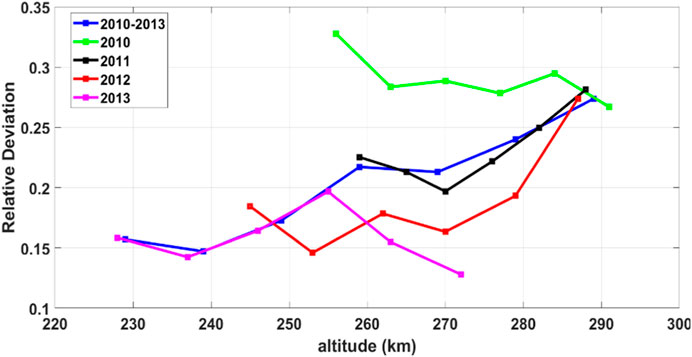
FIGURE 10. The curve of relative deviation with altitude for each selected year except 2009.

As would be expected from the data in Figure 10, the relative deviation in 2010 is systematically larger than those for the rest of the years at all altitudes. It shows that the overall trend of the relative deviation decreases with altitude in 2010. The relative deviation in 2011 is a turning point at 270 km. The relative deviation decreases with altitude that below 270 km and increases with altitude that above 270 km. Overall, the relative deviation shows an increasing trend with altitude in 2011. In 2012, the mean value of the relative deviation shows an increasing trend with altitude in the orbit altitude range, and the relative deviation increases most significantly from 279 to 287 km, which is about 0.08. The relative deviation also being a turning point at 270 km, which is the similar as that in 2011. In 2013 the relative deviation shows a definite increase with altitude that below 256 km and then decrease with altitude. The relative deviation appears a minimum at about 270 km. In addition to the treatments carried out for each year, the relative deviation with altitude is analyzed for the 4 years. The average curve of relative deviation averaged over the 4-year period has the similar trend as the 2013 curve below 240.7 km. After that the relative deviation increases with altitude. The overall trend of the 4-year relative deviation is increasing with altitude.

In order to present the true variation of relative deviation with altitude more intuitively, we averaged all altitudes by the resolution of 1 km. The result is displayed in Figure 11. It can be seen that below 290 km, the relative deviation showed a slow increasing trend. Within the range of 290–295 km, there is a significant increase in relative deviation. One of the reasons is that thermospheric density decays with altitude increase. Therefore, generally speaking, the smaller relative deviations appear at lower altitude, while the larger relative deviations occur at higher altitude. This is make an agreement with the conclusion in Figure 9, which shows that the performance of the TIEGCM may degrade as the altitude increase.

FIGURE 11

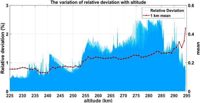
FIGURE 11. Curves of relative deviation relative to altitude change from 2009–2013 (blue) and the average of relative deviation at each altitude (black).

3.2.2 Latitude

Figure 12 shows the latitudinal structure of the models evaluated by computing relative deviation in 10° -latitude bands. In Figure 12, the relative deviation exhibits a structure of peak and trough with the variation of latitude in 2010. The peak appears at 30° N with a value of 0.32, while the trough occurs at 40° S with a value of 0.36. Furthermore, we note that the relative deviation at high latitudes is slightly larger in the Southern Hemisphere than that in the Northern Hemisphere. The relative deviation of other years has maintained a similar trend as 2010, but generally it has shown a significant decrease with year. Moreover, in other years, the maximum of relative deviation occurs in the high-latitude regions in the Southern Hemisphere, which makes the relative deviation at mid-latitude in the Northern Hemisphere become a secondary peak. That is, there is a clear hemispheric asymmetry in the latitudinal variation of relative deviations, with greater relative deviation occurs in the Southern Hemisphere except 2010.

FIGURE 12

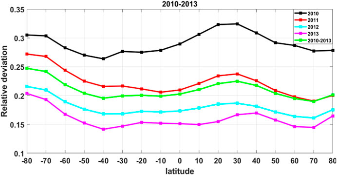
FIGURE 12. Relative deviation of GOCE and TIEGCM thermospheric density with 10° latitude bands mean for each year excep 2009.

3.2.3 Local time

In this section, we will discuss the variation of relative deviation with local time. We convert longitude into local time through the conversion Eq. 6. Due to the high inclination angle of GOCE, local time coverage is limited. In order to prevent interference from the data which is accepted from both high latitude and Cross-time zone, we exclude data with latitudes higher than 70° during our analysis.

$\mathit{L}\mathit{T}=\mathit{U}\mathit{T}+\mathit{L}\mathit{O}\mathit{N}/\mathbf{15}(6)$

Figure 13 shows the relative deviation with local time from 2010 to 2013. The relative deviation varies relative similar with local time from 2010 to 2013. The relative deviation decreases from the day side (from 5:30 LT to 7:30 LT) in 2010, reaching a minimum value of 0.287 at 7:30 LT. From 17:30 LT to 19:30 LT, the relative deviation has a significant decrease. Similar to the relative deviation of 2010, the relative deviation of 2011–2013 show the maximum deviation in local early morning and then the relative deviation rapidly decreases after that. However, the relative deviation has changed at dusk (from 17:30 LT to 20:30 LT). The relative deviation in 2011 and 2012 both show a sudden increase then decreases with local time, while the curve of 2013 is more stable from 18:30 LT to 20:30 LT. It can be seen that the relative deviation is usually larger in the dawn at about 5:30 LT, and decreases sharply to a minimum around 8:30 LT.

FIGURE 13

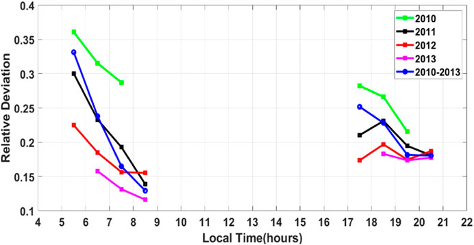
FIGURE 13. Variation of relative deviation with local time from 2010–2013.

4 Conclusion

In this paper, the density derived from the GOCE between November 2009 and October 2013 are used to validate the performance of the TIEGCM. We assess the model accuracy via both the time and spatial scales. The conclusions are as follows:

For the time scale, when assessed on the long time scale, the mean relative deviations for 2010–2013 are all within 0.30 and the STD are all within 0.25, while it had a mean relative deviation of 0.49 in 2009. In contrast, when evaluated on a monthly time scale, the mean relative deviation is below 0.1 in the April and reaches 0.63 in the July, the model bias covers a larger range, and the mean relative deviation changes from 0.49 to 0.63, an increase of 0.14. When evaluated on the daily time scale, the model bias coverage becomes larger, with the mean relative deviation changing to 0.84, a 0.21 increase from year to day. Also in the time scale, we analyzed the relationship between the daily average of relative deviation and the daily average of space weather conditions. Both Ap and F10.7 shows a negative correlation with the relative deviation, where the correlation coefficient between the relative deviation and F10.7 in 2011 is up to −0.56, i.e., The relative deviation of TIEGCM and GOCE is negatively correlated with F10.7 and Ap. The TIEGCM performs better on long-time scales than on short-time scales, which is agree with the conclusion reached by the empirical models.

For spatial scales, when assessed at altitude scales, the relative deviation regarding altitude is increased throughout the 2010–2013 years, and the relative deviation is larger at higher altitudes versus at lower altitudes. When evaluated on a latitudinal scale, by calculating the average of relative deviations in the 10°-latitude bands, it can be concluded that, there is a clear hemispheric asymmetry in the variation of relative deviations about latitude, with greater variation in the Southern Hemisphere. There is a clear hemispheric asymmetry in the latitudinal variation of relative deviations, with greater relative deviation occurs in the Southern Hemisphere except 2010. When evaluated at the local time scale, the relative deviations also show the similar structure with local time over the 4 years–they all show the relative deviation changes more dramatically in local morning than at dusk.

In summary, the high accuracy of the GOCE satellite atmospheric density data provides a good opportunity to evaluate the performance of TIEGCM at middle thermosphere. The differences between observations and simulations indicate some shortcomings of the model and thus will benefit from future model improvement.

Data availability statement

The F10.7 and Kp indices are provided by the OMNI database (https://cdaweb.gsfc.nasa.gov/). The Ap indices are provided by the website: (https://wdc.kugi.kyoto-u.ac.jp/wdc/Sec3.html). GOCE neutral density data can be obtained from the website: https://www.scidb.cn/anonymous/ZkluaVEz. The simulation data presented in this study are available on request from the corresponding author. The data are not publicly available due to privacy.

Author contributions

ZL: Conceptualization, Data curation, Formal Analysis, Funding acquisition, Investigation, Methodology, Project administration, Resources, Supervision, Writing–review and editing. JS: Conceptualization, Data curation, Formal Analysis, Investigation, Methodology, Software, Validation, Visualization, Writing–original draft, Writing–review and editing. YW: Software, Writing–review and editing. JL: Funding acquisition, Project administration, Writing–review and editing. HZ: Supervision, Writing–review and editing. CG: Writing–review and editing. XX: Funding acquisition, Project administration, Writing–review and editing.

Funding

The author(s) declare that financial support was received for the research, authorship, and/or publication of this article. This research was funded by the National Natural Science Foundation of China (grant numbers 42074183 and 42004132), and the Open Project Program of State Key Laboratory of Lunar and Planetary Sciences (Macau University of Science and Technology) (Macau FDCT grant no. SKL-LPS(MUST)-2021-2023).

Conflict of interest

The authors declare that the research was conducted in the absence of any commercial or financial relationships that could be construed as a potential conflict of interest.

Publisher’s note

All claims expressed in this article are solely those of the authors and do not necessarily represent those of their affiliated organizations, or those of the publisher, the editors and the reviewers. Any product that may be evaluated in this article, or claim that may be made by its manufacturer, is not guaranteed or endorsed by the publisher.

References

1. Visser P. GOCE gradiometer: estimation of biases and scale factors of all six individual accelerometers by precise orbit determination. J Geodesy (2009) 83(1):69–85. doi:10.1007/s00190-008-0235-8

CrossRef Full Text | Google Scholar

2. Natsiopoulos DA, Mamagiannou EG, Pitenis EA, Vergos GS, Tziavos IN. GOCE downward continuation to the Earth’s surface and improvements to local geoid modeling by FFT and LSC. Remote Sensing (2023) 15(4):991. doi:10.3390/rs15040991

CrossRef Full Text | Google Scholar

3. Brockmann JM, Schubert T, Schuh WD. An improved model of the Earth’s static gravity field solely derived from reprocessed GOCE data. Surv Geophys (2021) 42:277–316. doi:10.1007/s10712-020-09626-0

CrossRef Full Text | Google Scholar

4. Daniel A, Thomas G, Lucas S, Sterken V, Jäggi A. Reprocessed precise science orbits and gravity field recovery for the entire GOCE mission. J Geodesy (2023) 97(7):67. doi:10.1007/s00190-023-01752-y

CrossRef Full Text | Google Scholar

5. Doornbos E, Van Den Ijssel J, Luhr H, Forster M, Koppenwallner G. Neutral density and crosswind determination from arbitrarily oriented multiaxis accelerometers on satellites. J Spacecraft Rockets (2010) 47(4):580–9. doi:10.2514/1.48114

CrossRef Full Text | Google Scholar

6. Gasperini F, Forbes JM, Doornbos EN, Bruinsma SL. Wave coupling between the lower and middle thermosphere as viewed from TIMED and GOCE. J Geophys Res Space Phys (2015) 120(7):5788–804. doi:10.1002/2015ja021300

CrossRef Full Text | Google Scholar

7. Gasperini F, Forbes JM, Doornbos EN, Bruinsma SL. Kelvin wave coupling from TIMED and GOCE: inter/intra-annual variability and solar activity effects. J Atmos Solar-Terrestrial Phys (2018) 171:176–87. doi:10.1016/j.jastp.2017.08.034

CrossRef Full Text | Google Scholar

8. Weng L, Lei J, Doornbos E, Fang H, Dou X. Seasonal variations of thermospheric mass density at dawn/dusk from GOCE observations. Ann Geophysicae (2018) 36(2):489–96. doi:10.5194/angeo-36-489-2018

CrossRef Full Text | Google Scholar

9. Zhang X, Wang Y, Cai Q, Chen G. Seasonal oscillations of thermosphere neutral density at dusk/dawn as measured by three satellite missions. J Geophys Res Space Phys (2022) 127(10):e2021JA030197. doi:10.1029/2021ja030197

CrossRef Full Text | Google Scholar

10. Dhadly SM, Emmert TJ, Jones M, Doornbos E, Zawdie KA, Drob DP, et al. Oscillations in neutral winds observed by GOCE. Geophys Res Lett (2020) 47(17). doi:10.1029/2020gl089339

CrossRef Full Text | Google Scholar

11. Emmert JT. Thermospheric mass density: a review. Adv Space Res (2015) 56(5):773–824. doi:10.1016/j.asr.2015.05.038

CrossRef Full Text | Google Scholar

12. Jacchia LG. Static diffusion models of the upper atmosphere with empirical temperature profiles. Cambridge: Smithsonian Contributions to Astrophysics (1965). Report Special Report 170. doi:10.5479/si.00810231.8–9.213

CrossRef Full Text | Google Scholar

13. Roberts CE. An analytic model for upper atmosphere densities based upon Jacchia's 1970 models. Celestial Mech (1971) 4(3–4):368–77. doi:10.1007/bf01231398

CrossRef Full Text | Google Scholar

14. Jacchia LG. Revised static models of the thermosphere and exosphere with empirical temperature profiles. Seattle: Smithsonian Institution Astrophysical Observatory (1971). Report Special Report 332.

Google Scholar

15. Jacchia LG. Thermospheric temperature, density, and composition: new models, report special report 375. Cambridge: Smithsonian Institution Astrophysical Observatory (1977).

Google Scholar

16. Berger C, Biancale R, Ill M, Barlier F. Improvement of the empirical thermospheric model DTM: DTM94-a comparative review of various temporal variations and prospects in space geodesy applications. J Geodes (1998) 72(3):161–78. doi:10.1007/s001900050158

CrossRef Full Text | Google Scholar

17. Bruinsma S, Thuillier G, Barlier F. The DTM-2000 empirical thermosphere model with new data assimilation and constraints at the lower boundary: accuracy and properties. J Atmos Sol Terr Phys (2003) 65(9):1053–70. doi:10.1016/S1364-6826(03)00137-8

CrossRef Full Text | Google Scholar

18. Bruinsma SL, Sánchez-Ortiz N, Olmedo E, Guijarro N. Evaluation of the DTM-2009 thermosphere model for benchmarking purposes. J Space Weather Space Clim (2012) 2:A04. doi:10.1051/swsc/2012005

CrossRef Full Text | Google Scholar

19. Bruinsma S. The DTM-2013 thermosphere model. J Space Weather Space Clim (2015) 5:A1. doi:10.1051/swsc/2015001

CrossRef Full Text | Google Scholar

20. Boniface C, Bruinsma S. Uncertainty quantification of the DTM2020 thermosphere model. J Space Weather Space Clim (2021) 11:53. doi:10.1051/swsc/2021034

CrossRef Full Text | Google Scholar

21. Bruinsma S, Claude B, Sutton EK, Fedrizzi M. Thermosphere modeling capabilities assessment: geomagnetic storms. J Space Weather Space Clim (2021) 11:12. doi:10.1051/swsc/2021002

CrossRef Full Text | Google Scholar

22. Picone JM, Hedin AE, Drob DP, Aikin AC. NRLMSISE-00 empirical model of the atmosphere: statistical comparisons and scientific issues. J Geophys Res (2002) 107:1468. A12. doi:10.1029/2002JA009430

CrossRef Full Text | Google Scholar

23. Hedin AE. MSIS-86 thermospheric model. J Geophys Res Space Phys (1987) 92:4649–62. doi:10.1029/JA092iA05p04649

CrossRef Full Text | Google Scholar

24. Hedin AE. Extension of the MSIS thermosphere model into the middle and lower atmosphere. J Geophys Res.-Space Phys (1991) 96:1159–72. doi:10.1029/90JA02125

CrossRef Full Text | Google Scholar

25. Emmert JT, Drob DP, Picone JM, Siskind DE, Jones M, Mlynczak MG, et al. NRLMSIS 2.0: a whole-atmosphere empirical model of temperature and neutral species densities. Earth Space Sci (2021) 8:e2020EA001321. doi:10.1029/2020EA001321

CrossRef Full Text | Google Scholar

26. Bowman BR, Tobiska WK, Marcos FA, V alladares C. The JB2006 empirical thermospheric density model. J Atmos.Sol Terr Phys (2007) 70:774–93. doi:10.1016/j.jastp.2007.10.002

CrossRef Full Text | Google Scholar

27. Bowman BR, Tobiska WK, Marcos FA, Huang C, Lin C, Burke W. A new empirical thermospheric density model JB2008 using new solar and geomagnetic indices. In: AIAA/AAS Astrodynamics Specialist Conference. AIAA; 18-21 August 2008; Honolulu, Hawaii (2008). 2008–6438.

CrossRef Full Text | Google Scholar

28. Suggs RJ, Marshall SRM. Engineering thermosphere model, version MET-2007 (2017).

Google Scholar

29. Hickey MP. The NASA Marshall engineering thermosphere model (1988).

Google Scholar

30. Owens JK, Niehuss KO, Vaughan WW, Shea M. NASA Marshall engineering thermosphere model—1999 version (MET-99) and implications for satellite lifetime predictions. Adv Space Res (2000) 26(1):157–62. doi:10.1016/s0273-1177(99)01042-x

CrossRef Full Text | Google Scholar

31. Owens J, Marshall VWN. Engineering thermosphere model-version 2.0 (MET-V2.). In: 41st Aerospace Sciences Meeting and Exhibit; 6-9 January 2003; Reno, NV (2003). p. 568.

Google Scholar

32. Qian L, Burns AG, Emery BA, Foster B, Lu G, Maute A, et al. The NCAR TIE-GCM: a community model of the coupled thermosphere/ionosphere system. Model Ionos.-Syst (2014) 73–83. doi:10.1002/9781118704417.ch7

CrossRef Full Text | Google Scholar

33. Codrescu MV, Negrea C, Fedrizzi M, Fuller-Rowell TJ, Dobin A, Jakowsky N, et al. A real-time run of the coupled thermosphere ionosphere Plasmasphere electrodynamics (CTIPe) model. Space Weather (2012) 10(2). doi:10.1029/2011sw000736

CrossRef Full Text | Google Scholar

34. Fernandez-Gomez I, Fedrizzi M, Codrescu MV, Borries C, Fillion M, Fuller-Rowell TJ. On the difference between real-time and research simulations with CTIPe. Adv Space Res (2019) 64(10):2077–87. doi:10.1016/j.asr.2019.02.028

CrossRef Full Text | Google Scholar

35. Vaishnav R, Schmölter E, Jacobi C, Berdermann J, Codrescu M. Ionospheric response to solar extreme ultraviolet radiation variations: comparison based on CTIPe model simulations and satellite measurements. Ann Geophysicae. Copernicus GmbH (2021) 39(2):341–55. doi:10.5194/angeo-39-341-2021

CrossRef Full Text | Google Scholar

36. Sassi F, McCormack JP, Tate JL, Kuhl DD, Baker NL. Assessing the impact of middle atmosphere observations on day-to-day variability in lower thermospheric winds using WACCM-X. J Atmos Solar-Terrestrial Phys (2021) 212:105486. doi:10.1016/j.jastp.2020.105486

CrossRef Full Text | Google Scholar

37. Liu HL, Wang W, Huba JD, Lauritzen PH, Vitt F. Atmospheric and ionospheric responses to hunga-Tonga volcano eruption simulated by WACCM-X. Geophys Res Lett (2023) 50(10):e2023GL103682. doi:10.1029/2023gl103682

CrossRef Full Text | Google Scholar

38. Mridula N, Manju G, Sijikumar S, Kumar Pant T. The geoeffectiveness of TIE-GCM simulations of ionospheric critical frequency foF2 at the equatorial station of Thiruvananthapuram in the Indian sector. Adv Space Res (2022) 69(9):3386–97. doi:10.1016/j.asr.2022.02.018

CrossRef Full Text | Google Scholar

39. Rao SS, Monti C, Singh AK. Observed (GPS) and modeled (IRI and TIE-GCM) TEC trends over southern low latitude during solar cycle-24. Adv Space Res (2023) 71(8):3394–407. doi:10.1016/j.asr.2022.12.030

CrossRef Full Text | Google Scholar

40. Maute A. Thermosphere-ionosphere-Electrodynamics general circulation model for the ionospheric connection explorer: TIEGCM-ICON. Space Sci Rev (2017) 212:523–51. doi:10.1007/s11214-017-0330-3

PubMed Abstract | CrossRef Full Text | Google Scholar

41. Su Y, Fan D, You W. Various approaches for gravity field recovery by using the GOCE satellite orbits. Acta Geodaeticaet Cartographoca Sinica (2015) 44(2):142–9. doi:10.11947/j.AGCS.2015.20130412

CrossRef Full Text | Google Scholar

42. Zhang Y, Xiaocheng WU, Xiong HU. Thermospheric density prediction based on electron density assimilation. J Space Sci (2019) 39(5):629–37. doi:10.11728/cjss2019.05.629

CrossRef Full Text | Google Scholar

43. Luo Q, Jingyuan LI, Jianyong LÜ, Su Y, Wei G, Li Z, et al. Response of the temperature in the mesosphere and lower thermosphere during the recovery phase of the storm. J Space Sci (2021) 41(5):724–36. doi:10.11728/cjss2021.05.724

CrossRef Full Text | Google Scholar

44. Li Z, Knipp D, Wang W, Sheng C, Qian L, Flynn S. A comparison study of NO cooling between TIMED/SABER measurements and TIEGCM simulations. J Geophys Res Space Phys (2018) 123:8714–29. doi:10.1029/2018JA025831

CrossRef Full Text | Google Scholar

45. Li Z, Knipp D, Wang W, Shi Y, Wang M, Su Y, et al. An EOFs study of thermospheric nitric oxide flux based on TIEGCM simulations. J Geophys Res Space Phys (2019) 124:9695–708. doi:10.1029/2019JA027004

CrossRef Full Text | Google Scholar

46. Qian L, Solomon CS. Thermospheric density: an overview of temporal and spatial variations. Space Sci Rev (2012) 168(1-4):147–73. doi:10.1007/s11214-011-9810-z

CrossRef Full Text | Google Scholar

47. Li Z, Knipp D, Wang W. Understanding the behaviors of thermospheric nitric oxide cooling during the 15 May 2005 geomagnetic storm. J Geophys Res Space Phys (2019) 124:2113–26. doi:10.1029/2018JA026247

CrossRef Full Text | Google Scholar

48. Li Z, Sun M, Li J, Zhang K, Zhang H, Xu X, et al. Significant variations of thermospheric nitric oxide cooling during the minor geomagnetic storm on 6 may 2015. Universe (2022) 8:236. doi:10.3390/universe8040236

CrossRef Full Text | Google Scholar

49. Lu G, Zakharenkova I, Cherniak I, Dang T. Large-scale ionospheric disturbances during the 17 March 2015 storm: a model-data comparative study. J Geophys Res Space Phys (2020) 125(5):e2019JA027726. doi:10.1029/2019ja027726

CrossRef Full Text | Google Scholar

50. Maute A, Richmond DA. Examining the magnetic signal due to gravity and plasma pressure gradient current with the tie-gcm: gravity and plasma pressure gradient current. J Geophys Res Space Phys (2017) 122(12). doi:10.1002/2017ja024841

CrossRef Full Text | Google Scholar

51. Maute A, Lu G, Knipp DJ, Anderson BJ, Vines SK. Importance of lower atmospheric forcing and magnetosphere-ionosphere coupling in simulating neutral density during the February 2016 geomagnetic storm. Front Astron Space Sci (2022) 9:932748. doi:10.3389/fspas.2022.932748

CrossRef Full Text | Google Scholar

52. Zhang K, Wang H, Yamazaki Y, Xiong C. Effects of subauroral polarization streams on the equatorial electrojet during the geomagnetic storm on June 1, 2013. J Geophys Res Space Phys (2021) 126:e2021JA029681. doi:10.1029/2021JA029681

CrossRef Full Text | Google Scholar

53. Zhang KD, Wang H, Wang WB, Liu J, Zhang SR, Sheng C. Nighttime meridional neutral wind responses to SAPS simulated by the TIEGCM: a universal time effect. Earth Planet Phys (2021) 5(1):1–11. doi:10.26464/epp2021004

CrossRef Full Text | Google Scholar

54. Zhang K, Wang H, Yamazaki Y. Effects of subauroral polarization streams on the equatorial electrojet during the geomagnetic storm on 1 June 2013: 2. The temporal variations. J Geophys Res Space Phys (2022) 127:e2021JA030180. doi:10.1029/2021JA030180

CrossRef Full Text | Google Scholar

55. Bruinsma S, Doornbos E, Bowman B. Validation of GOCE densities and evaluation of thermosphere models. Adv Space Res (2014) 54(4):576–85. doi:10.1016/j.asr.2014.04.008

CrossRef Full Text | Google Scholar

56. Marcos F, Bowman B, Sheehan R. Accuracy of Earth's thermospheric neutral density models. In: AIAA/AAS Astrodynamics Specialist Conference and Exhibit; 24 August 2006; Keystone, Colorado (2006). p. 6167.

CrossRef Full Text | Google Scholar

57. Bruinsma S, Daniel A, Adrian J, Sánchez-Ortiz N. Semi-empirical thermosphere model evaluation at low altitude with GOCE densities. J Space Weather Space Clim (2017) 7:A4. doi:10.1051/swsc/2017003

CrossRef Full Text | Google Scholar

58. He C, Yang Y, Carter B, Kerr E, Wu S, Deleflie F, et al. Review and comparison of empirical thermospheric mass density models. Prog Aerospace Sci (2018) 103:31–51. doi:10.1016/j.paerosci.2018.10.003

CrossRef Full Text | Google Scholar

59. Zou Z, Xing L, Wu Y, Li H. Time domain in least squares method for recovering earth's gravity filed by satellite gravity gradient. J Geodesy Geodynamics (2017) (3), 44–9.

Google Scholar

60. Drinkwater MR, Floberghagen R, Haagmans R, Muzi D, Popescu A. GOCE: ESA’s first Earth explorer core mission. In: G Beutler, editor, Earth gravity field from space-from sensors to Earth science, space science series of ISSI, 18. Dordrecht, Netherlands: Kluwer Acad. (2003). p. 419–32.

CrossRef Full Text | Google Scholar

61. Visser PNA, Ijssel J. Calibration and validation of individual GOCE accelerometers by precise orbit determination. J Geod (2016) 90:1–13. doi:10.1007/s00190-015-0850-0

CrossRef Full Text | Google Scholar

62. Luo Z, Zhong B, Ning J, Yang G. Numerical simulation and analysis for GOCE satellite orbit perturbations. Geomatics Inf Sci Wuhan Univ (2009) 34(7):757–60. doi:10.1042/BSR20080061

CrossRef Full Text | Google Scholar

63. Bruinsma S, Geodesy CS. Thermosphere model evaluation at low altitude with GOCE densities (2017).

Google Scholar

64. Doornbos E, Bruinsma S, Fritsche B, Koppenwallner G, Visser P, Van Den Ijssel J, et al. ESA contract 4000102847/NL/EL, GOCE+ Theme 3: air density and wind retrieval using GOCE data – final Report. Berlin: TU Delft (2013).

Google Scholar

65. Elvidge S, Themens RD, Brown KM, Donegan-Lawley E. What to do when the F10.7 goes out? Space Weather (2023) 21(4). doi:10.1029/2022sw003392

CrossRef Full Text | Google Scholar

66. Wang H-bo, Xiong J-ning, Chang-yin Z. The mid-term forecast method of solar radiation index. Chin Astron Astrophysics (2015) 39(2):198–211. ISSN 0275-1062. doi:10.1016/j.chinastron.2015.04.010

CrossRef Full Text | Google Scholar

67. Rostoker G. Geomagnetic indices. Rev Geophys (1972) 10(4):935–50. doi:10.1029/rg010i004p00935

CrossRef Full Text | Google Scholar

68. Matzka J, Stolle C, Yamazaki Y, Bronkalla O, Morschhauser A. The geomagnetic Kp index and derived indices of geomagnetic activity. Space weather (2021) 19(5):e2020SW002641. doi:10.1029/2020sw002641

CrossRef Full Text | Google Scholar

69. Menvielle M, Iyemori T, Marchaudon A, Nosé M. Geomagnetic indices//Geomagnetic observations and models. Dordrecht: Springer Netherlands (2010). p. 183–228.

CrossRef Full Text | Google Scholar

70. Lincoln JV. Geomagnetic indices. Phys geomagnetic phenomena (1967) 1(67):67. doi:10.1016/B978-0-12-480301-5.50009-4

CrossRef Full Text | Google Scholar

71. Roble RG, Ridley E. An auroral model for the NCAR thermosphere general circulation model (TGCM). Ann Geophysicae (1987) 5A:369–82. Retrieved from: http://n2t.net/ark:/85065/d70v8.

Google Scholar

72. Roble RG, Ridley EC, Richmond AD, Dickinson RE. A coupled thermosphere/ionosphere general circulation model. Geophys Res Lett (1988) 15:1325–8. doi:10.1029/GL015i012p01325

CrossRef Full Text | Google Scholar

73. Richmond AD, Ridley EC, Roble RG. A thermosphere/ionosphere general circulation model with coupled electrodynamics (1992).

Google Scholar

74. Hagan ME, Forbes JM. Migrating and nonmigrating diurnal tides in the middle and upper atmosphere excited by tropospheric latent heat release. J Geophys Res (2002) 107:4754. D24. doi:10.1029/2001JD001236

CrossRef Full Text | Google Scholar

75. Hagan ME, Forbes JM. Migrating and nonmigrating semidiurnal tides in the upper atmosphere excited by tropospheric latent heat release. J Geophys Res (2003) 108:1062. A2. doi:10.1029/2002JA009466

CrossRef Full Text | Google Scholar

76. Zhang Y, Paxton LJ. An empirical Kp-dependent global auroral model based on TIMED/GUVI FUV data. J Atmos Solar-Terrestrial Phys (2008) 70:1231–42. doi:10.1016/j.jastp.2008.03.008

CrossRef Full Text | Google Scholar

77. Qian L, Burns AG, Emery BA, Foster B, Lu G, Maute A, et al. The NCAR TIE-GCM. In: J Huba, R Schunk, and G Khazanov, editors. Modeling the ionosphere-thermosphere system. New Jersey, United States: John Wiley (2014). p. 73–83. doi:10.1002/9781118704417.ch7

CrossRef Full Text | Google Scholar

78. Solomon SC, Qian L. Solar extreme-ultraviolet irradiance for general circulation models. J Geophys Res (2005) 110:A10306. doi:10.1029/2005JA011160

CrossRef Full Text | Google Scholar

79. Roble RG, Ridley EC, Richmond AD, Dickinson RE. A coupled thermosphere/ionosphere general circulation model. Geophys Res Lett (1988) 15(12):1325–8. doi:10.1029/gl015i012p01325

CrossRef Full Text | Google Scholar

80. Heelis RA, Lowell JK, Spiro RW. A model of the high-latitude ionospheric convection pattern. J Geophys Res (1982) 87:6339–45. doi:10.1029/ja087ia08p06339

CrossRef Full Text | Google Scholar

81. Mehta PM, Walker AC, Sutton EK, Godinez HC. New density estimates derived using accelerometers on board the CHAMP and GRACE satellites. Space Weather (2017) 15(4):558–76. doi:10.1002/2016SW001562

CrossRef Full Text | Google Scholar

82. Bruinsma S, Boniface C. The operational and research DTM-2020 thermosphere models. J Space Weather Space Clim (2021) 11:47. doi:10.1051/swsc/2021032

CrossRef Full Text | Google Scholar

83. Bruinsma S, Tamagnan D, Biancale R. Atmospheric densities derived from CHAMP/STAR accelerometer observations. Planet Space Sci (2004) 52(4):297–312. ISSN 0032-0633. doi:10.1016/j.pss.2003.11.004

CrossRef Full Text | Google Scholar

84. Andy SH, Alexander WJ, Bastian TS, van Driel-Gesztelyi L, Long DM, Baker D, et al. Understanding the relationship between solar coronal abundances and F10.7 cm radio emission. Astrophysical J (2023) 948(2):121. doi:10.3847/1538-4357/acbc1b

CrossRef Full Text | Google Scholar

85. Richmond AD, Ridley EC, Roble RG. A thermosphere/ionosphere general circulation model with coupled electrodynamics. Geophys Res Lett (1992) 19:601–4. doi:10.1029/92gl00401

CrossRef Full Text | Google Scholar

86. Wu H, Lu X, Lu G, Chu X, Wang W, Yu Z, et al. Importance of regional-scale auroral precipitation and electrical field variability to the storm-time thermospheric temperature enhancement and inversion layer (TTEIL) in the Antarctic E region. J Geophys Res Space Phys (2020) 125(9):e2020JA028224. doi:10.1029/2020ja028224

CrossRef Full Text | Google Scholar

87. Yanan Z, Xiaocheng WU, Xiong HU. Thermospheric density prediction based on electron density assimilation. J Space Sci (2019) 39(5):629–37. doi:10.11728/cjss2019.05.629

CrossRef Full Text | Google Scholar

88. Ye SU, Jingyuan LI, Jianyong LÜ, Wang M, Wei G, Sun M, et al. Modeling study on the response of the thermospheric vertical winds to geomagnetic storm at middle latitudes. J Space Sci (2022) 42(2):246–54. doi:10.11728/cjss2022.02.210303023

CrossRef Full Text | Google Scholar