Multi-parameter identification of earthquake simulation shaking table based on BP neural network

1 Introduction

The reproduction of seismic waves is of great importance for the study of structural seismicity [1]. In shaking table tests, the input signal reflected on the table surface often deviates significantly from the initial input signal, and comparing the structural response to the input signal at this point often leads to larger test deviations [2]. Even if the sensors are arranged on the table, there are many problems with the cost of the sensors, the way they are arranged, and their accuracy and real-time performance [3]. At present, the three-parameter control algorithm is the basic algorithm of the most seismically simulated. However, the shaking table system has complex nonlinearity [4], and the three-parameter base control algorithm has some limitations, which leads to the distortion degree of seismic simulation shaking table waveform. These instructions show that the control effect is not satisfactory and cannot meet the needs of experimental use. Several experts in the field have conducted extensive research and made enhancements to the three-parameter control algorithm of the shaking table. Their rigorous investigations have resulted in significant improvements to the algorithm, thereby making it more efficient and effective in practice. The control algorithm of a vibrating table with three parameters has been researched by Luan Q et al. [5] In the feedback gains, the control of velocity parameter increases the overall frequency range used in the system, the control of the displacement parameter helps to regulate the frequency response property of the system, and the acceleration parameter control helps to lower the resonant frequency of the oil column in the system. A control technique based on velocity-positive feedback that enhances system performance and lessens acceleration waveform distortion was proposed by Cui W et al. [6] To enhance the control effectiveness of the shaking table system, Li X et al. [7] devised acceleration control based on three-parameter power. However, the waveform tracking accuracy of the shaking table needs to be improved under the control of theoretical parameters. Domestic and foreign stakeholders introduce intelligent control algorithms to optimize the parameter setting to improve the shaking table’s waveform reproduction accuracy. Ji J et al. [8] presented an expert-experience-based algorithm to self-tune shaking table parameters, which enhanced the system’s frequency domain performance and improved shaking table waveform reproduction accuracy. Based on three-parameter control, Gao C et al. [9] proposed to use a particle swarm optimization algorithm to adjust shaking table parameters, effectively improving the waveform reproduction accuracy of the shaking table. Yu S et al. [10] used BP neural network to optimize the shaking table control instructions, effectively improving the shaking table’s amplitude and displacement deviation. Mu H et al. [11] adopted the algorithm combining coupling control and BP-PID controller to improve the synchronization and robustness of dual hydraulic cylinders. Zhang F et al. [12] adopted a high-precision online iterative control algorithm to effectively improve the tracking accuracy of shaking table waveform. The performance and utility of a deep learning controller built on an LSTM (Long Short Term Memory) Network were proven by Ji J et al. [13] Liu H et al. [14] used BP neural network to optimize and adjust the PID control parameters online, which has a simple structure, faster response, and stronger anti-interference. Xie L et al. [15] proposed a BP neural network to identify relevant parameters of fractional PI^λD^μ controller, improving the system’s overall control accuracy. BP neural network has a strong ability for nonlinear mapping, self-learning, self-organization, and self-adaptation.

Based on the above analysis, this paper introduces BP neural network based on multi-parameter control of the shaking table to optimize the multi-parameter parameters, designs a multi-parameter control model of the shaking table based on the BP neural network, and demonstrates the feasibility and research value of the algorithm from theoretical analysis and experimental simulation.

2 Multi—parameter control of shaking table for seismic simulation

The shaking table used for electro-hydraulic servo seismic simulation consists of four main components: the table and supporting guide system, actuator system, control system, and hydraulic source system [16]. The three-parameter control algorithm mainly consists of feedforward control and feedback control, and its schematic diagram is shown in Figure 1. By introducing the displacement feedback gain $A_{\text{df}}$, the velocity feedback gain $A_{\text{vf}}$ and the acceleration feedback gain $A_{\text{af}}$, the three-parameter feedback control improves the frequency response characteristics of the system on the premise of maintaining the stability of the system and realizes the purpose of broadening the service bandwidth of the shaking table system [7]. By adjusting the poles of the servo control system to remove the ones near the virtual axis of the closed-loop transfer function, the three-parameter feedforward control can enhance the operating bandwidth of the system.

FIGURE 1

FIGURE 1. Schematic diagram of three-variable control.

The three-continuity equation of the hydraulic system of the shaking table for earthquake simulation is shown in Eq. 1.

$\left\{\begin{array}{l}M{s}^{2}x=A_{\mathrm{p}}{p}_{\mathrm{L}}\\ Q_{\mathrm{L}}=A_{\mathrm{p}}sx+\frac{V}{4\beta }s{p}_{\mathrm{L}}+C_{\mathrm{c}}{p}_{\mathrm{L}}\\ Q_{\mathrm{L}}=K_{\mathrm{q}}E+K_{\mathrm{c}}{p}_{\mathrm{L}}\end{array}\right.(1)$

Where $M$ is the total mass of the table; x is the spool displacement of the spool valve; $A_{\mathrm{p}}$ is the effective working area of the piston; $p_{\mathrm{L}}$ is the load pressure; $V$ is the total volume of hydraulic cylinder; $\beta$ is the bulk elastic modulus of oil; $C_{\mathrm{c}}$ is the total leakage coefficient of hydraulic cylinder; $K_{\mathrm{q}}$ is the flow rate gain of the servo valve; $E$ is the control error signal; $K_{\mathrm{c}}$ is the flow pressure coefficient near the static operating point of the spool valve.

Eq. 2 depicts the transfer function that corresponds to the shaking table system’s open-loop transfer function diagram, obtained from Eq. 1.

$\frac{x}{E}=\frac{k_{\mathrm{q}}}{A_{\mathrm{p}}s}\frac{1}{\frac{s^2}{n_0^2}+\frac{2D_{0}s}{n_0}+1}(2)$

where,

$\left\{\begin{array}{l}{n}_0^2=\frac{4\beta A_{\mathrm{p}}^2}{MV}\\ \frac{2D_0}{n_0}=\frac{M\left(K_{\mathrm{c}}+C_{\mathrm{c}}\right)}{A_{\mathrm{p}}^2}\end{array}\right.(3)$

Where $n_0$ is the resonant frequency of the oil column of the shaking table hydraulic system; $D_0$ is the damping ratio of the shaking table hydraulic system.

Introducing acceleration, velocity, and displacement feedback into the shaking table’s open-loop system generates the block diagram of the system transfer function, as depicted in Figure 2.

FIGURE 2

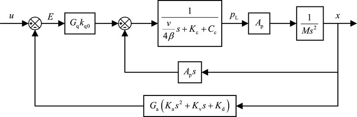
FIGURE 2. Diagram of the three-parameter closed-loop control system transfer function.

Equation 4 represents the closed-loop transfer function of the shaking table’s three-parameter system transfer function diagram.

$\frac{x}{u}=\frac{1}{K_{\mathrm{d}0}{A}_{\mathrm{d}}^{\prime }{G}_{\mathrm{a}}}\frac{1}{\frac{1}{k_{\mathrm{v}}^{\prime }{G}_{\mathrm{q}}{G}_{\mathrm{a}}}\left(\frac{s^3}{n_0^2}+\frac{2D_{0}s}{n_0}+s\right)+\frac{K_{\mathrm{a}0}{A}_{\mathrm{a}}^{\prime }}{K_{\mathrm{d}0}{A}_{\mathrm{d}}^{\prime }}{s}^2+\frac{K_{\mathrm{v}0}{A}_{\mathrm{v}}^{\prime }}{K_{\mathrm{d}0}{A}_{\mathrm{d}}^{\prime }}s+1}(4)$

Where $u$ is the driving signal; $K_{\mathrm{d}0}$, $K_{\mathrm{v}0}$, $K_{\mathrm{a}0}$ are the feedback normalized sensitivity coefficients; ${A_{\mathrm{d}}}^{\prime }$, ${A_{\mathrm{v}}}^{\prime }$, ${A_{\mathrm{a}}}^{\prime }$ are the feedback gains; $G_{\mathrm{a}}$ is the transfer function considering the influence of sensor. $G_{\mathrm{q}}$ is the transfer function considering the influence of the servo valve. where,

$\left\{\begin{array}{l}{G}_{\mathrm{a}}=\frac{1}{\frac{s^2}{n_{\mathrm{a}}^2}+\frac{2D_{\mathrm{a}}s}{n_{\mathrm{a}}}+1}\\ G_{\mathrm{q}}=\frac{1}{\frac{s^2}{n_{\mathrm{q}}^2}+\frac{2D_{\mathrm{q}}s}{n_{\mathrm{q}}}+1}\end{array}\right.(5)$

Where, $n_{\mathrm{a}}$, $n_{\mathrm{q}}$ is the intrinsic frequency of the second-order system; $D_{\mathrm{a}}$, $D_{\mathrm{q}}$ is the intrinsic damping ratio of the second-order system.

Similarly, when Jerk, acceleration, velocity, and displacement feedback are introduced into the shaking table open-loop system, the transfer function block diagram can be obtained as shown in Figure 3. LI Xiaojun et al. [7] In order to expand the effective frequency bandwidth and reduce the resonance frequency of the oil column to achieve the purpose of enhancing the frequency response characteristics of the shaking table. Figure 1 depicts the schematic structure of the multi-variate controller (MVC). In the figure, on the basis of the three-parameter controller (TVC), the red part represents the feed-forward and feedback links with the introduction of Jerk (acceleration derivative). In the parameter gain selection, manual adjustment of parameters is chosen, which leads to a long time consuming to rectify the parameters.

FIGURE 3

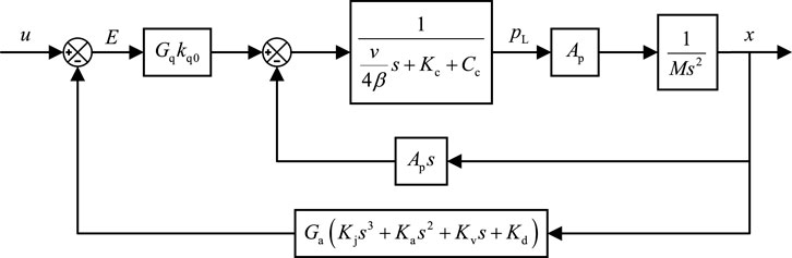
FIGURE 3. Diagram of multi-variable control system transfer function.

Extending Figure 2, a block diagram of the transfer function of the multi-variate controller (MVC) can be obtained, as shown in.

The system’s corresponding transfer function diagram under the shaking table’s multi-variate control is shown in Eq. 6.

$\frac{x}{u}=\frac{1}{K_{\mathrm{d}0}{A}_{\mathrm{d}}^{\prime }{G}_{\mathrm{a}}}\frac{1}{\frac{1}{k_{\mathrm{v}}^{\prime }{G}_{\mathrm{q}}{G}_{\mathrm{a}}}\left(\frac{s^3}{n_0^2}+\frac{2D_{0}s}{n_0}+s\right)+\left(\frac{K_{\mathrm{j}0}{A}_{\mathrm{j}}^{\prime }}{K_{\mathrm{j}0}{A}_{\mathrm{d}}^{\prime }}{s}^3+\frac{K_{\mathrm{a}0}{A}_{\mathrm{a}}^{\prime }}{K_{\mathrm{d}0}{A}_{\mathrm{d}}^{\prime }}{s}^2+\frac{K_{\mathrm{v}0}{A}_{\mathrm{v}}^{\prime }}{K_{\mathrm{d}0}{A}_{\mathrm{d}}^{\prime }}s+1\right)}(6)$

Where $K_{\mathrm{j}0}$ is the jerk feedback normalized sensitivity; $A_j^{\prime }$ is the jerk feedback gain.

The three-variable controller (TVC) and the multi-variable controller (MVC) are analyzed in the frequency domain to obtain Figure 4.

FIGURE 4

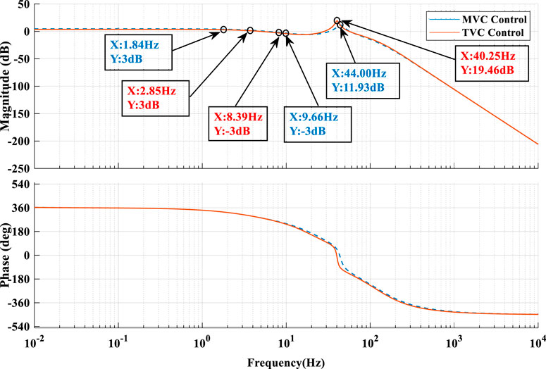
FIGURE 4. Frequency response characteristic curve of the system under TVC control and MVC control.

In Figure 4, the effective frequency bandwidth of the system is between 2.85 Hz and 8.39 Hz when the theoretical parameters are used for the three-variable controller (TVC); the peak of the oil column resonance peak is 19.46 dB at a frequency of 40.25 Hz. While the effective bandwidth of the system is in the range of 1.84 Hz–9.66 Hz when the theoretical parameter control is used in the multi-parameter controller; the peak value of the oil column resonance peak is 11.93 dB when the frequency is 44.00 Hz. It is obvious that, using the theoretical parameters at the same time, the multi-variable controller (MVC) has a better ability to expand the frequency bandwidth than the three-variable controller (TVC), which delays the position where the oil column resonance appears and reduces the peak of the oil column resonance peak.

The study presented in Figure 4 demonstrates that when subjected to theoretical parameter values controlled by several parameters, the resonant frequency of the oil column in the system drops. Additionally, the adequate service bandwidth of the system grows while the resonant peak diminishes. Nevertheless, the resonant peak remains, rendering it inadequate to fulfill the project’s application prerequisites. The present study uses Matlab/Simulink to simulate the shaking table system. The analysis focuses on the implementation of multi-parameter control techniques.

3 Simulation analysis of shaking table under multi-parameter control

The seismic simulation shaking table at Xinyang Normal University was selected as the subject of investigation. The input signals are selected as sine signals, EI-Centro waves, Kobe waves and artificial waves, taking EI-Centro waves as an example. To construct the simulation model of the seismic simulation shaking table, Matlab/Simulink was employed. Subsequently, a thorough analysis was conducted on the simulation results. Table 1 displays the pertinent performance metrics associated with the shaking table. The Matlab/Simulink model of the shaking table is constructed using three-parameter and multi-parameter theoretical parameters for control purposes. Subsequently, separate simulation analyses are conducted.

TABLE 1

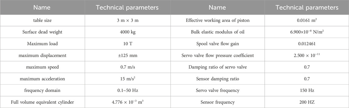
TABLE 1. The parameters of the shaking table.

The reference signal is set as a displacement sinusoidal signal with amplitude of 0.01 m and frequency of 1 Hz, and the simulation results are shown in Figure 5. The correlation coefficient (CC), root mean square error (RMSE) and mean absolute error (MAE) [17–19] of the tracked signals are summarized in Supplementary Table S1. The results in Figure 5 show that the waveforms of acceleration, velocity, and displacement tracking signals under MVC control are more similar with smaller root mean square error (RMSE) and mean absolute error (MAE) compared to those under TVC control.

FIGURE 5

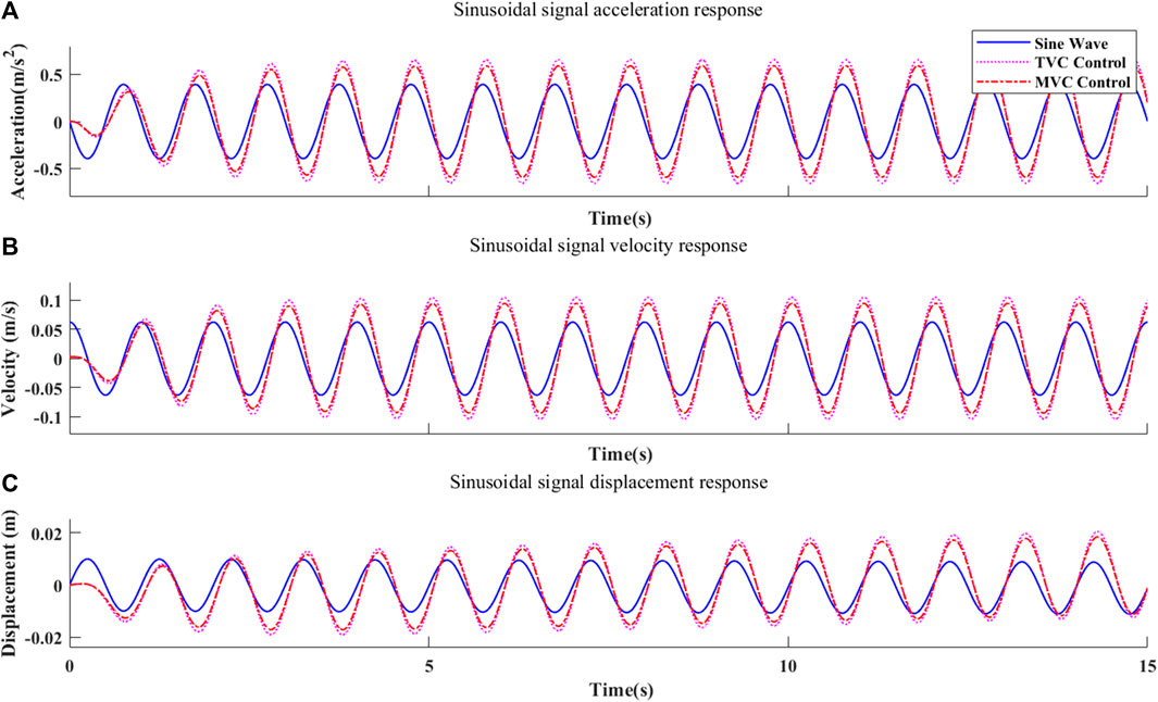
FIGURE 5. Time domain simulation results for sinusoidal signals.

Taking the EI-Centro wave as an example, the shaking table model is built on MatLab/Simulink under the control of TVC theoretical parameters and analyzed by time domain simulation. The simulation results are presented in Figure 6, which depicts the time domain, and Figure 7, which illustrates the frequency domain.

FIGURE 6

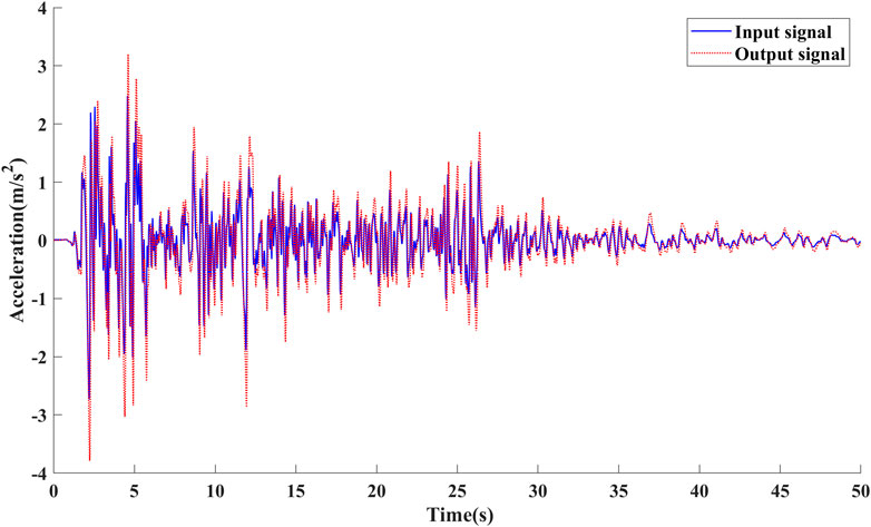
FIGURE 6. Time domain results of the three-variable control (TVC) system simulation.

FIGURE 7

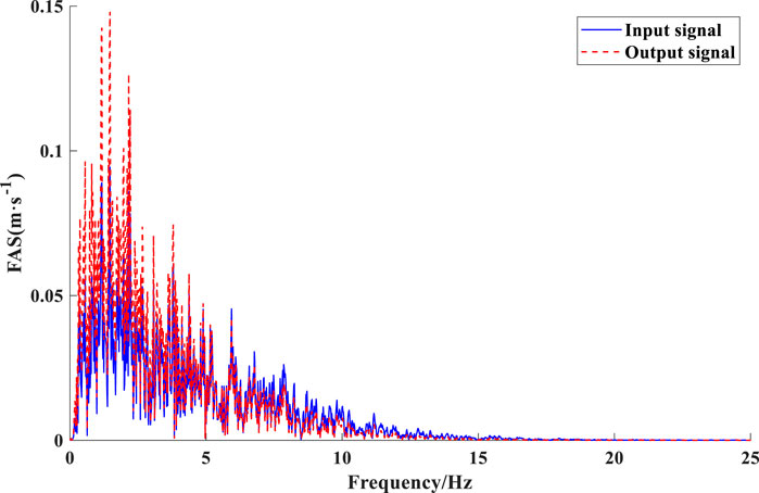
FIGURE 7. Frequency-domain results of three-variable control (TVC) system simulation.

According to the analysis in Figure 6, under the control of the three-parameter theoretical parameter values of the shaking table, the system input and output waveform reproduction accurateness is low, with the calculated CC of 0.6879, the RMSE of 0.464, and the MAE of 0.2971. The results in Figure 7 show that within 0∼5 Hz, the acceleration Fourier amplitude spectrum does not match with the expected value and the amplitude error is large; within 5–10 Hz, the acceleration Fourier amplitude spectrum basically matches with the expected value.

Likewise, the shaking table model is analyzed by time-domain simulation under the control of MVC theoretical parameters using the EI-Centro wave as an example. The simulation results in the time domain are presented in Figure 8, while the simulation results in the frequency domain are displayed in Figure 9.

FIGURE 8

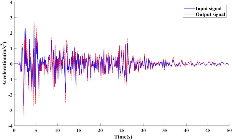
FIGURE 8. Frequency-domain results of multi-variable control (MVC) system simulation.

FIGURE 9

FIGURE 9. Frequency-domain results of multi-variable control (MVC) system simulation.

According to the analysis of Figure 8, under the control of MVC theoretical parameters, the CC of the shape of the shaker acceleration response wave is 0.7011, the RMSE is 0.3869, and the MAE is 0.2789. The results in Figure 9 show that the acceleration Fourier amplitude spectrum still does not match the expected value within 0∼5 Hz, but the amplitude is reduced. The analysis may be caused by reducing the resonance frequency of the system oil column, which is consistent with the results of Figure 4.

The shaking table response characteristics under TVC control and MAC control are summarized in Supplementary Table S2 using three seismic waves as input signals. Compared to the theoretical parametric control of the shaker TVC, the results were not satisfactory, although a small increase in CC and a decrease in RMSE and MAE were achieved with the theoretical parametric control of the MVC.

In order to more visually show the difference between the input signals and the response of the table, three seismic wave signals were used as input signals and compared to the data collected by the accelerometers on the table. It is important to note that this test uses a three-parameter controller (TVC), which provides a side-by-side view of the control of the shaking table. Figure 10 reflects the real relationship between the initial input signals and the table response. Table 1 summarizes the evaluation metrics for the initial signal and table response, including correlation coefficient (CC), root mean square error (RMSE), and mean absolute error (MAE).

FIGURE 10

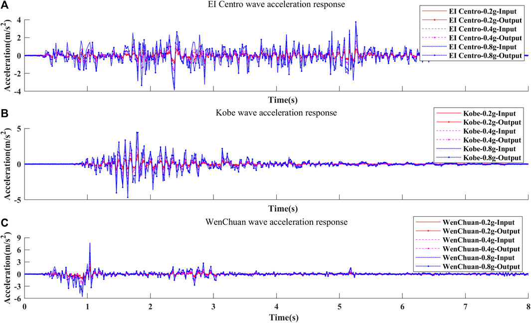
FIGURE 10. Initial Input Signal vs. Test Bench Response.

In shaking table tests, the larger the peak acceleration input signal, the larger the correlation coefficient (CC) of the table response, but the same leads to an increase in the root-mean-square error (RMSE) and mean absolute error (MAE). The increase in RMSE and MAE is within acceptable limits with respect to the choice of TVC or MVC controller. In the case of the EI Centro wave, for example, the mean value of the correlation coefficient (CC) of the true values of the table response is 0.6155, which is similar to the modeled values in Supplementary Table S2, with a relative error of 11.8%; the root-mean-square error (RMSE) and the mean absolute error (MAE) vary considerably, with an order-of-magnitude difference of 1 between the true values and the modeled values.

In summary, the MVC controller performs better than the TVC controller. In order to improve the system frequency response characteristics and waveform reproduction accuracy of the shaking table. For this purpose, a BP neural network is used in the following to form a new controller BP-MVC controller in combination with a multi-variable controller (MVC).

4 Multi—parameter identification of shaking table based on BP network

4.1 Construction of BP neural network

BP (Back Propagation) neural network is a one-way multi-layer feedforward neural network using an error back propagation training procedure, often consisting of the input, hidden, and output layers [20]. The fundamental learning principle employed by the BP algorithm is the method of gradient descent, which aims to maximize the decrease of the gradient. The backpropagation process involves iteratively adjusting the weights and thresholds of a neural network to reduce the sum of squared errors between the network’s predicted output and the desired output.

The input layer of the neural network consisted of eight parameters associated with the shaking table. The nodes in the hidden layer were determined based on Eq. 7 [21]. The researchers discovered that the most effective configuration for the hidden layer consisted of five nodes [22]. They then utilized the measured values of the identified signals as the output layer to develop a neural network model with a network structure of 3–5–8 Figure 11 illustrates a schematic of the flow of the BP neural network.

$i=\sqrt{j+k}+a(7)$

FIGURE 11

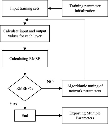
FIGURE 11. Schematic diagram of BP neural network system structure [20].

Let j represent the cardinality of nodes in the input layer, k denote the cardinality of nodes in the output layer, and a symbolize a constant ranging from 0 to 10.

Equation 8 depicts the input-output formula of the input layer in the backpropagation neural network.

$O_{\mathrm{j}}^{\left(1\right)}=x\left(j\right),j=1,2...M(8)$

Where O_j⁽¹⁾ is the input of the jth node of the input layer, j is the node number of the input layer, and M is the number of input variables, which depends on the complexity of the vibration table control system. In this paper, M = 3.

The input and output of the hidden layer of the neural network are shown in Eq. 9.

$\left\{\begin{array}{l}{\text{net}}_{\mathrm{i}}^{\left(2\right)}\left(k\right)={\displaystyle \sum _{j=1}^M}{w}_{\text{ij}}^{\left(2\right)}{O}_{\mathrm{j}}^{\left(1\right)}\\ O_{\mathrm{i}}^{\left(2\right)}\left(k\right)=f\left({\text{net}}_{\mathrm{i}}^{\left(2\right)}\left(k\right)\right),i=1,2,...,Q\end{array}\right.(9)$

Where net_i⁽²⁾ is the input of the ith node of the hidden layer; i is the number of the neuron node of the hidden layer; w_ij⁽²⁾ is the connection weight between the neuron j of the input layer and the neuron i of the hidden layer; O_i⁽²⁾ is the output of the ith node of the neuron of the hidden layer; f (·) is the activation function of the hidden layer. The activation function of hidden layer neurons is the Sigmoid function, as shown in Eq. 10.

$f\left(x\right)=\frac{e^x-e^{-x}}{e^x+e^{-x}}(10)$

The input and output of the network output layer are shown in Eq. 11.

$\left\{\begin{array}{l}{\text{net}}_{\mathrm{k}}^{\left(3\right)}\left(k\right)={\displaystyle \sum _{i=1}^Q}{w}_{\text{ij}}^{\left(3\right)}{O}_{\mathrm{i}}^{\left(2\right)}\left(k\right)\\ O_{\mathrm{i}}^{\left(3\right)}\left(k\right)=g\left[{\text{net}}_{\mathrm{i}}^{\left(3\right)}\left(k\right)\right]\\ O_1^{\left(3\right)}\left(k\right)=y\end{array}\right.(11)$

Where net_k⁽³⁾ is the input of the kth node of the output layer, k is the number of nodes of the output layer, O_k⁽³⁾ is the output of the kth node of the neuron of the output layer, and g (·) is the activation function of the output layer.

The output layer corresponds to the signal generated by the system identification model of the shaking table in response to input stimuli. The activation function employed in the output layer is linear, specifically referred to as Purelin, as depicted in Eq. 12.

$g\left(x\right)=x(12)$

Take the performance index and error functions as shown in Eq. 13.

$\left\{\begin{array}{l}J\left(k\right)=\frac{1}{2}{\left(rin\left(k\right)-yout\left(k\right)\right)}^2\\ Error\left(k\right)=rin\left(k\right)-yout\left(k\right)\end{array}\right.(13)$

Where rin (k) is the reference input at the current moment; yout (k) is the output of the current system time.

Calculate the control quantity u (k), as shown in Eq. 14.

$u\left(k\right)=Aa\cdot w11+Av\cdot w12+Ad\cdot w13+Aj\cdot w14+Aaf\cdot w15+Avf\cdot w16+Adf\cdot w17+Ajf\cdot w18(14)$

Adjust the weight coefficient of the network according to the method of the fastest gradient descent. In order to achieve progressive convergence, it is necessary to make adjustments in the opposite direction of the gradient change of the J (k) function. The formula for correcting the weight coefficient of each neuron in the output layer is presented in Eq. 15.

$\left\{\begin{array}{l}\Delta \omega \text{ki}=-\eta \frac{\partial J\left(k\right)}{\partial \omega \text{ki}}=\eta {\delta }_{\mathrm{k}}^{\left(3\right)}\left(k\right)O_{\mathrm{i}}^{\left(2\right)}\left(k\right)\\ {\delta }_{\mathrm{k}}^{\left(3\right)}\left(k\right)=-\frac{\partial J\left(k\right)}{\partial {\text{net}}_{\mathrm{k}}^{\left(3\right)}\left(k\right)}\end{array}\right.(15)$

Where η is the learning rate, η > 0; Δw is the weight adjustment, and δ_k is the local gradient.

Equation 16 provides the adjusted formula for the weight coefficient of each neuron in the hidden layer, as derived from the gradient approach.

$\left\{\begin{array}{l}\Delta \omega \text{ij}=-\eta \frac{\partial J\left(k\right)}{\partial \omega \text{ij}}=\eta {\delta }_{\mathrm{i}}^{\left(3\right)}\left(k\right)O_{\mathrm{j}}^{\left(2\right)}\left(k\right)\\ {\delta }_{\mathrm{i}}^{\left(2\right)}\left(k\right)=-\frac{\partial J\left(k\right)}{\partial {\text{net}}_{\mathrm{j}}^{\left(2\right)}\left(k\right)}\end{array}\right.(16)$

The weight correction formula for the hidden and output layers is depicted in Eq. 17.

$w\left(k\right)=w\left(k-1\right)+\Delta w\left(k\right)(17)$

4.2 Multi—parameter identification of shaking table based on BP network

Figure 12 illustrates the structural model of the multi-parameter parameter identification system for seismic simulation shaking tables, which is based on the BP neural network.

FIGURE 12

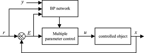
FIGURE 12. Schematic diagram of system structure.

The algorithmic process for seismic simulation using a shaking table and a BP neural network is outlined as follows [23–25]:

(1) Initialize, determine the network topology structure of the BP neural network, give all the weighted coefficients and thresholds, and select the learning rate.

(2) The input and output of neurons in each neural network layer are determined. The eight input parameters are $A_{\mathrm{a}}$, $A_{\mathrm{v}}$, $A_{\mathrm{d}}$, $A_{\mathrm{j}}$, $A_{\text{af}}$, $A_{\text{vf}}$, $A_{\text{df}}$, and $A_{\text{jf}}$.

(3) The input and output of neurons at each layer of the fundamental neural network are calculated. The output is a parameter, that is, the output signal of the shaking table identification system.

(4) Online learning of neural network, online weight adjustment, and finally achieving $A_{\mathrm{a}}$, $A_{\mathrm{v}}$, $A_{\mathrm{d}}$, $A_{\mathrm{j}}$; Parameter optimization of $A_{\text{af}}$, $A_{\text{vf}}$, $A_{\text{df}}$, and $A_{\text{jf}}$.

(5) Set k = k + 1 and return to step (3) until the shaking table system model error is minimal and meets the requirements.

4.3 Experimental simulation analysis

Frequency domain analysis of the stabilized system leads to Figure 13. In the figure, using the BP-MVC controller, the effective frequency bandwidth of the system ranges from 0.014 Hz to 63.20 Hz, with no obvious oil column resonance peaks.

FIGURE 13

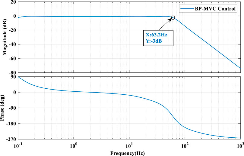
FIGURE 13. Frequency response characteristic curve of the system under BP-MVC control.

The Matlab/Simulink model is developed to implement multi-parameter control of a seismic simulation shaking table using a BP neural network. With the same signal input and the parameters adjusted by BP neural network, the model output response is as follows:

The output signals (acceleration, velocity and displacement) are plotted versus the real situation for sinusoidal signals in Figure 14. CC, RMSE and MAE are summarized in Supplementary Table S4. It can be seen that the tracking response curves match the real values after the BP neural network identification, both for the acceleration tracking signal and the velocity and displacement tracking signals. Compared with the MVC control, the BP-MVC control makes the CC obtain a substantial improvement. Especially, the CC of the displacement signal is improved from 0.8947 to 0.9981. In addition, the RMSE and MAE are also decreased significantly. In particular, when tracking the displacement signal, the RMSE drops to 0.0006. When the input is a sinusoidal signal, the sources of error for the MVC control are the amplitude and phase differences.

FIGURE 14

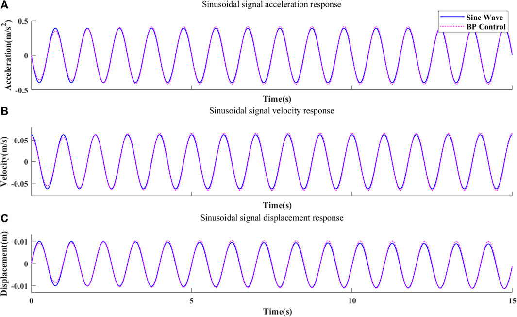
FIGURE 14. Time domain simulation results for sinusoidal signals.

According to the analysis in Figure 15, the waveform recurrence accuracy of the shaking table system is significantly improved by the multi-parameter control based on BP network adjustment. The CC is 0.9960, the RMSE is 0.0380, and the MAE is 0.2448 when the EI-Centro wave is used as the input signal; the results in Figure 16 show that the spectral amplitude overlap is significantly improved.

FIGURE 15

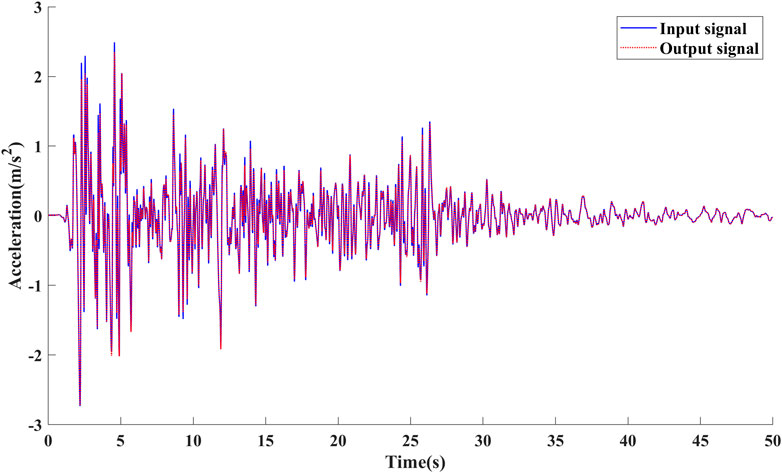
FIGURE 15. Time domain simulation diagram of the system with optimized parameters.

FIGURE 16

FIGURE 16. Simulation diagram of system frequency domain with optimized parameters.

Supplementary Table S5 summarizes the response characteristics of the shaker under BP-MVC control using three seismic waves as input signals. It can be seen that the BP-MVC control achieves the tracking of the shaker signal by increasing the CC and decreasing the RMSE and MAE based on the MVC control. The MVC control has different effects on the tracking of the three seismic waves, in which the CC of the artificial wave is as low as 0.4928, while the CC of each seismic wave under the BP-MVC control is above 0.996.

Figure 17 plots the variation of the initial multiparametric theoretical values when the input signal is an EI Centro wave. It can be seen that with 8 initial inputs, the parameters stabilize within about 25 s after learning by the BP neural network. Compared with the three-parameter theoretical parameter control (TVC) or multi-parameter theoretical parameter control (MVC), the BP neural network control can achieve convergence quickly, and the control error of the parameters is controlled within ${10}^{-5}\sim {10}^{-8}$.

FIGURE 17

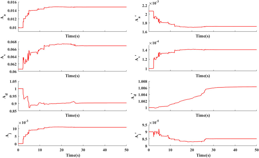
FIGURE 17. Schematic diagram of multi-parameter change under BP neural network learning.

5 Conclusion and discussion

This study focuses on the intelligent control of a seismic simulation shaking table. Specifically, it explores the implementation of acceleration control using a three-parameter control approach. The aim is to develop a seismic simulation shaking table incorporating multi-parameter control techniques. Through theoretical research and simulation analysis, the BP-MVC controller expands the frequency bandwidth of the system, reduces the resonance peak of the oil column on the basis of MVC, and improves the system frequency response characteristics of the shaking table. This study presents a multi-parameter control model for seismic simulation shaking table using the BP neural network under the framework of multi-parameter control. The model is meant to identify significant parameters online and provide a set of optimization parameters. The objective is to enhance the correlation of shaking table waveform. The results from the shaking table system simulation, utilizing optimized parameters, demonstrate that the suggested algorithm substantially improves waveform reproduction accuracy. This improvement aligns with the engineering requirements and serves as evidence for the efficacy of the proposed algorithm. This study focuses on implementing a single degree of freedom (DOF) seismic simulation shaker. The findings of this research can potentially be used for more complex systems such as the tri-axial and six degrees of freedom seismic simulation shaking table.

Data availability statement

The raw data supporting the conclusion of this article will be made available by the authors, without undue reservation.

Author contributions

CG: Conceptualization, Funding acquisition, Writing–original draft. CL: Writing–original draft. MQ: Data curation, Visualization, Writing–review and editing. YY: Data curation, Visualization, Writing–review and editing. ZY: Visualization, Writing–review and editing.

Funding

The author(s) declare financial support was received for the research, authorship, and/or publication of this article. This work was supported by the Henan Provincial Department of Science and Technology (No. 212300410234) and Xinyang Normal University Nos. 2022KYJJ088 and 2022KYJJ090.

Acknowledgments

The author thanks the teachers and classmates of the team for collecting the experimental data.

Conflict of interest

The authors declare that the research was conducted in the absence of any commercial or financial relationships that could be construed as a potential conflict of interest.

Publisher’s note

All claims expressed in this article are solely those of the authors and do not necessarily represent those of their affiliated organizations, or those of the publisher, the editors and the reviewers. Any product that may be evaluated in this article, or claim that may be made by its manufacturer, is not guaranteed or endorsed by the publisher.

Supplementary material

The Supplementary Material for this article can be found online at: https://www.frontiersin.org/articles/10.3389/fphy.2024.1309029/full#supplementary-material

References

1. Gao C, Yuan X. Development of the shaking table and array system Technology in China. Adv Civil Eng (2019) 2019:1–10. doi:10.1155/2019/8167684

CrossRef Full Text | Google Scholar

2. Zhao J, Dong J, Sun X, Xu J, Zhao L, Li W. Development and teaching application of electro-hydraulic servo shaking table. Exp Tech Manag (2021) 38:172–6. doi:10.16791/j.cnki.sjg.2021.10.032

CrossRef Full Text | Google Scholar

3. Ceresa P, Brezzi F, Calvi GM, Pinho R. Analytical modelling of a large-scale dynamic testing facility. Earthquake Eng Struct Dyn (2012) 41:255–77. doi:10.1002/eqe.1128

CrossRef Full Text | Google Scholar

4. Tagawa Y, Kajiwara K. Controller development for the E-Defense shaking table. Proc Inst Mech Eng J Syst Control Eng (2007) 221:171–81. doi:10.1243/09596518JSCE331

CrossRef Full Text | Google Scholar

5. Luan Q, Chen Z, Xu J, He H. Three-variable control technique for a seismic analog shaking table. J vibration Shock (2014) 33:54–60. doi:10.13465/j.cnki.jvs.2014.08.010

CrossRef Full Text | Google Scholar

6. Cui W, Wang S, Ren W. An improved three-parameter control of earthquake shaking table. Chin Hydraulics Pneumatics (2012) 144–6. doi:10.3969/j.issn.1000-4858.2012.11.048

CrossRef Full Text | Google Scholar

7. Li X, Li F, Ji J, Wang J. A new control Technology of shaking table based on the jerk. Adv Eng Sci (2018) 50:64–72. doi:10.15961/j.jsuese.201800370

CrossRef Full Text | Google Scholar

8. Ji J, Sun L, Zhan P, Li N, Zhang S. Control parameters auto-tuning methods of shaking table based on expert experiences. Tech Earthquake Disaster Prev (2014) 9:882–90. doi:10.11899/zzfy20140416

CrossRef Full Text | Google Scholar

9. Gao C, Wang J, Zhang Y, Yuan X. The influence on the control performance caused by load characteristic in the shaking table. J Xinyang Normal University (Natural Sci Edition) (2022) 35:145–50. doi:10.3969/j.issn.1003-0972.2022.01.025

CrossRef Full Text | Google Scholar

10. Yu S, Liu X, Wang J, Liu D, Jin Y. Application of BP neural networks in electro-hydraulic shaking table control system. Chin Hydraulics Pneumatics (2008) 53–5. doi:10.3969/j.issn.1008-0813.2022.09.003

CrossRef Full Text | Google Scholar

11. Mu H, Luo Y, Du W, Deng H. Simulation research on synchronous control of double hydraulic cylinder based on BP-PID. Hydraulics Pneumatics & Seals (2022) 42:14–31.

Google Scholar

12. Zhang F, Zhou H, Zhang B, Song W, Wang T. Real-Time Iterative Control Method Research of Shaking Table. Eng Mech (2022) 1–13. doi:10.6052/j.issn.1000-4750.2022.03.0265

CrossRef Full Text | Google Scholar

13. Ji J, Hu Z, Yang S. Closed-loop control method of seismic simulation shaking table based on LSTM. Earthquake Eng Eng Dyn (2022) 42:63–9. doi:10.13197/j.eeed.2022.0507

CrossRef Full Text | Google Scholar

14. Liu H, Wang hu, Wang Y. PID control of marine pressure simulator based on BP neural network. Instrumentation and Equipments (2019) 07:155–63. doi:10.12677/IaE.2019.73022

CrossRef Full Text | Google Scholar

15. Xie L, Qin L. Fractional order PIλDμ control based on neural network optimization algorithm. J Nanjing Univ Sci Tech (2021) 45:515–20. doi:10.14177/j.cnki.32-1397n.2021.45.04.017

CrossRef Full Text | Google Scholar

16. Yao J, Dietz M, Xiao R, Yu H, Wang T, Yue D. An overview of control schemes for hydraulic shaking tables. J Vibration Control (2016) 22:2807–23. doi:10.1177/1077546314549589

CrossRef Full Text | Google Scholar

17. Wang L, Zhao Y, Liu J. A Kriging-based decoupled non-probability reliability-based design optimization scheme for piezoelectric PID control systems. Mech Syst Signal Process (2023) 203:110714. doi:10.1016/j.ymssp.2023.110714

CrossRef Full Text | Google Scholar

18. Liu Y, Wang L. Multiobjective-clustering-based optimal heterogeneous sensor placement method for thermo-mechanical load identification. Int J Mech Sci (2023) 253:108369. doi:10.1016/j.ijmecsci.2023.108369

CrossRef Full Text | Google Scholar

19. Liu Y, Wang L. A robust-based configuration design method of piezoelectric materials for mechanical load identification considering structural vibration suppression. Comp Methods Appl Mech Eng (2023) 410:115998. doi:10.1016/j.cma.2023.115998

CrossRef Full Text | Google Scholar

20. Yousefi H, Hirvonen M, Handroos H, Soleymani A. Application of neural network in suppressing mechanical vibration of a permanent magnet linear motor. Control Eng Pract (2008) 16:787–97. doi:10.1016/j.conengprac.2007.08.003

CrossRef Full Text | Google Scholar

21. Zhang G, Liu C, Men T. Research on data mining Technology based on association rules algorithm. In: 2019 IEEE 8th Joint International Information Technology and Artificial Intelligence Conference (ITAIC); May 24-26, 2019; Chongqing China (2019). p. 526–30. doi:10.1109/ITAIC.2019.8785788

CrossRef Full Text | Google Scholar

22. Yao J, Wang T, Wan Z, Chen S, Niu Q, Zhang L. Identification of acceleration harmonics for a hydraulic shaking table by using hopfield neural network. Scientia Iranica (2017) 0:0. doi:10.24200/sci.2017.4318

CrossRef Full Text | Google Scholar

23. Chunhua Ga. O, Jieqiong W, Yanping Y, Mengyuan QIN. Parameter optimization of shaking table based on later random and nonlinear dynamic particle swarm optimization. xysfxyxb (2023) 36:137–43. doi:10.3969/j.issn.1003-0972.2023.01.023

CrossRef Full Text | Google Scholar

24. Wenqiang MA, Jiuting W. Macro-and meso-failure characteristics and energy evolution of granite under uniaxial compression. Geotechnical Geol Eng (2023) 36:314–20. doi:10.3969/j.issn.1003-0972.2023.02.025

CrossRef Full Text | Google Scholar

25. Chao FU, Qifang Ya. N, Zhichao LI, Chaoyang DU. Bending deformation of a simple-supported viscoelastic timoshenko beam with switching cracks. Adv Civil Eng (2023) 36:144–9. doi:10.3969/j.issn.1003-0972.2023.01.024

CrossRef Full Text | Google Scholar