Merging single-track location Elastographic imaging with the frequency shift method improves shear wave attenuation measurements

Introduction

Characterizing tissue mechanical properties is crucial as disease progression is associated with changes in tissue mechanical properties [1–3]. Shear wave elastography (SWE) visualizes the viscoelastic properties (elasticity and viscosity) within soft tissue from the measured shear modulus [4]. Researchers have used SWE to demonstrate that elasticity can stage liver fibrosis [5] and differentiate malignant from benign breast tumors [6]. Other mechanical parameters have also been used to diagnose disease [7,8]. For example, using magnetic resonance elastography, researchers have demonstrated that multiple sclerosis reduces both elasticity and viscosity of the brain [9]. Researchers have demonstrated that viscosity is more sensitive to liver damage (steatosis) than elasticity [10,11]. Furthermore, liver inflammation also resulted in elevated viscosity [12,13]. However, quantifying viscosity is challenging due to the lack of consensus on the appropriate rheological model, in addition to the geometric spreading of the shear wave [14]. Consequently, developing methods to measure soft tissues’ viscous properties more accurately remains an active area of research.

Measuring viscosity through rheological models can be useful; however, selecting the correct model for a specific clinical application can be challenging due to the numerous options available. Researchers have used the Kelvin-Voigt and Kelvin-Voigt fractional derivative (KVFD) models to characterize the viscous behavior of tissue [14–16]. Chen and colleagues [15] developed a method that estimates viscosity by fitting the shear wave spectrum to the Kelvin-Voigt model. The viscoelastic parameters measured from the shear wave spectrum were comparable to measurements made from independent mechanical testing, demonstrating the potential application of their technique. Hossain et al. developed viscoelastic response (VisR) which provides relative elasticity and relative viscosity using the acoustic radiation force impulse fitted to the mass-spring damper model [17].

Alternatively, researchers proposed techniques which estimate viscoelasticity without using a rheological model. Vappou et al. proposed estimating the complex shear modulus from the properties of the propagating shear wave and the phase shift between the shear stress and strain applied using harmonic motion imaging [18]. Researchers have also proposed using group shear wave speed (SWS) and its derivatives [19] to characterize viscosity. Their approach was more robust than the shear wave spectrum-based method and overcame the challenge of selecting the appropriate model. Hossain et al. demonstrated that multi frequency oscillation-SWE could improve the estimation of phase velocity for higher frequencies [20]. Amador et al. estimated viscoelasticity from acoustic radiation force creep and shear wave dispersion [21]. Other technique provide information about the viscoelastic properties from relaxation time constant after acoustic radiation force impulse [22]. Kijanka et al. proposed local phase velocity based imaging (LPVI) to reconstruct phase velocity maps using sequential pushes at both sides of the imaging medium [23]. Kazemirad and colleagues [24] developed a model-free technique that measures both storage (related to elasticity) and loss (related to viscosity) moduli by assuming that shear wavefronts are cylindrical, which is rarely the case in soft tissues. An alternate approach is to measure the shear wave attenuation coefficient by observing the decrease in amplitude as shear waves travel through the tissue. To ensure precise estimates with this method, the effects of geometric spreading and the shape of the shear wave front must be considered. In general, the wavefront consists of cylindrical and planar waves. Therefore, researchers typically assume shear waves are either cylindrical or planar [25,26] when computing the attenuation coefficient. For example, Nenadic and colleagues [27] developed a promising technique called attenuation measuring ultrasound shear wave elastography (AMUSE), which includes a factor $\sqrt{x}$ (with x being the lateral distance the wave has traveled) when computing the attenuation coefficient from cylindrical shear wavefronts. AMUSE performed well in post-transplant liver patients. However, like other viscosity estimation techniques [15,27,28], AMUSE assumes homogenous tissue structures which is not the case in complex heterogeneous tissues such as pancreatic cancer, where reflections and diffractions impede the propagation of shear waves, resulting in inaccurate attenuation estimates. Consequently, new methods are needed to measure the viscosity of heterogeneous tissues.

The frequency shift (FS) method offers a new approach for estimating shear wave attenuation which could be used to estimate the viscosity of heterogeneous tissues. This method was developed to measure the attenuation of seismic waves [29], and recently extended to elastography [30]. The FS method is based on two assumptions. First, that the range of frequencies in shear waves has a Gamma distribution [24,31,32]. Second, geometric spreading is assumed to be frequency-independent [30]. It is generally assumed that the shear wave spectrum generated by an acoustic radiation force has a Gaussian distribution [26,33,34]. However, it has been reported that the Gamma distribution provides a better fit for the shear wave spectrum [30–32]. Another limitation is that shear wave attenuation coefficient maps are typically reconstructed by averaging the shear wave spectrum obtained from multiple depths and lateral positions [30], which is computationally demanding. To address this limitation, Kijanka et al. [32] developed an approach that estimates attenuation coefficient from two points using the FS method. Yazdani et al. [31] recently developed an approach that employs random sample consensus with the FS method, which reduces the effect of noise and outliers. However, like the AMUSE method, the tissue under investigation is also assumed to be homogeneous, which raises doubts concerning its suitability for measuring the attenuation coefficient of heterogeneous tissues such as cancer.

We recently extended the plane wave single-track location shear wave elastography (pSTL) [35] method we previously developed to estimate SWS, to also estimate the attenuation coefficient of heterogeneous tissue, an approach we have called the plane wave single-track location FS method (pSTL-FS). Averaging the attenuation maps generated with different push pairs allows us to compute more reliable estimates of both SWS and attenuation. The goal of this study was to evaluate the effectiveness of pSTL-FS approach in estimating the shear wave attenuation coefficient by fitting the shear wave spectrum to either a Gamma or Gaussian distribution. A secondary goal of this study was to assess the performance of pSTL-FS compared to the AMUSE and standard FS methods with Gamma and Gaussian distributions.

Theory

The FS method has been previously described [30], therefore, this section provides a brief description of the technique. Assuming that $S\left(f\right)$ is the shear wave spectrum at location $x_0$, the shear wave spectrum $V\left(f\right)$ after travelling a distance of $\Delta x$ is given as follows:

$V\left(f\right)=S\left(f\right)\bullet G\left(f,\Delta x\right)\bullet H\left(f,\Delta x\right),(1)$

where $G\left(f,\Delta x\right)$ and $H\left(f,\Delta x\right)$ represent geometric spreading, assumed to be frequency independent, and shear wave attenuation within the medium, respectively. Assuming the attenuation coefficient (${\alpha }_0$) varies linearly with frequency ($f$), then shear wave attenuation is defined as follows [30]:

$H\left(f,\Delta x\right)=e^{-{\alpha }_{0}f\Delta x}(2)$

Assuming a Gamma distribution, the shear wave spectrum is defined as follows [30]:

$S\left(f\right)\propto A\bullet f^{k_0-1}\bullet e^{-f{\beta }_0},(3)$

where $k_0$ and ${\beta }_0$ represent the shape and rate parameters, respectively, of the Gamma distribution, and $A$ is the shear wave amplitude. The shape parameter, $k_0$ is assumed to be constant as the shear waves propagate. Therefore, $Eq.1$ can be expressed as follows:

$V\left(f\right)\propto A\bullet f^{k_0-1}\bullet e^{-f\left({\beta }_0+{\alpha }_0\Delta x\right)},(4)$

$V\left(f\right)$ is approximated with a Gamma distribution of parameters $k_1$ and ${\beta }_1$, which is a function of $S\left(f\right)$ parameters and ${\alpha }_0$ is related to $V\left(f\right)$ and $S\left(f\right)$ parameters as follows:

${\beta }_1={\beta }_0+{\alpha }_0\Delta x(5)$

Calculating the rate parameter over a range of lateral positions, ${\alpha }_0$ is achieved by minimizing the following objective function:

$\left[A,k_0,\beta \left(\Delta x\right)\right]={\mathrm{argmin}}_{A,k_0,\beta \left(\Delta x\right)}{‖V\left(f,\Delta x\right)-S\left(f,x_0\right)‖}_2^2(6)$

Alternatively, the shear wave spectrum $\left(S\left(f\right)\right)$ can also be represented by a Gaussian distribution as follows [33]:

$S\left(f\right)=A\exp \left(-\frac{{\left(f-f_s\right)}^2}{{\sigma }_s^2}\right),(7)$

Where $f_s$ and ${\sigma }_s$ represent the centroid frequency and standard deviation of the shear wave spectrum, respectively. After traveling $\Delta x$, the shear wave spectrum ($\left.V\left(f\right)\right)$ can also be approximated by a Gaussian distribution with a centroid frequency of $f_v$ and a standard deviation of ${\sigma }_v$ as follows:

$V\left(f\right)\approx A\exp \left(-\frac{{\left(f-f_v\right)}^2}{{\sigma }_v^2}\right)(8)$

Substituting Eq. 7 and Eq. 2, into Eq. 1 gives the following relation:

$V\left(f\right)\approx A\mathit{exp}\left(-\left(\frac{{\left(f-f_s\right)}^2+{\alpha }_{0}f\Delta x{\sigma }_s^2}{{\sigma }_s^2}\right)\right)(9)$

$S\left(f\right)$ and $V\left(f\right)$ are related when both spectra have a common standard deviation $\left({\sigma }_v={\sigma }_s\right)$. Hence, the centroid frequency is the only parameter needed for the Gaussian distribution. When ${\sigma }_s$ and ${\sigma }_v$ are equivalent, Eq. 9 becomes:

$V\left(f\right)\approx A\mathit{exp}\left(-\frac{{\left(f-f_v\right)}^2}{{\sigma }_s^2}\right)\mathit{exp}\left(-\frac{Q}{{\sigma }_s^2}\right)(10)$

where:

$f_v=f_s-0.5{\alpha }_0\Delta x{\sigma }_s^2(11)$

and:

$Q=f_s{\alpha }_0\Delta x{\sigma }_s^2-{\left(0.5{\alpha }_0\Delta x{\sigma }_s^2\right)}^2(12)$

Since the shear wave spectra are normalized by $S\left(f\right)$ amplitude, the term $\mathit{exp}\left(-\frac{Q}{{\sigma }_s^2}\right)$ in Eq. 10 is generally ignored [30]. The attenuation coefficient is estimated from Eq. 11 by minimizing Eq.6 at multiple lateral positions.

Materials and methods

Estimating the spatial variation of the attenuation coefficient using the pSTL framework

We extended the pSTL shear wave elastography (pSTL-SWE) method that we previously introduced [35] to also estimate shear wave attenuation. To briefly review how pSTL-SWE estimates SWS, we assume a focused ultrasound beam (the push beam) induces shear waves in the tissue of interest. The arrival time of the resulting shear waves is estimated at a fixed location. A second push beam is transmitted at a different lateral position in the tissue, and the resulting shear wave’s arrival time is measured at the same point as the first push beam. This process is repeated several times at different push beam positions to produce SWS maps as illustrated in Figure 1A. pSTL-SWE’s advantage lies in the use of plane wave imaging for tracking, which enables the synthesis of multiple single-track location shear wave elastography (STL-SWE) data [36] from a single acquisition. Furthermore, creating a composite SWS map from the associated data reduces the impact of random errors and speckle noise on SWS estimates. To estimate the shear wave attenuation coefficient with the pSTL-SWE framework, we applied either a Gaussian (Eqs 7, 8, 11) or a Gamma (Eqs 3–5) probability distribution function (PDF) to the shear wave spectrums generated with two different push beams. The shear wave attenuation coefficient is then computed by applying Eq. 5 to the fitted spectra. Figure 1B shows the push beam pair where the attenuation coefficient was computed for the center point in between the pushes. Both push beams’ positions were shifted laterally by 0.30 mm, and the procedure was repeated, as shown in Figure 1C. The distance between the push pair ($\left.\Delta P\right)$ and the tracking beam was varied to generate attenuation estimates from multiple push pairs.

Figure 1

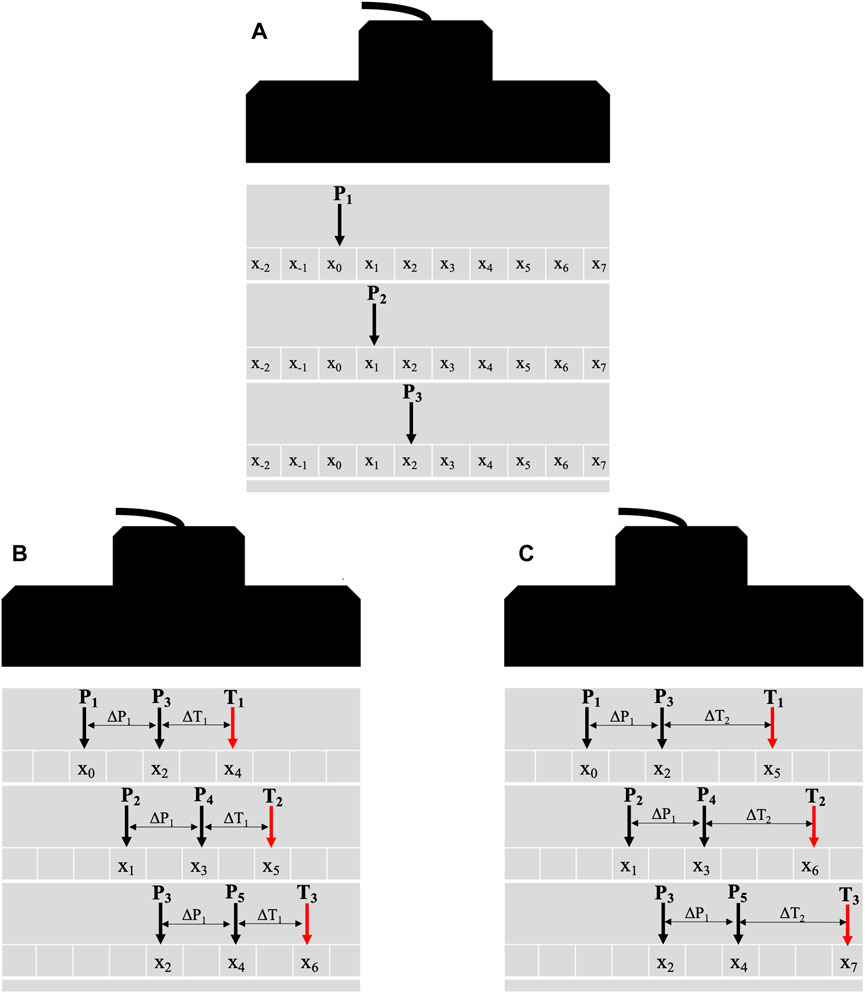
Figure 1. Schematic diagrams illustrating the general principle of the pSTL technique. The technique involves a sequential process of a push followed by tracking across the entire aperture (A) for laterally shifting pushes. The black and red arrows depict the push and tracking beams, respectively. Diagrams (B, C) illustrate the synthesis of multiple datasets using combinations of push and tracking distances. The push beam (P₁), initially positioned at a lateral position x₀, generates a shear wave where plane wave compounding is used to capture its propagation (A). The push beam is laterally shifted, and plane wave compounding is repeated to generate multiple datasets. To reconstruct the attenuation coefficient maps (B, C), the shear waves from push beams P₁ and P₃ (separated by 0.60 mm) are tracked at T₁ (∆T₁ from P₃). The push pair and tracking beam are laterally shifted by 0.30 mm while maintaining the same tracking distance. Once the tracking beam reaches the aperture’s end, the initial push pair (P₁ and P₃) is reused with a new tracking distance ∆T₂. The tracking distance (ΔT) varied between 4 mm and 8.7 mm. This process is repeated with ∆P₁ being set to 0.60 mm, 1.20 mm, and 1.81 mm.

Data acquisition and post processing

We implemented pSTL-FS on a commercially available ultrasound scanner (Vantage 256, Verasonics Inc., Kirkland, WA, United States) equipped with a 11-5v linear transducer (Verasonics Inc., Kirkland, WA, United States). The push beams were focused at depths 5 mm, 10 mm, and 15 mm, with the push duration and frequency set to 150 μs and 5 MHz, respectively. Compounded plane wave imaging was performed immediately after each push with steering angles (−3, −1, 0, 1, 3) and a pulse repetition frequency of 7 kHz. To estimate SWS, we applied a 2D auto-correlation algorithm [37] to beamformed radiofrequency echo data to estimate particle displacement as previously described [35]. Prior to curve fitting in the frequency domain, the particle velocity was calculated by multiplying the particle displacement by frequency. For in vivo studies, a motion gating system was implemented to assure shear wave acquisition was performed in the quiet zone of the breathing cycle [38]. The resulting data underwent bandpass filtering with cutoff frequencies 50 Hz and 1,000 Hz, and median filtering in the slow time dimension. The data acquisition was the same for the phantom and in vivo studies. For the curve fitting, an empirical assessment of the shear wave spectrum demonstrated noise artifacts for frequencies higher than 700. Therefore, we have restricted the fitted shear wave spectrum’s frequency range from 50 Hz to 700 Hz. For the phantom studies, we acquired 10 data sets per phantom to perform statistical analysis on the different acquisitions.

To reduce the computational burden when estimating the attenuation coefficient, all computations were restricted to the central lateral region of the transducer, ranging from 18 mm to 24 mm. The distance between the left-most push beam and the tracking location varied from 4 mm to 8.7 mm in 0.30 mm increments. Additionally, the distance between the push pairs was varied from 0.60 mm to 1.82 mm in 0.60 mm increments. For the standard FS method, an equivalent number of laterally shifted push beams were used to generate multiple attenuation maps which are averaged to a single map. All computations were performed with a 3 mm × 4 mm moving kernel as illustrated in Figure 2E. The particle displacement was averaged vertically (depth dimension), and the distribution parameters, Gamma or Gaussian, were estimated for every lateral position in the kernel. The attenuation coefficient was computed from the gradients of the rate parameter relative to the distance from the starting tracking position (Eq. 6).

Figure 2

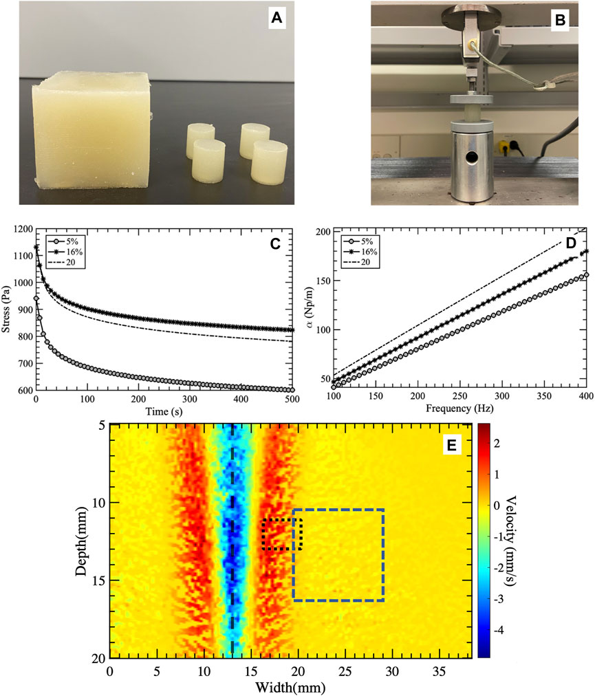
Figure 2. (A) Photograph showing the calibrated cubic and cylindrical phantoms used for ultrasound imaging and mechanical testing, respectively. (B) Experimental setup used to deform the cylindrical phantoms and (C) measure the stress responses over time. The gray circles, black asterisk, and dashed line represent oil percentages of 5%, 16%, and 20%, respectively. The stress relaxation curves were fitted to the Kelvin-Voigt fractional derivative (KVFD) model to extract the model’s parameters. Subplot (D) presents the attenuation curves as a function of frequency used to obtain the attenuation coefficients. Visualization of the shear wave generated by a push beam with the ROI (blue dashed rectangle) selected for techniques comparison (E). The black dashed line shows the lateral position of the push beam. The black dotted rectangle depicts the window used by the FS method to calculate a single attenuation coefficient value over depth and lateral positions. The FS technique uses a sliding window approach to reconstruct the shear wave attenuation coefficient map.

Attenuation measuring ultrasound shear wave elastography technique

We implemented the AMUSE technique as described by Nenadic et al. (Nenadic et al. [39]. To produce the two-dimensional (2D) spatial-temporal map as a function of spatial (k) and temporal (f) frequencies, we computed the 2D Fourier transform of the particle displacement with respect to space (x) and time (s). Calculations were made over various frequencies to determine the full width half maximum (FWHM) of the particle displacement spectrum. The attenuation coefficient (α) was calculated as follows: $\alpha =\text{FWHM}\bullet \pi /\sqrt{x}$. We fitted the attenuation slope computed at various frequencies to a linear function to obtain the attenuation coefficient as described in the original work [27].

Phantom fabrication

Three homogeneous viscoelastic phantoms (60 mm × 60 mm × 60 mm) were fabricated using a repeatable and controllable process as discussed in [11,40]. An ice bath with a mechanical rotating dish was used to stir the phantom solution until reaching room temperature. All phantoms were prepared from a gelatinous suspension consisting of 1% corn starch (ACH Food Companies, INC, Memphis, TN, United States), 10% porcine skin gelatin (300 bloom, Type A, Sigma-Aldrich Corporation, St. Louis, MO, United States), 5% Dawn soap (Procter & Gamble, Cincinnati, OH, United States), and 18 MΩ high-purity water. Castor oil (NOW Solutions, Bloomingdale, IL, United States) was added to the suspension to change the viscosity of the resulting phantom. We prepared phantoms with 5%, 16%, and 20% by weight castor oil. Four cylindrical samples (19 mm (height) × 18 mm (diameter)) were also fabricated from the same suspensions used to fabricate the viscoelastic phantoms for independent mechanical testing (Figures 2A,B).

Mechanical testing

To characterize the viscoelasticity of the phantoms, we performed stress relaxation tests on representative samples using a QT/5 load cell (MTS Systems Co. In Eden Prairie, MN, United States). During these tests, we applied 5% strain ($\left.{ϵ}_0\right)$ at a rate of 0.5 mm/mm and measured the stress response $\left(\sigma \right)$ for 650 s (as illustrated in Figures 2B,C) for all samples.

Given the constant strain ($\left.{ϵ}_0\right)$ applied to a sample, the strain $\left(ϵ\right)$ at a known time point ($\left.t\right)$, is given by [16]:

$\begin{array}{c}ϵ\left(t\right)=\frac{t}{T_0},t<T_0\\ ϵ\left(T\right)={ϵ}_0,t\ge T_{0,}\end{array}(13)$

Where $T_0$ represents the ramp time. The resulting stress curve was fitted to a rheological model to obtain the viscoelastic parameters (Figure 2D). The Kelvin-Voigt fractional derivative (KVFD) model has been shown by researchers to be a suitable model for biological tissues and for the fabricated phantoms in this work [14]. Therefore, the KVFD model was used to estimate all viscoelastic parameters in this work from rheological data. The stress curve for $t>T_0$ is given by [41]:

$\sigma \left(t\right)=m{ϵ}_0+\frac{\eta {ϵ}_0}{\mathrm{\Gamma }\left(2-a\right)T_0}\left(t^{1-a}-{\left(t-T_0\right)}^{1-a}\right),(14)$

where $\mathrm{\Gamma }$ is the Gamma function, $a$ is the power, $m$ is the spring, and $\eta$ is the dashpot. The three parameters of the KVFD model were estimated by fitting the data to Eq. 14. The complex Young’s modulus $\left(E^{*}\left(t\right)\right)$ was calculated from the stress-strain relationship ($E^{*}\left(t\right)=\sigma \left(t\right)/ϵ\left(t\right)$) which is then used to estimate the complex shear modulus ($G^{*}\left(t\right)=E^{*}\left(t\right)/3$). The complex shear modulus can be expressed as a function of the storage $G_s$ and the loss $G_l$ moduli as follows:

$G^{*}\left(f\right)=G_s\left(f\right)+i{G}_l\left(f\right)(15)$

For the KVFD model,

$G^{*}\left(f\right)=m+{\left(i2\pi f\eta \right)}^a(16)$

Where $G_s\left(f\right)$ and $G_l\left(f\right)$ can be expressed in terms of $a,m$, and $\eta$ as follows:

$G_s\left(f\right)=m+{\left(2\pi f\eta \right)}^a\cos \left(\frac{\pi a}{2}\right)(17)$

and

$G_l\left(f\right)=m+{\left(2\pi f\eta \right)}^a\sin \left(\frac{\pi a}{2}\right)(18)$

Attenuation as a function of frequency is given by [42] (as illustrated in Figure 2D):

$\alpha \left(f\right)=\left[\left(2\pi f\right)\sqrt{\frac{\rho }{\left|G\right|}}\right]{\left[\frac{1}{2}\left(1-\frac{G_s}{\left|G\right|}\right)\right]}^{\frac{1}{2}},(19)$

where $\rho$ is the density of the medium. The attenuation coefficient is calculated by fitting the attenuation as a function of frequency to a linear function [27].

In vivo studies

To evaluate the performance of the pSTL-FS method, we conducted in vivo experiments on two groups of 10-week-old mice (n = 5 per group) with known differences in liver steatosis. C57BL/6J mice (Jackson Laboratory, Bar Harbor, ME, United States) served as control and B6.Cg-Lepob/J (OB) mice (Jackson Laboratory, Bar Harbor, ME, United States), served as obese mice with observed steatosis [43–51]. We positioned the mice recumbently and shaved the liver area to acquire shear wave data. All mice were anesthetized with vaporized isoflurane during ultrasound data acquisition. All protocols in this study were approved by the University of Rochester Committee on Animal Resources (UCAR).

Performance metrics

The attenuation coefficient maps created using pSTL-FS, the standard FS method, and the AMUSE techniques were evaluated both qualitatively, by visually examining the resulting images, and quantitatively using three performance metrics (accuracy, signal-to-noise ratio (SNR_α), and goodness-of-fit of either the Gaussian or Gamma probability distribution to the shear wave spectrum). Accuracy was computed as follows:

$\text{Accuracy\hspace{0.17em}}\left(\%\right)=100\left(1-abs\left(\frac{{\mu }_{\alpha }-{\mu }_{ref}}{{\mu }_{ref}}\right)\right),(20)$

Where ${\mu }_{\alpha }$ represent the mean attenuation coefficient estimated with either pSTL-FS, standard FS, or the AMUSE method. μ_ref refers to the attenuation coefficient estimated from independent mechanical testing.

The SNR_α was calculated as follows:

${SNR}_{\alpha }=\frac{{\mu }_{\alpha }}{{\sigma }_{\alpha }},(21)$

Where ${\sigma }_{\alpha }$ is the standard deviation of attenuation coefficient map.

The goodness-of-fit when fitting either a Gaussian or Gamma distribution to the shear wave spectra generated by pairs of push beams was evaluated by constructing fitness maps, more specifically, each pixel in the fitness map represented the mean R² obtained when both push beams were applied.

Statistical analysis

A Kruskal–Wallis test with multiple comparisons was used to compare SWA estimated using different techniques for phantoms and in vivo studies. For the phantom studies, multiple acquisitions (n = 10) of the same phantom were used to perform statistical analysis of SWA, accuracy, and SNR of all techniques. For in vivo studies, the significance is computed by grouping the mice into control and obese. All statistical analysis was performed using Prism (GraphPad, La Jolla, CA, United States).

Results

Phantom study

Figure 3 shows representative attenuation coefficient maps produced with the pSTL-FS method from homogeneous phantoms containing 5%, 16%, and 20% castor oil. These images were created by assuming the distribution of shear wave spectra was either a Gamma (Figures 3A–C) or a Gaussian distribution (Figures 3D–F). Attenuation coefficient images produced with pSTL-FS using the Gamma distribution assumption were noisier than those produced with the Gaussian distribution assumption. Attenuation coefficients were lower when we assumed that the shear wave spectra were a Gaussian distribution during pSTL-FS imaging. Attenuation coefficient images obtained with the standard FS method with a Gamma distribution (Figures 3G–I) and a Gaussian distribution (Figures 3J–L) were smoother than those obtained with pSTL-FS, with a higher attenuation coefficient on the left side of the image, which was more pronounced in the phantoms containing 16% and 20% castor oil. The FS approach produced visually similar attenuation coefficient maps regardless of the distribution used to present the shear wave spectra (Figures 3G–L). Figure 4 shows the attenuation coefficients measured with the AMUSE technique, which increased with increasing castor oil concentration. Figure 5A shows box plots of the mean attenuation coefficients computed from repeated acquisitions for all phantoms. All technique yielded to increased attenuation coefficient estimates with the increase in oil percentage (Figure 5A). For all phantoms, pSTL-FS (Gamma), AMUSE, and MT produced higher attenuation coefficient estimates than pSTL-FS (Gaussian) and FS (Gamma and Gaussian) (see Table 1; Figure 5A). The attenuation coefficient calculated using pSTL-FS (Gamma) were significantly higher than those produced with FS (Gamma and Gaussian) across all phantoms, which was consistent with visual observations (see Figure 3) (p-value = 0.0021 and 0.0008 for phantom I, 0.0093 and 0.0017 for phantom II, 0.0422 and 0.0157 for phantom III, respectively). Figure 5B presents the accuracy computed using mechanical testing. SWA measured with pSTL-FS (Gamma) and AMUSE provided the most accurate estimates for all phantoms. The accuracy of pSTL-FS (Gamma) SWA estimates was significantly higher accuracy than those measured with the FS (Gamma and Gaussian) method for phantoms I and II (p-value <0.0001 for all). For Phantom III, there was only a significant difference in the accuracy of the attenuation coefficient measured by pSTL-FS (Gamma) and FS (Gaussian). The SNR_α of pSTL-FS shear wave attenuation maps was higher than those produced with the FS (Figure 5C), irrespective of the distribution assumed during curve fitting. For Phantoms II and III, pSTL-FS had significantly higher SNR_α than FS for both distributions (p-value < = 0.002 for all) (see Figure 5C).

Figure 3

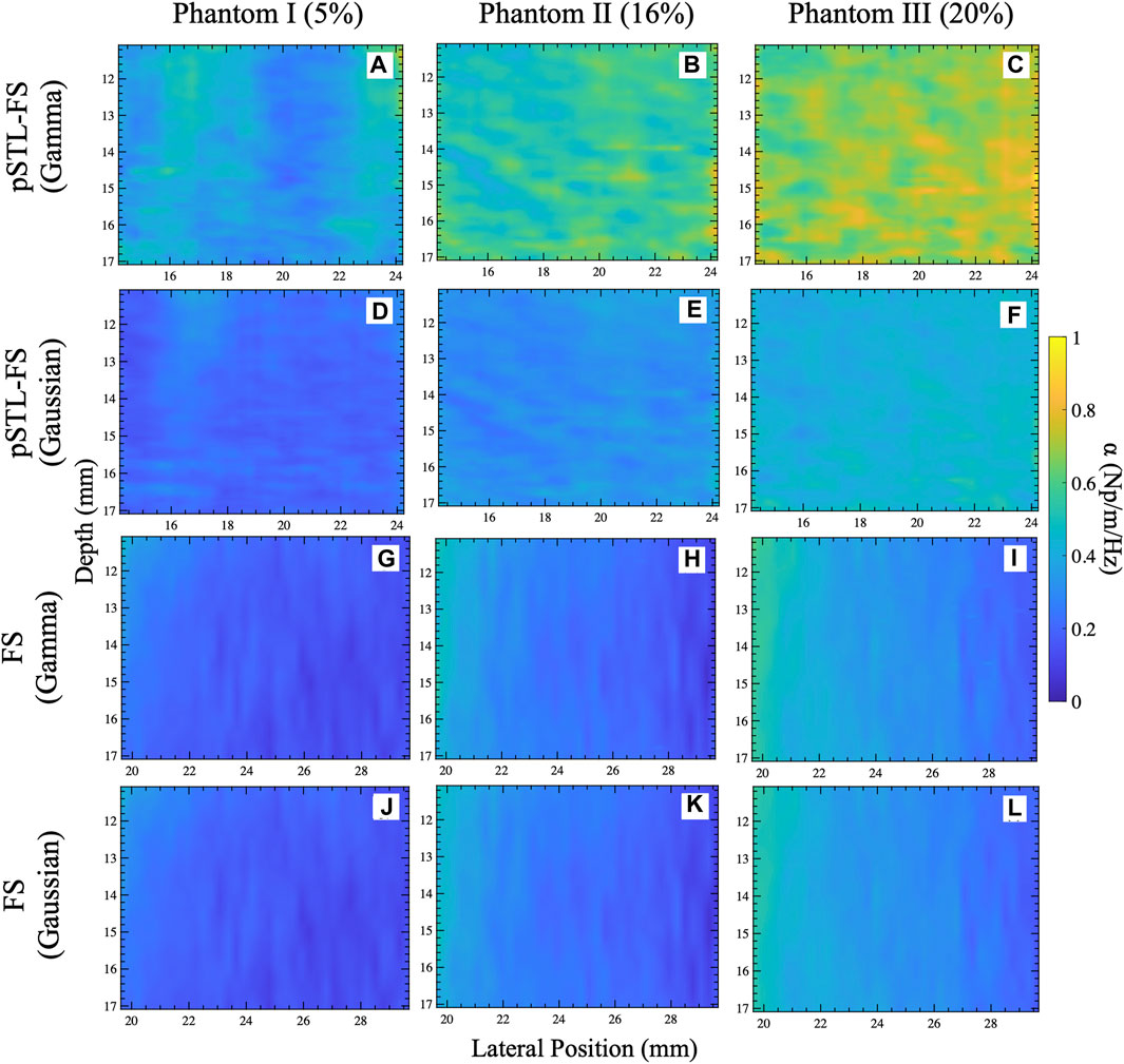
Figure 3. Attenuation coefficient maps obtained for the selected ROI shown in Figure 2E for phantoms I (A,D,G,J), II (B,E,H,K), and III (C,F,I,L). The attenuation coefficient maps were reconstructed using pSTL-FS with Gamma (A–C) and Gaussian (D–F) fitting. In addition, this figure depicts the attenuation coefficient maps reconstructed using the original FS method with a Gamma (C,F,I) and Gaussian (J,K,L) fitting.

Figure 4

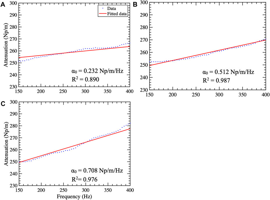
Figure 4. Attenuation curves computed using the AMUSE technique for phantoms I (A), II (B), and III (C). The blue dots and the red line represent the data and the fitted curve, respectively. The attenuation coefficient ${\alpha }_0$ is calculated by fitting the attenuation curve to a linear function. The plots include the attenuation coefficient and the goodness of the fit (R²). The attenuation coefficients varied with the oil percentage, which is consistent with the observations from the pSTL-FS (Gamma) results.

Figure 5

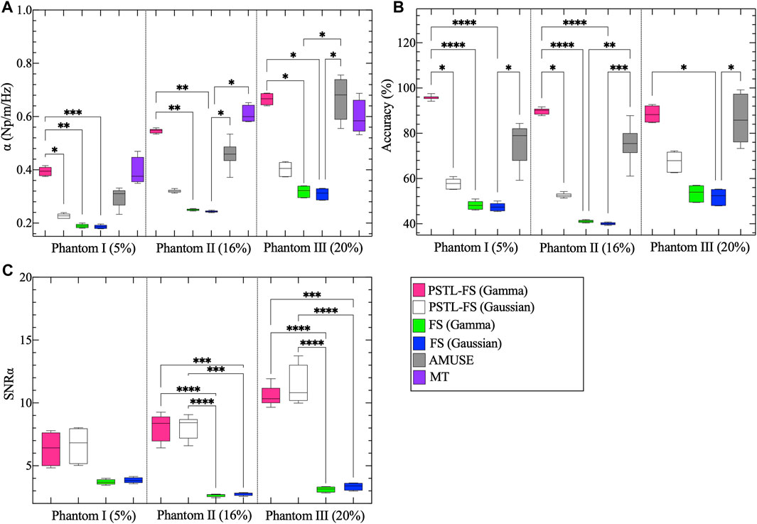
Figure 5. Box plots of the mean attenuation coefficients calculated of the selected ROI shown in Figure 2C for phantoms I, II, and III. (A) Showing the mean attenuation coefficients reconstructed using the pSTL-FS method (Gamma and Gaussian), FS (Gamma and Gaussian), AMUSE, and mechanical testing (MT). Pink, white, green, blue, gray, and purple represent pSTL-FS (Gamma), pSTL-FS (Gaussian), FS (Gamma), FS (Gaussian), AMUSE, and MT, respectively. Also shown are the box plots of the accuracy of the mean attenuation coefficient estimates of phantoms I, II, and III. Accuracy was computed with respect to MT (B). Box plot (C) presents the signal-to-noise ratio (SNR_α) of the attenuation coefficient maps computed using pSTL-FS (Gamma and Gaussian) and FS (Gamma and Gaussian) in phantoms.

Table 1

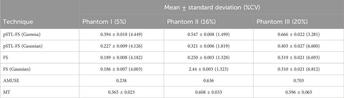
Table 1. Mean, standard deviation and percentage coefficient of variation for attenuation coefficient computed using repeated phantom acquisitions using pSTL-FS (Gamma and Gaussian), FS (Gamma and Gaussian), AMUSE, and MT approaches.

Figure 6 shows representative examples of the shear wave spectra obtained with two identical push beam positions (x₀ and x₁) in all three phantoms. Each spectrum was fitted to Gaussian (Figures 6A, C, E) and Gamma (Figures 6B, D, F) distributions. Fitting the spectrum corresponding to the first push beam to a Gaussian distribution produced a higher R² value compared to when the shear wave spectrum obtained from the second push beam was fitted the Gaussian distribution. Fitting to a Gamma distribution resulted in similar R² value for both pushes, except phantom II.

Figure 6

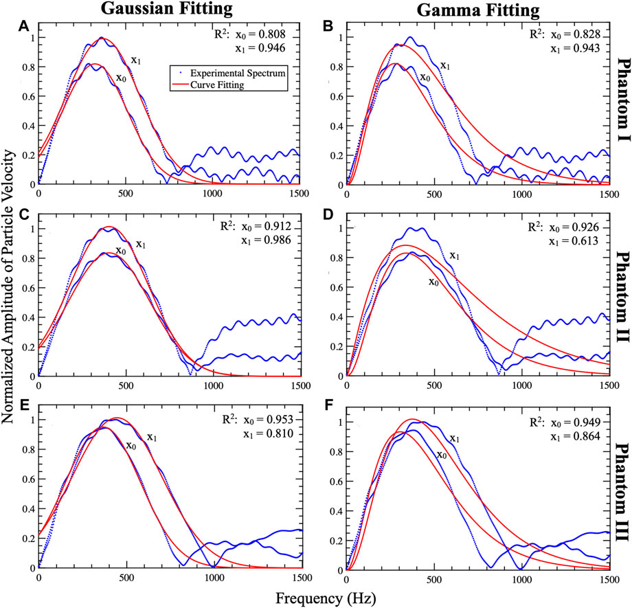
Figure 6. Representative examples of Gaussian and Gamma curve fitting of the shear wave spectrum pair. This plot includes the shear wave profiles (particle velocity profiles) obtained from Phantom I (A,B), II (C,D), and (E,F). The profiles (blue) were fitted to Gaussian (A,C,E) and Gamma (B,D,F) distributions which are shown in red. The shear waves generated from pushes at lateral positions x₁ and x₂ are tracked at x_t. For all phantoms x₀, x₁, x_t, and depth (z) are set to 13.3 mm, 14.5 mm, 18.7 mm, and 16.53 mm, respectively. The plots include R² of the shear wave spectrum pair fits. The Gaussian fit (A,C,E) demonstrated a better fit for x₁ compared to x₂ due to fixing the standard deviation to that of x₁. The Gamma fits (B,D,F) showed less variation between the shear wave spectra pair. By observing the overlap of the profiles and the fits it is noted that the Gaussian fit is more accurate than the Gamma fit.

Supplementary Figure S1 shows representative examples of R² images computed when shear wave spectra were modeled as a Gamma distribution and a Gaussian distribution. In both cases, the resulting R² values exceeded 0.94, indicating that either function (Gaussian or Gamma) was a good model of the shear wave spectra generated in the viscoelastic phantoms employed in this study. The mean and standard deviation of the R² values calculated over the selected ROI (see Figure 2E) of the three phantoms confirmed this observation (Table 2); for both distributions the mean R² values were very high (ranging from 0.959 to 0.964) and low standard deviation (ranging from 0.001 to 0.004) demonstrating their suitability for modeling the shear wave spectra generated in this study.

Table 2

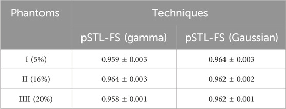
Table 2. Mean and standard deviation of the R² calculated for the shear wave spectra using Gamma and Gaussian curve fits in the phantoms.

In vivo study

Figure 7 shows representative examples of attenuation coefficient maps computed with the pSTL-FS and the standard FS approach using Gamma and Gaussian distributions. Attenuation coefficient images contained regions with higher attenuations when shear wave spectra were assumed to be a Gamma (Figures 7A,B) than Gaussian (Figures 7C,D) distribution during pSTL-FS imaging. The pSTL-FS with a Gamma distribution produced attenuation maps with visibly higher attenuation values in OB mouse than in control mouse (Figures 7A,B). However, as in the phantom studies, assuming a Gaussian distribution resulted in lower attenuation values for both groups. The standard FS, with either Gamma or Gaussian distribution, produced attenuation maps with lower values compared to pSTL-FS (Figures 7E–H). The AMUSE method produced attenuation coefficient values higher in the OB mouse than in the control mouse. (see Supplementary Figure S2). Figure 8 shows the box plot of the mean attenuation coefficients for the grouped control and obese mice computed using pSTL-FS (Gamma and Gaussian), standard FS (Gamma and Gaussian), and AMUSE. pSTL-FS (Gamma) and AMUSE resulted in higher attenuation coefficient values than pSTL-FS (Gaussian) and FS (Gamma and Gaussian) which is consistent with phantom studies. Statistical analysis revealed that pSTL-FS with a Gamma distribution had the highest significant difference between control and obese mice than the other techniques (p-value = < 0.0001) (see Figure 8).

Figure 7

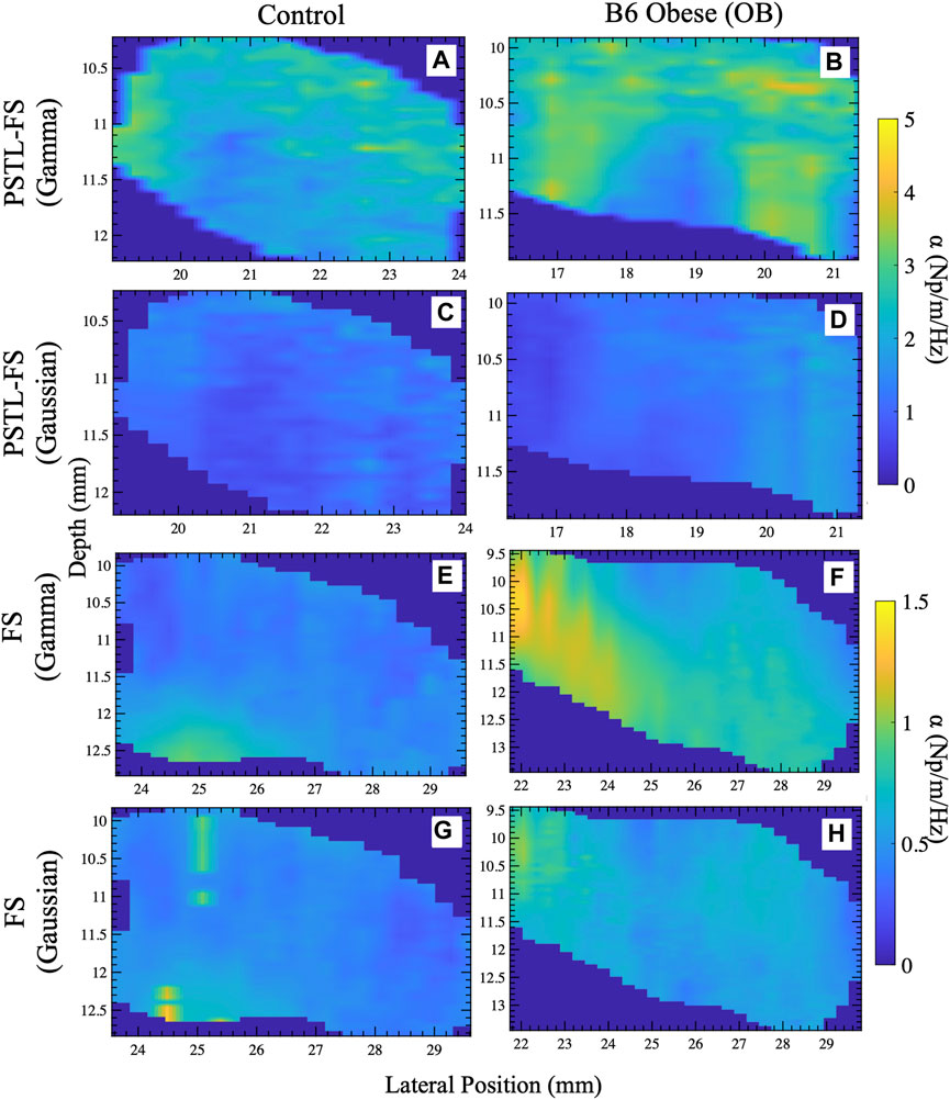
Figure 7. Representative attenuation coefficient maps of the livers reconstructed with different approaches for control and obese mice. Attenuation coefficient maps reconstructed with the pSTL-FS incorporating Gamma (A,B) and Gaussian (C,D) along with the FS technique with Gamma (E,F) and Gaussian (G,H) fitting.

Figure 8

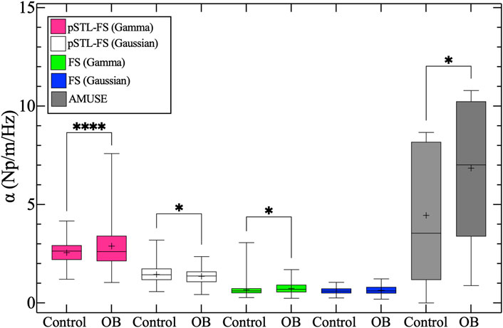
Figure 8. Box plots of the mean attenuation coefficient of the whole liver for control and obese (OB) groups. Pink, white, green, blue, and gray boxes represent the attenuation coefficient estimates for pSTL-FS (Gamma), pSTL-FS (Gaussian), and FS (Gamma), FS (Gaussian), and AMUSE, respectively.

Supplementary Figure S3 shows representative R² images computed for murine liver during pSTL-FS when assuming a Gamma (Supplementary Figures S3A, C) and Gaussian (Supplementary Figures S3B, D) fits. The Gamma fit resulted in better R² maps compared to the Gaussian fit. Overall, the R² maps show spatial variability which is more prominent when using Gaussian fit (Supplementary Figures S3B, D, F, H). The R² mean values for the Gamma fit 0.765–0.807 and standard deviation ranging from 0.058–0.116 while the Gaussian fit ranged from 0.599–0.648 with a standard deviation ranging from 0.0541–0.089.

Supplementary Figure S4 shows the attenuation maps reconstructed with pSTL-FS (Gamma) when using a single push pair (fixing $\left.\Delta P\right)$ versus multiple push pairs (varying $\left.\Delta P\right)$. Using a single push pair, while still varying the tracking location, produced regions with higher attenuation values (Supplementary Figures S4A, C). These regions were also present in the R-square maps (Supplementary Figures S4E, G), with lower R² values. The attenuation maps that utilized multiple push showed smoother maps (Supplementary Figures S4B, D) and the R² maps showed spatially consistent values (Supplementary Figures S4F, H).

Discussion

In this paper, we explored the feasibility of using pSTL-FS to estimate shear wave attenuation and evaluated whether there is a difference in performance when the shear wave spectra are modeled as Gaussian or Gamma distributions. The primary findings of this work were as follows:

1. pSTL-FS yielded more accurate results in phantoms, when shear wave spectra were assumed to be a Gamma distribution vs. a Gaussian distribution (Figure 5B).

2. The mean attenuation coefficients estimated by pSTL-FS/Gamma (84.69%–97.55% accuracy) and AMUSE (59.25%–99.22% accuracy) were comparable, while those estimated by pSTL-FS/gaussian and FS were lower for all phantoms.

3. pSTL-FS is not affected by the proximity and distance from the push beam. pSTL-FS reduced the artifacts of higher attenuation values closer to the push beam and of lower attenuation values farther from the push beam (see Figure 3).

4. The Gaussian fitting yielded similar R² values compared to Gamma fitting in phantoms (Figure 6, Supplementary Figures S1, S3).

5. The attenuation coefficient maps of the livers show spatial variability, with pSTL-FS/Gamma having higher estimates than pSTL-FS/Gaussian and FS (Gamma and Gaussian) (Figure 7). The FS approach to attenuation maps with lower values compared to pSTL-FS and AMUSE (Figure 7).

6. The attenuation coefficient estimates from pSTL-FS (Gamma) had the highest significant difference between control and obese mice than pSTL-FS (Gaussian), FS (Gamma and Gaussian), and AMUSE (p-value <0.0001).

Figure 3 demonstrates that the attenuation coefficient maps reconstructed with pSTL-FS (Gamma) show spatial heterogeneity in the homogeneous phantoms. An issue could be the process used to fabricate the viscoelastic phantoms. Although the mixture was stirred to ensure uniform oil distribution throughout the phantom, some separation is expected. Consequently, we plan to improve our manufacturing process to overcome this problem. Researchers have reported spatially varying attenuation maps consistent with those produced by FS (Figures 3G–I) [30–32]. Their approaches used a sliding window approach resulting in excessively smoother maps in phantom and duck livers [30–32].

One of the challenges in quantifying attenuation is the rapid shear wave dissipation in the medium as they propagate further from the push beam [26]. This was clearly visible in the attenuation maps reconstructed using the FS method (see Figures 3G–L), as the attenuation maps showed a gradual decrease in the attenuation values moving from right to left. Although the FS method is independent of geometric spreading, the shear wave amplitude will dissipate as the shear wave propagates, reducing the signal-to-noise ratio and leading to inaccurate attenuation estimates. This is not the case with pSTL-FS approach because the tracking is performed a single location further from the push beam. The attenuation maps reconstructed with pSTL-FS showed no gradual changes in attenuation (see Figures 3A–F).

Researchers have argued that the shear wave generated by the acoustic radiation force pulse should be represented by a Gaussian fit [33,34]. In contrast, other researchers have chosen the Gamma distribution as a more accurate fit for the shear wave spectrum [30–32]. In this work, we demonstrated that fitting the shear wave spectra to Gamma and Gaussian distributions resulted in similar R² values (Figure 6), indicating both distributions are a good fit for shear wave spectra. However, the attenuation coefficient values were drastically different with Gamma distribution producing more accurate results for all phantoms (see Figure 5; Supplementary Figures S1, S3). This suggests that a Gamma distribution is a better fit when estimating the attenuation coefficient using the FS approach.

Studies have shown that fat deposition in the liver is reflected in viscosity [52], and one would expected the attenuation coefficient to be higher in obese mice. Figure 8 shows that pSTL-FS (Gamma) and the AMUSE method result in higher variation in the attenuation coefficient values for the obese group which is reflected by the whiskers and interquartile range of the latter techniques. However, AMUSE method had greater interquartile range between the two group and a less significant difference between groups compared to pSTL-FS (Gamma). There is a significant difference in the attenuation estimates produced by pSTL-FS (Gaussian) between control and obese groups, however the control had higher attenuation values that the obese. For the FS (Gamma), control group had a higher attenuation coefficient range however, the interquartile range was higher in the obese group (Figure 8). This would suggest some artifacts or outliers in the control group.

Researchers reported that in vivo SWE application is hindered by noise and motion artifacts [28,53–55]. Performing repeated acquisitions and averaging the measurement is a common practice used to overcome these challenges. Nonetheless, researchers have shown that the properties of the shear wave are heavily dependent on the medium, and a corrupt push beam may be caused due tissue heterogeneity [56]. Therefore, relying on a repeated push beam located at a single lateral position might not reduce error. The laterally shifting push beams overcome this challenge and this was clearly shown when comparing the attenuation maps reconstructed with a single push vs. multiple pushes (see Supplementary Figure S4). Using a single push pair resulted in line artifacts which was not the case when using multiple pushes (see Supplementary Figure S4).

A limitation of pSTL-FS is the significant computational time required to reconstruct attenuation coefficient maps, as detailed in Table 3. Attenuation maps generated using pSTL-FS with Gamma and Gaussian fitting take approximately 5.26 ± 2.17 h and 1.14 ± 0.37 h, respectively. In comparison, the FS method, with an equivalent number of pushes, takes about 10.81 ± 3.94 h and 7.22 ± 1.78 h for Gamma and Gaussian distributions, respectively. Despite both pSTL-FS and FS utilizing an equivalent number of pushes, the FS approach demands roughly twice the computational time required by pSTL-FS. This increased time could be attributed to the window-based approach employed in the FS method. Moreover, Gaussian fitting is expected to be quicker in generating an attenuation map since this approach solves for only two parameters (centroid frequency and amplitude), given that the standard deviation for the shear wave spectra is fixed. To overcome this challenge, GPU processing can generate the attenuation maps parallelly. Another limitation of this study is that we did not characterize the livers' viscoelastic properties using another method, such as atomic force microscopy, nor did we evaluate how changing oil concentrations impact shear wave attenuation measurements. Researchers have demonstrated that the speed of sound remains relatively constant for different oil concentrations [57]. However, it's uncertain if the oil concentration used in their research is similar to our study. Therefore, we intend to conduct further research to examine whether sound speed is consistent throughout the range of oil concentrations used in our study. In future work, we aim to use atomic force microscopy to measure complex shear modulus to derive the attenuation coefficient. In addition, when calculating the attenuation coefficient, we assumed that it is linearly dependent on frequency. Researchers have reported that some biological tissues exhibit nonlinear behavior, especially at higher frequencies (1,000 Hz) [58–60].

Table 3

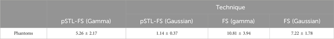
Table 3. Processing time (hours) needed to reconstruct an attenuation map for an area of 200 mm² using PSTL-FS and FS in phantoms.

Conclusion

In this study, we extended the pSTL-SWE technique to reconstruct attenuation coefficient maps by incorporating the FS approach. This technique synthesizes multiple datasets by using multiple laterally-shifted pushes followed by plane wave tracking, used to reduce the effect of noise and speckle bias. Averaging of the attenuation maps produces a single attenuation map with higher accuracy and ${SNR}_{\alpha }$ compared to the FS approach. Assuming a Gamma distribution led to higher accuracies than assuming a Gaussian distribution. The results of in vivo imaging favor the use of pSTL-FS over FS and AMUSE for heterogeneous biological tissues.

Data availability statement

The raw data supporting the conclusion of this article will be made available by the authors, without undue reservation.

Ethics statement

The animal study was approved by the University of Rochester Committee on Animal Resources. The study was conducted in accordance with the local legislation and institutional requirements.

Author contributions

RM: Data curation, Formal Analysis, Investigation, Methodology, Writing–original draft. KI: Investigation, Writing–review and editing. SG: Funding acquisition, Supervision, Writing–review and editing. MD: Funding acquisition, Supervision, Writing–review and editing, Conceptualization, Project administration, Resources.

Funding

The author(s) declare financial support was received for the research, authorship, and/or publication of this article. This work was supported by NIH Grants R01EB032337, R01CA236390, and R01CA230277.

Conflict of interest

The authors declare that the research was conducted in the absence of any commercial or financial relationships that could be construed as a potential conflict of interest.

Publisher’s note

All claims expressed in this article are solely those of the authors and do not necessarily represent those of their affiliated organizations, or those of the publisher, the editors and the reviewers. Any product that may be evaluated in this article, or claim that may be made by its manufacturer, is not guaranteed or endorsed by the publisher.

Supplementary material

The Supplementary Material for this article can be found online at: https://www.frontiersin.org/articles/10.3389/fphy.2024.1326770/full#supplementary-material

Abbreviations

AMUSE, Attenuation measuring ultrasound elastography; FS, Frequency Shift; KVFD, Kelvin-Voigt fractional derivative model; SWA, Shear wave attenuation; PDF, probability density function; pSTL-FS, plane wave single-track location-based frequency shift; pSTL-SWE, plane wave single-track location shear wave elastography; SWE, Shear wave elastography; SWS, Shear wave speed.

References

1. Mierke CT. The fundamental role of mechanical properties in the progression of cancer disease and inflammation. Rep Prog Phys (2014) 77:076602. doi:10.1088/0034-4885/77/7/076602

PubMed Abstract | CrossRef Full Text | Google Scholar

2. Handorf AM, Zhou Y, Halanski MA, Li W-J. Tissue stiffness dictates development, homeostasis, and disease progression. Organogenesis (2015) 11:1–15. doi:10.1080/15476278.2015.1019687

PubMed Abstract | CrossRef Full Text | Google Scholar

3. Butcher DT, Alliston T, Weaver VM. A tense situation: forcing tumour progression. Nat Rev Cancer (2009) 9:108–22. doi:10.1038/nrc2544

PubMed Abstract | CrossRef Full Text | Google Scholar

4. Sarvazyan AP, Rudenko OV, Swanson SD, Fowlkes JB, Emelianov SY. Shear wave elasticity imaging: a new ultrasonic technology of medical diagnostics. Ultrasound Med Biol (1998) 24:1419–35. doi:10.1016/s0301-5629(98)00110-0

PubMed Abstract | CrossRef Full Text | Google Scholar

5. Castera L, Forns X, Alberti A. Non-invasive evaluation of liver fibrosis using transient elastography. J Hepatol (2008) 48:835–47. doi:10.1016/j.jhep.2008.02.008

PubMed Abstract | CrossRef Full Text | Google Scholar

6. Chang JM, Moon WK, Cho N, Yi A, Koo HR, Han W, et al. Clinical application of shear wave elastography (SWE) in the diagnosis of benign and malignant breast diseases. Breast Cancer Res Treat (2011) 129:89–97. doi:10.1007/s10549-011-1627-7

PubMed Abstract | CrossRef Full Text | Google Scholar

7. Kelly P. Solid mechanics part I: an introduction to solid mechanics. A Creat Commons Attributions, Mountain View, CA (2013):94042.

Google Scholar

8. Roylance D Engineering viscoelasticity. Cambridge MA: Department of Materials Science and Engineering–Massachusetts Institute of Technology (2001). p. 1–37. 2139.

Google Scholar

9. Streitberger K-J, Sack I, Krefting D, Pfüller C, Braun J, Paul F, et al. Brain viscoelasticity alteration in chronic-progressive multiple sclerosis. PloS one (2012) 7:e29888. doi:10.1371/journal.pone.0029888

PubMed Abstract | CrossRef Full Text | Google Scholar

10. Barry CT, Mills B, Hah Z, Mooney RA, Ryan CK, Rubens DJ, et al. Shear wave dispersion measures liver steatosis. Ultrasound Med Biol (2012) 38:175–82. doi:10.1016/j.ultrasmedbio.2011.10.019

PubMed Abstract | CrossRef Full Text | Google Scholar

11. Ormachea J, Parker KJ. Comprehensive viscoelastic characterization of tissues and the inter-relationship of shear wave (group and phase) velocity, attenuation and dispersion. Ultrasound Med Biol (2020) 46:3448–59. doi:10.1016/j.ultrasmedbio.2020.08.023

PubMed Abstract | CrossRef Full Text | Google Scholar

12. Garcovich M, Paratore M, Ainora ME, Riccardi L, Pompili M, Gasbarrini A, et al. Shear wave dispersion in chronic liver disease: from physical principles to clinical usefulness. J Personalized Med (2023) 13:945. doi:10.3390/jpm13060945

CrossRef Full Text | Google Scholar

13. Furuichi Y, Sugimoto K, Oshiro H, Abe M, Takeuchi H, Yoshimasu Y, et al. Elucidation of spleen elasticity and viscosity in a carbon tetrachloride rat model of liver cirrhosis using a new ultrasound elastography. J Med Ultrason (2021) 48:431–7. doi:10.1007/s10396-021-01110-5

CrossRef Full Text | Google Scholar

14. Parker K, Szabo T, Holm S. Towards a consensus on rheological models for elastography in soft tissues. Phys Med Biol (2019) 64:215012. doi:10.1088/1361-6560/ab453d

PubMed Abstract | CrossRef Full Text | Google Scholar

15. Chen S, Fatemi M, Greenleaf JF. Quantifying elasticity and viscosity from measurement of shear wave speed dispersion. The J Acoust Soc America (2004) 115:2781–5. doi:10.1121/1.1739480

PubMed Abstract | CrossRef Full Text | Google Scholar

16. Taylor LS, Lerner AL, Rubens DJ, Parker KJ. A Kelvin-Voight fractional derivative model for viscoelastic characterization of liver tissue. ASME Int Mech Eng Congress Exposition (2002) 447–8. doi:10.1115/IMECE2002-3260

CrossRef Full Text | Google Scholar

17. Hossain MM, Gallippi CM. Viscoelastic response ultrasound derived relative elasticity and relative viscosity reflect true elasticity and viscosity: in silico and experimental demonstration. IEEE Trans Ultrason ferroelectrics, frequency Control (2019) 67:1102–17. doi:10.1109/tuffc.2019.2962789

CrossRef Full Text | Google Scholar

18. Vappou J, Maleke C, Konofagou EE. Quantitative viscoelastic parameters measured by harmonic motion imaging. Phys Med Biol (2009) 54:3579–94. doi:10.1088/0031-9155/54/11/020

PubMed Abstract | CrossRef Full Text | Google Scholar

19. Rouze NC, Deng Y, Trutna CA, Palmeri ML, Nightingale KR. Characterization of viscoelastic materials using group shear wave speeds. IEEE Trans Ultrason ferroelectrics, frequency Control (2018) 65:780–94. doi:10.1109/tuffc.2018.2815505

CrossRef Full Text | Google Scholar

20. Hossain MM, Konofagou EE. Feasibility of phase velocity imaging using multi frequency oscillation-shear wave elastography. IEEE Trans Biomed Eng (2023) 71:607–20. doi:10.1109/tbme.2023.3309996

CrossRef Full Text | Google Scholar

21. Amador C, Urban MW, Chen S, Greenleaf JF. Loss tangent and complex modulus estimated by acoustic radiation force creep and shear wave dispersion. Phys Med Biol (2012) 57:1263–82. doi:10.1088/0031-9155/57/5/1263

PubMed Abstract | CrossRef Full Text | Google Scholar

22. Viola F, Walker WF. Radiation force imaging of viscoelastic properties with reduced artifacts. IEEE Trans Ultrason ferroelectrics, frequency Control (2003) 50:736–42. doi:10.1109/tuffc.2003.1209564

PubMed Abstract | CrossRef Full Text | Google Scholar

23. Kijanka P, Urban MW. Local phase velocity based imaging of viscoelastic phantoms and tissues. IEEE Trans Ultrason ferroelectrics, frequency Control (2020) 68:389–405. doi:10.1109/tuffc.2020.2968147

PubMed Abstract | CrossRef Full Text | Google Scholar

24. Kazemirad S, Bernard S, Hybois S, Tang A, Cloutier G. Ultrasound shear wave viscoelastography: model-independent quantification of the complex shear modulus. IEEE Trans Ultrason ferroelectrics, frequency Control (2016) 63:1399–408. doi:10.1109/tuffc.2016.2583785

CrossRef Full Text | Google Scholar

25. Budelli E, Brum J, Bernal M, Deffieux T, Tanter M, Lema P, et al. A diffraction correction for storage and loss moduli imaging using radiation force based elastography. Phys Med Biol (2016) 62:91–106. doi:10.1088/1361-6560/62/1/91

PubMed Abstract | CrossRef Full Text | Google Scholar

26. Parker KJ, Ormachea J, Will S, Hah Z. Analysis of transient shear wave in lossy media. Ultrasound Med Biol (2018) 44:1504–15. doi:10.1016/j.ultrasmedbio.2018.03.014

PubMed Abstract | CrossRef Full Text | Google Scholar

27. Nenadic I, Urban MW, Qiang B, Chen S, Greenleaf J. Model-free quantification of shear wave velocity and attenuation in tissues and its in vivo application. J Acoust Soc America (2013) 134:4011. doi:10.1121/1.4830632

CrossRef Full Text | Google Scholar

28. Nightingale KR, Rouze NC, Rosenzweig SJ, Wang MH, Abdelmalek MF, Guy CD, et al. Derivation and analysis of viscoelastic properties in human liver: impact of frequency on fibrosis and steatosis staging. IEEE Trans Ultrason ferroelectrics, frequency Control (2015) 62:165–75. doi:10.1109/tuffc.2014.006653

PubMed Abstract | CrossRef Full Text | Google Scholar

29. Quan Y, Harris JM. Seismic attenuation tomography using the frequency shift method. Geophysics (1997) 62:895–905. doi:10.1190/1.1444197

CrossRef Full Text | Google Scholar

30. Bernard S, Kazemirad S, Cloutier G. A frequency-shift method to measure shear-wave attenuation in soft tissues. IEEE Trans Ultrason ferroelectrics, frequency Control (2016) 64:514–24. doi:10.1109/tuffc.2016.2634329

CrossRef Full Text | Google Scholar

31. Yazdani L, Bhatt M, Rafati I, Tang A, Cloutier G. The revisited frequency-shift method for shear wave attenuation computation and imaging. IEEE Trans Ultrason Ferroelectrics, Frequency Control (2022) 69:2061–74. doi:10.1109/tuffc.2022.3166448

CrossRef Full Text | Google Scholar

32. Kijanka P, Urban MW. Two-point frequency shift method for shear wave attenuation measurement. IEEE Trans Ultrason ferroelectrics, frequency Control (2019) 67:483–96. doi:10.1109/tuffc.2019.2945620

CrossRef Full Text | Google Scholar

33. Parker KJ, Baddour N. The Gaussian shear wave in a dispersive medium. Ultrasound Med Biol (2014) 40:675–84. doi:10.1016/j.ultrasmedbio.2013.10.023

PubMed Abstract | CrossRef Full Text | Google Scholar

34. Rouze NC, Palmeri ML, Nightingale KR. An analytic, Fourier domain description of shear wave propagation in a viscoelastic medium using asymmetric Gaussian sources. J Acoust Soc America (2015) 138:1012–22. doi:10.1121/1.4927492

PubMed Abstract | CrossRef Full Text | Google Scholar

35. Ahmed R, Gerber SA, Mcaleavey SA, Schifitto G, Doyley MM. Plane-wave imaging improves single-track location shear wave elasticity imaging. IEEE Trans Ultrason ferroelectrics, frequency Control (2018) 65:1402–14. doi:10.1109/tuffc.2018.2842468

CrossRef Full Text | Google Scholar

36. Elegbe EC, Mcaleavey SA. Single tracking location methods suppress speckle noise in shear wave velocity estimation. Ultrason Imaging (2013) 35:109–25. doi:10.1177/0161734612474159

PubMed Abstract | CrossRef Full Text | Google Scholar

37. Loupas T, Powers J, Gill RW. An axial velocity estimator for ultrasound blood flow imaging, based on a full evaluation of the Doppler equation by means of a two-dimensional autocorrelation approach. IEEE Trans Ultrason ferroelectrics, frequency Control (1995) 42:672–88. doi:10.1109/58.393110

CrossRef Full Text | Google Scholar

38. Ahmed R, Ye J, Gerber SA, Linehan DC, Doyley MM. Preclinical imaging using single track location shear wave elastography: monitoring the progression of murine pancreatic tumor liver metastasis in vivo. IEEE Trans Med Imaging (2020) 39:2426–39. doi:10.1109/tmi.2020.2971422

PubMed Abstract | CrossRef Full Text | Google Scholar

39. Nenadic IZ, Qiang B, Urban MW, Zhao H, Sanchez W, Greenleaf JF, et al. Attenuation measuring ultrasound shearwave elastography and in vivo application in post-transplant liver patients. Phys Med Biol (2016) 62:484–500. doi:10.1088/1361-6560/aa4f6f

PubMed Abstract | CrossRef Full Text | Google Scholar

40. Poul SS, Ormachea J, Gary RG, Parker KJ. Comprehensive experimental assessments of rheological models’ performance in elastography of soft tissues. Acta Biomater (2022) 146:259–73. doi:10.1016/j.actbio.2022.04.047

PubMed Abstract | CrossRef Full Text | Google Scholar

41. Zhang M, Castaneda B, Wu Z, Nigwekar P, Joseph JV, Rubens DJ, et al. Congruence of imaging estimators and mechanical measurements of viscoelastic properties of soft tissues. Ultrasound Med Biol (2007) 33:1617–31. doi:10.1016/j.ultrasmedbio.2007.04.012

PubMed Abstract | CrossRef Full Text | Google Scholar

42. Carstensen EL, Parker KJ. Physical Models of Tissue in Shear Fields11This article is dedicated to our friend and colleague, Robert C. Waag. Ultrasound Med Biol (2014) 40:655–74. doi:10.1016/j.ultrasmedbio.2013.11.001

PubMed Abstract | CrossRef Full Text | Google Scholar

43. Oler AT, Attie AD. A rapid, microplate SNP genotype assay for the leptin allele. J lipid Res (2008) 49:1126–9. doi:10.1194/jlr.d800002-jlr200

PubMed Abstract | CrossRef Full Text | Google Scholar

44. Sanna V, Di Giacomo A, La Cava A, Lechler RI, Fontana S, Zappacosta S, et al. Leptin surge precedes onset of autoimmune encephalomyelitis and correlates with development of pathogenic T cell responses. J Clin Invest (2003) 111:241–50. doi:10.1172/jci16721

PubMed Abstract | CrossRef Full Text | Google Scholar

45. Mancuso P, Gottschalk A, Phare SM, Peters-Golden M, Lukacs NW, Huffnagle GB. Leptin-deficient mice exhibit impaired host defense in Gram-negative pneumonia. J Immunol (2002) 168:4018–24. doi:10.4049/jimmunol.168.8.4018

PubMed Abstract | CrossRef Full Text | Google Scholar

46. Siegmund B, Lehr HA, Fantuzzi G. Leptin: a pivotal mediator of intestinal inflammation in mice. Gastroenterology (2002) 122:2011–25. doi:10.1053/gast.2002.33631

PubMed Abstract | CrossRef Full Text | Google Scholar

47. Malik N, Carter ND, Murray JF, Scaramuzzi R, Wilson C, Stock M. Leptin requirement for conception, implantation, and gestation in the mouse. Endocrinology (2001) 142:5198–202. doi:10.1210/endo.142.12.8535

PubMed Abstract | CrossRef Full Text | Google Scholar

48. Fantuzzi G, Faggioni R. Leptin in the regulation of immunity, inflammation, and hematopoiesis. J Leukoc Biol (2000) 68:437–46. doi:10.1189/jlb.68.4.437

PubMed Abstract | CrossRef Full Text | Google Scholar

49. Ewart-Toland A, Mounzih K, Qiu J, Chehab FF. Effect of the genetic background on the reproduction of leptin-deficient obese mice. Endocrinology (1999) 140:732–8. doi:10.1210/endo.140.2.6470

PubMed Abstract | CrossRef Full Text | Google Scholar

50. Zhang Y, Proenca R, Maffei M, Barone M, Leopold L, Friedman JM. Positional cloning of the mouse obese gene and its human homologue. Nature (1994) 372:425–32. doi:10.1038/372425a0

PubMed Abstract | CrossRef Full Text | Google Scholar

51. Coleman D, Hummel K. The influence of genetic background on the expression of the obese (Ob) gene in the mouse. Diabetologia (1973) 9:287–93. doi:10.1007/bf01221856

PubMed Abstract | CrossRef Full Text | Google Scholar

52. Parker K, Ormachea J, Drage M, Kim H, Hah Z. The biomechanics of simple steatosis and steatohepatitis. Phys Med Biol (2018) 63:105013. doi:10.1088/1361-6560/aac09a

PubMed Abstract | CrossRef Full Text | Google Scholar

53. Fatemi M, Gregory A, Bayat M, Denis M, Alizad A. Challenges in estimation of tissue elasticity using low-frequency shear waves. In: 22nd International Congress on Sound and Vibration, ICSV 2015, 2015. International Institute of Acoustics and Vibrations; 12-16 July 2015; Florence, Italy (2015).

Google Scholar

54. Nightingale K, Mcaleavey S, Trahey G. Shear-wave generation using acoustic radiation force: in vivo and ex vivo results. Ultrasound Med Biol (2003) 29:1715–23. doi:10.1016/j.ultrasmedbio.2003.08.008

PubMed Abstract | CrossRef Full Text | Google Scholar

55. Palmeri ML, Wang MH, Rouze NC, Abdelmalek MF, Guy CD, Moser B, et al. Noninvasive evaluation of hepatic fibrosis using acoustic radiation force-based shear stiffness in patients with nonalcoholic fatty liver disease. J Hepatol (2011) 55:666–72. doi:10.1016/j.jhep.2010.12.019

PubMed Abstract | CrossRef Full Text | Google Scholar

56. Kumar V, Denis M, Gregory A, Bayat M, Mehrmohammadi M, Fazzio R, et al. Viscoelastic parameters as discriminators of breast masses: initial human study results. PloS one (2018) 13:e0205717. doi:10.1371/journal.pone.0205717

PubMed Abstract | CrossRef Full Text | Google Scholar

57. Sjöstrand S, Meirza B, Grassi L, Svensson I, Camargo LC, Pavan TZ, et al. Tuning viscoelasticity with minor changes in speed of sound in an ultrasound phantom material. Ultrasound Med Biol (2020) 46:2070–8. doi:10.1016/j.ultrasmedbio.2020.03.028

PubMed Abstract | CrossRef Full Text | Google Scholar

58. Szabo TL. Time domain wave equations for lossy media obeying a frequency power law. J Acoust Soc America (1994) 96:491–500. doi:10.1121/1.410434

CrossRef Full Text | Google Scholar

59. Ophir J, Shawker T, Maklad N, Miller J, Flax S, Narayana P, et al. Attenuation estimation in reflection: progress and prospects. Ultrason Imaging (1984) 6:349–95. doi:10.1177/016173468400600401

PubMed Abstract | CrossRef Full Text | Google Scholar

60. Narayana PA, Ophir J. On the frequency dependence of attenuation in normal and fatty liver. IEEE Trans sonics Ultrason (1983) 30:379–82. doi:10.1109/t-su.1983.31444

CrossRef Full Text | Google Scholar