Spatial heterogeneity of long-range dependence and self-similarity of global sea surface chlorophyll concentration with their environmental impact factors analysis

1 Introduction

Phytoplankton serves as the fundamental source of primary production in the world’s oceans. Sea surface chlorophyll concentration (SSCC) is commonly considered as the indicator of the phytoplankton biomass, and was used for primary production estimation [1–3]. It makes a certain contribution to the particulate organic carbon in water and organic matter in sea fog aerosols [4,5]. Studies have shown that phytoplankton, with the highest carbon sequestration capacity in marine ecosystems, can capture 360 billion tons of CO₂ annually, of which 1.39% of CO₂ will be transported to the seabed and stored long-term through the biological pump [6,7]. Understanding the spatial and temporal variation characteristics of SSCC can help estimate the amount of carbon captured in the sea area, clarify the mechanism of marine carbon cycling, and provide scientific bases for algal bloom warning and ocean management.

Based on the autocorrelation characteristics of SSCC, previous studies have developed various time series prediction models, such as long short-term memory neural networks, spatiotemporal attention networks, and hierarchical attention networks [8–10]. When the autocorrelation of SSCC is very strong, it can be considered as long-range dependence. The Hurst exponent is generally used to quantitatively describe the degree of long-range dependence. The generalized fractional Gaussian noise model, generalized Cauchy model, and covariance and variance functions were normally used to calculate the global Hurst exponent [11–13]. Regarding SSCC, the generalized Cauchy model has been utilized to describe the long-range dependence of SSCC at limited number of spatial locations, as well as the self-similarity [14,15]. Although the long-range dependence and self-similarity of SSCC, respectively, show strong and weak characteristics in the above two literatures, it is essential to explore other locations in the oceans for a more comprehensive deduction. A global-scale investigation of the spatial pattern of these two features (i.e., long-range dependence and self-similarity) will not only provide insights into the spatiotemporal variability of SSCC across a broader area but also offer a mathematical perspective to inform ocean management and ecology. Therefore, such an inquiry would lay a solid foundation for the scientific understanding of SSCC, ultimately aiding in the sustainable management of ocean resources.

Remote sensing technology has been a popular tool to monitoring the SSCC variation in large space-time domain. However, the remote sensing data may have some degrees of data missing, so it becomes an important scientific issue to scientifically analyze and accurately interpolate the data using limited data as much as possible. Previous studies have tested five methods, containing of nearest neighbor, bilinear, smooth filter, sharpening filter, and unsharp masking, for interpolation purposes, and the results indicated that these methods had good interpolation accuracy for high-resolution remote sensing images [16]. However, as early as 1994, Rossi et al. [17] pointed out that nearest neighbor or bilinear interpolation cannot fully utilize the spatial information contained in remote sensing data, and indicated that the Kriging method can overcome this deficiency and applied the indicator Kriging in land classification. Considering the advantages of geostatistical methods in interpolation, the family of Kriging and inverse distance weighting method were compared for water quality evaluation, and the results showed that Kriging outperform IDW [18,19]. Although the spatiotemporal Kriging technology has been developed to include temporal information for spatiotemporal interpolation purposes and more accurate prediction will be achieved than the standard Kriging, it still cannot deal with the non-Gaussian distributed or uncertain data with including high order moments [20–23]. The Bayesian maximum entropy method (BME) is currently the most complete and capable interpolation method in the field of spatiotemporal geostatistics by borrowing the strength from the Bayes theory and maximum entropy theory, and it has been widely used in the fields of environmental science, remote sensing, marine science, public health, etc. [24–29]. Although the BME has been employed to assimilate the information from auxiliary variable and machine learning evaluation for improving the spatiotemporal coverage, accuracy and reducing the uncertainty of remote sensing SSCC product [15,30], there is still a lack of direct application of this method to the interpolation of SSCC over a wider range.

SSCC has a direct or indirect response relationship with environmental factors such as sea surface salinity, temperature, wind speed, etc. [31,32]. Specifically, the high correlation between sea surface salinity and nutrient concentration leads to a certain association between the spatial distribution of SSCC and the salinity front [33,34]. A positive correlation between SSCC and sea surface wind speed was found in the east coastal area of Vietnam [35]. Sea surface wind can also affect the vertical stratification and turbulent mixing of seawater by changing the sea surface temperature, and bring nutrients from the bottom of the sea to the sea surface, such as the Ekman suction effect caused by vortex phenomena, which in turn affects the changes and distribution of sea surface chlorophyll [36,37]. Sea surface temperature exhibits close relationship with SSCC, however, the effects of temperature on SSCC may vary at various regions of ocean [15,28,38]. Therefore, it is worthy to explore the environmental impacts on SSCC in a local scale way.

In view of the above considerations, the main objectives of the current study are threefold: to assess the performance of BME in SSCC interpolation, to quantify the long-range dependence and self-similarity of SSCC at a global scale, and to determine the significance of various environmental factors on the SSCC variation.

2 Materials and methods

2.1 Remote sensing data

The remote sensing SSCC data used in this study was obtained from the European Space Agency (ESA) during the period from 29 July 1998 to 31 December2020. The data is a fusion product based on multiple sensors, including Sea-Viewing Wide Field of View Sensor (SeaWiFS), Medium Resolution Imaging Spectrometer (MERIS), Aqua-Moderate Resolution Imaging Spectroradiometer (MODIS), Visible and Infrared Imager/Radiometer Suite (VIIRS), and Ocean and Land Color Instrument (OLCI), with a spatial resolution of 4 km and a temporal resolution of 1 day. To ensure consistency and facilitate analysis with other environmental factors, the original SSCC data was resampled to a product with a spatial resolution of 1° by averaging the SSCC values within each 1-degree grid.

In addition, four environmental factors, including sea surface height anomaly, sea surface salinity, sea surface temperature and wind speed, were regarded as SSCC-related variables. Among them, sea surface height anomaly data was downloaded from Copernicus marine service website, and its spatial and temporal resolution is 0.25° and 1 day, respectively; salinity data were also achieved from Copernicus marine service website, and the spatial and temporal resolutions are 0.25° and 1 week; daily sea surface temperature data were obtained from NOAA optimal interpolated SST with spatial and temporal resolutions of 0.25° and 1 day; wind speed data were achieved by the NOAA NCEI blended Seawinds (NBS v2) with spatial and temporal resolutions of 0.25° and 1 day. The sea surface temperature and wind speed data were resampled to the same resolutions of salinity data.

2.2 Bayesian maximum entropy modeling and spatiotemporal SSCC interpolation

In order to improve the spatiotemporal coverage of remote sensing SSCC data, the BME theory of geostatistics was introduced to absorb the spatiotemporal distribution pattern of SSCC for interpolation purposes. Generally, the spatiotemporal random field (STRF), X(p), was used to describe the spatiotemporal variation of SSCC, where p = (s, t) represents the space-time location, while s = (s₁, s₂) depict the geographical coordinates. To perform spatiotemporal SSCC interpolation, BME absorbs two kinds of knowledge bases (KBs): (a) core or general (G) KB that capturing the space-time SSCC mean trend function $m_X\left(\mathit{p}\right)=\overline{X\left(\mathit{p}\right)}$, and the space-time covariance function $c_X\left(\mathit{p},{\mathit{p}}^{\prime }\right)=\overline{\left[X\left(\mathit{p}\right)-m_X\left(\mathit{p}\right)\right]\left[X\left({\mathit{p}}^{\prime }\right)-m_X\left({\mathit{p}}^{\prime }\right)\right]}$; and (b) site-specific (S) KB including remote sensing SSCC data in the current study. Given both G- and S-KBs into consideration, the probability density functions (PDF) of the possible SSCC values at unmonitored space-time point ${\mathit{p}}_k$ can be calculated by Eq. (1):

$f_K\left({\chi }_k\right)=A^{-1}\int d{\mathit{\chi }}_h{f}_G\left({\mathit{\chi }}_h\right)(1)$

Where ${\mathit{\chi }}_h$ and ${\mathit{\chi }}_k$ denote the SSCC values at point ${\mathit{p}}_h$ and ${\mathit{p}}_k$, respectively; $f_G$ and $f_K$ denote the prior space-time PDF obtained from G-KB and the posterior PDF at each unmonitored point ${\mathit{p}}_k$, respectively; and A is the normalization constant. More detailed can be found in the relevant literatures [39,40]. In the BME interpolation process, a spatiotemporal moving searching radius was set by centering at the estimation point; specifically, the spatial and temporal radius was 8° and 1 day, respectively. Within the spatiotemporal radius, the up to 12 hard data near the estimation point were employed for generating prior probability density functions. During this procedure, the space-time distance between points were compared by setting the S/T ratio as 1, i.e., the distance of 1° in spatial dimension is equal to the distance of 1 day in temporal dimension. Further, the expected value of the posterior PDF was regarded as the interpolated SSCC values. Leave-one-out cross validation technique was implemented for testing the performance of BME in SSCC interpolation, and the mean absolute error (MAE) and root mean squared error (RMSE) were treated as two indicators for quantifying the accuracy of BME interpolated results.

To further corroborate the accuracy of the BME-interpolated SSCC product, an additional daily gap-free SSCC product employing a modified Data Interpolation Empirical Orthogonal Function (DINEOF) interpolation methodology was procured from the Copernicus website (https://data.marine.copernicus.eu/product/OCEANCOLOUR_GLO_BGC_L4_MY_009_104/description) for comparative analysis. Subsequently referred to as the GlobColour product, it was resampled from a 4 km resolution to a 1-degree resolution through averaging. Additionally, in-situ observations of SSCC data, monitored by Argo buoys, were acquired from https://dataselection.euro-argo.eu/to serve as a validation dataset.

2.3 Modeling the long-range dependence and self-similarity of SSCC by generalized cauchy model

The variant generalized Cauchy model depicted in Eq. (2) comprises two parameters, i.e., Hurst exponent H and fractal dimension D, which are considered as quantitative expressions for long-range dependence and self-similarity of a given time series. If $0.5<H<1$, it represents long-range dependence with a larger value of H implying a greater dependence of the SSCC series; conversely, if $0<H<0.5$, it indicates short-range dependence; if $H=0.5$, the SSCC time series exhibits white noise characteristics. On the other hand, the values of D range from 1 to 2, with a larger value of D indicating a stronger self-similarity of SSCC series. More detailed information of the formula derivation and proven process can be found in previous studies [13,41].

$C\left(\tau \right)={\left(1+{\left|\tau \right|}^{4-2D}\right)}^{-\frac{1-H}{2-D}}(2)$

The model will be fitted to the empirical autocorrelation functions of the considered SSCC time series at various spatial locations with spatial resolution of 1° across the oceans. Further, BME and hotspot analysis were employed for the two parameters (Hurst exponent and fractal dimension) mapping purposes.

2.4 Generalized additive model

In order to explore the significant impact factors, generalized additive model (GAM) were employed for constructing non-linear system between environmental factors and Hurst parameter and fractal dimension of sea surface chlorophyll, as the following equation shows.

$y_j=a_j+{\sum }_{i=1}^4{f}_i\left(x_i\right)+\epsilon (3)$

where $x_i$ represent the environmental variables, $i=1,2,3,4$, including sea surface height anomaly, sea surface salinity, sea surface temperature, and sea surface wind; $f_i$ represents the corresponding smoothing spline functions; $a_j$ represents the overall average intercept for Hurst parameter and fractal dimension, $j=1,2$; ε represents the residual; $y_j$ represents the Hurst parameter and fractal dimension. “LinearGAM” function from the pygam library was employed to process the generalized additive modeling. The parameter “n_splines” is defined to determine the number of splines used for each feature, where each spline corresponds to a small interval. In the current study, the “n_splines” parameter was set to 20. Natural cubic splines were defautly used for fitting within each interval. Consequently, the polynomial order within each interval is typically set to three. Specifically, each cubic spline within an interval is determined by four control points, providing four degrees of freedom. These degrees of freedom determine the coefficients of the cubic polynomial, thereby defining the polynomial function within each interval.

3 Results

3.1 Cross-validation and improvement of SSCC’s coverage

Using leave-one-out cross-validation, BME method was validated by the remote sensing chlorophyll concentration data during an 8192-day period. By comparing the BME predicted SSCC values with the remote sensing original values, the results showed that the BME has good capabilities in spatiotemporal estimation and prediction of sea surface chlorophyll concentration, with MAE and RMSE of 0.1295 mg/m³ and 0.4465 mg/m³, respectively. Then, the BME method was further employed for spatiotemporal SSCC interpolation at 43,337 spatial locations in the global ocean during the entire study period. The numbers of SSCC data for each spatial point before and after BME interpolation are shown in Supplementary Appendix A1A, B of the Appendix Section. respectively. The statistical results showed that each spatial point had an average number of 3,623 data before BME interpolation (covering 44.23% of the study period), while the number increased to 7,351 after BME interpolation (covering 89.73% of the study period). Therefore, the BME method significantly improved the spatiotemporal coverage of remote sensing SSCC data set. The daily averaged SSCC values of the BME-generated product are illustrated in Supplementary Appendix A2A, displaying a distribution pattern akin to the resampled averaged SSCC values of the GlobColour product, as depicted in Supplementary Appendix A2B.

To quantify the disparities between the daily BME-generated SSCC product and the GlobColour product, both MAE and RMSE were calculated, resulting in values of 0.15 and 0.63 mg/m³, respectively. Furthermore, to assess the accuracy of these products, Argo in-situ observations were employed for validation. The results revealed MAE and RMSE values of 0.20 versus 0.27 mg/m³ and 0.46 versus 0.79 mg/m³, respectively. The corresponding high-density scatter plots are presented in Supplementary Appendix A3.

3.2 Complexity and hot spots of global SSCC

Among the 43,337 spatial points in global oceans, data from 32,281 to 30,926 points respectively have temporal coverage of over 80% and 90% throughout the entire study period. A generalized Cauchy model was used to fit the autocorrelation function of 32,281 time series of SSCC in the global oceans. The statistical results showed that the coefficient of determination (R²) between the fitted values and empirical values of the linear regression equation fluctuated between 0.6610 and 0.9994, with a mean of 0.9141 and a standard deviation of 0.0518. The MAE fluctuated between 0.0029 and 0.2058 mg/m³, with an average value of 0.0387 mg/m³ and a standard deviation value of 0.0227 mg/m³. The RMSE fluctuated between 0.0039 and 0.2304 mg/m³, with an average value of 0.0454 mg/m³ and a standard deviation value of 0.0257 mg/m³. Figure 1 shows the autocorrelation function (ACF) of nine randomly selected time series of SSCC from the 32,281 points and the fitting curve of the generalized Cauchy model. It can be seen from the figure that the generalized Cauchy model performs good in modeling the ACF of SSCC. In general, the Hurst exponent (H) of SSCC fluctuated between 0.5 and 0.9632, with an average value of 0.8667 and a standard deviation value of 0.0582. The fractal dimension (D) fluctuated between 1 and 1.9484, with an average value of 1.2506 and a standard deviation value of 0.2459. The spatial locations of the nine selected SSCC time series are presented in Supplementary Appendix A4.

Figure 1

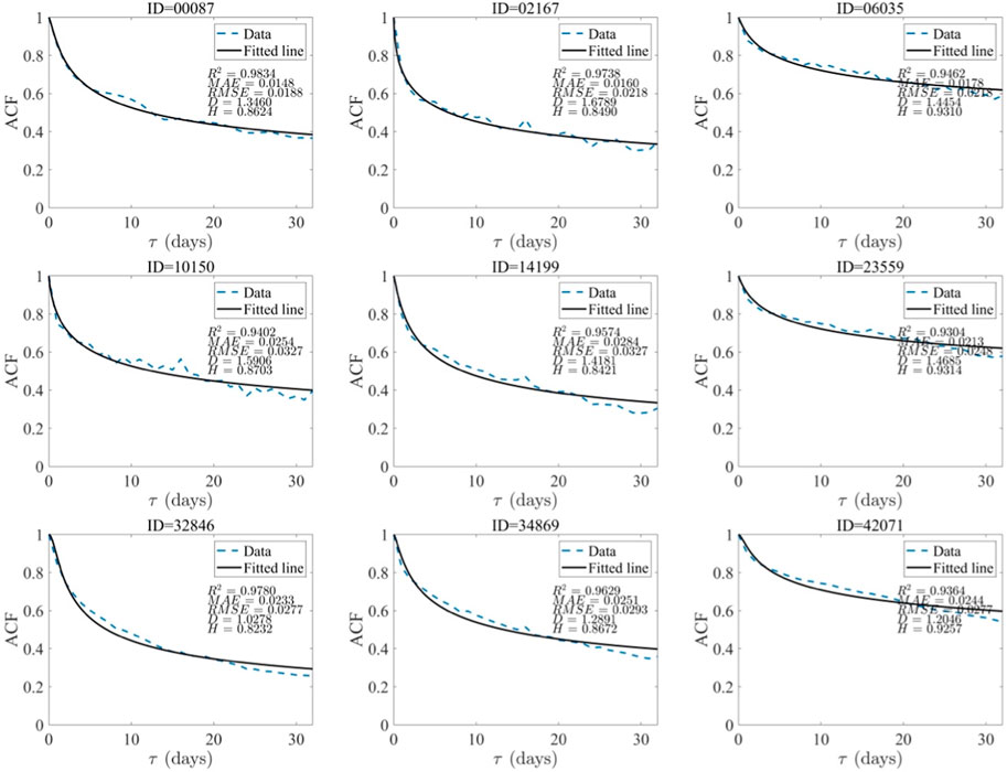
Figure 1. The empirical values (blue dashed line) and the theoretical generalized Cauchy model fitted values (black line) of the autocorrelation function of sea surface chlorophyll concentration.

Further, the fractal dimension and Hurst exponent, characterizing the self-similarity and long-term correlation characteristics of SSCC, were mapped by BME, shown in Figure 2. Figure 2A shows that high fractal dimension values are widely distributed in coastal areas of all continents, tropical areas of the North Pacific (except the areas near the equator), the areas of the South Pacific between 0 and 30 degrees, areas near 45 degrees in the South Pacific, areas between 15 and 25 degrees in the North Atlantic, and some regions of the Indian Ocean. Figure 2B shows that high Hurst exponent values are distributed around 30 degrees north and south latitudes in a belt-like pattern. The hot spot analysis made a step ahead for identifying high and low values aggregation areas of fractal dimension and Hurst exponent in a spatial distribution view, and the results are shown in Figure 3.

Figure 2

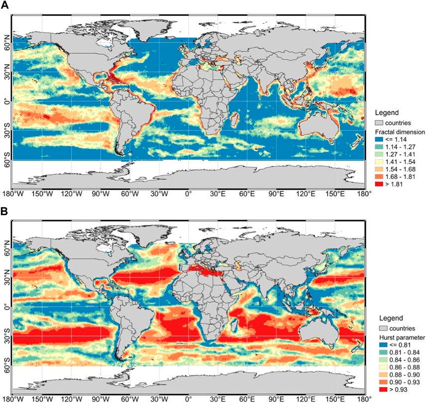
Figure 2. The spatial distributions of (A) fractal dimension and (B) Hurst exponent of the sea surface chlorophyll concentration globally.

Figure 3

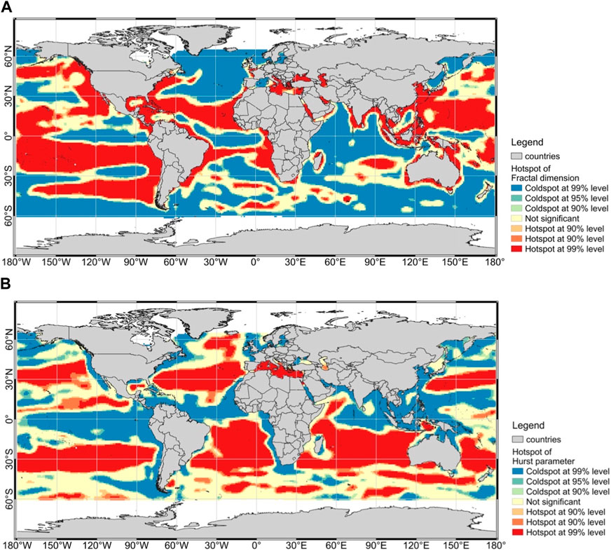
Figure 3. The hotspots of (A) fractal dimension and (B) Hurst exponent of the sea surface chlorophyll concentration globally.

3.3 Contributions of four sea surface parameters on hurst parameter and fractal dimension of SSCC

Although all environmental factors, i.e., sea surface height, sea surface salinity, sea surface temperature, sea surface wind, showed statistically significant with p values smaller than 0.001 in both univariate and multivariate GAM, the R square values of the univariate GAM are smaller than 0.2 and the R square values of multivariate GAM are vice versa. Regarding the generalized cross validation, the evaluation error of the univariate or multivariate GAM for modeling fractal dimension ranged from 0.0475 to 0.0584, while the corresponding error for modeling Hurst parameter ranged from 0.003 to 0.0034. The results of multivariate GAM and univariate GAM were presented in Figures 4, 5 and Appendix section, respectively. For fractal dimension of sea surface chlorophyll, the impacts of sea surface temperature and sea surface wind showed an overall increasing and decreasing trend, respectively; the impacts of sea surface height and sea surface salinity depicted an increasing-decreasing and fluctuating trend, respectively. Regarding the Hurst parameter of sea surface chlorophyll, the opposite trends of sea surface temperature and salinity impacts were detected; and similar decreasing-increasing-stable trends were found for the impacts of sea surface height and sea surface wind.

Figure 4

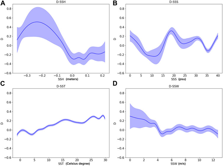
Figure 4. Partial dependences of (A) sea surface height, (B) sea surface salinity, (C) sea surface temperature, (D) sea surface wind on fractal dimension of sea surface chlorophyll using multivariate GAM model.

Figure 5

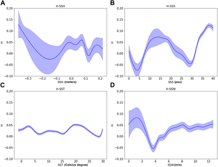
Figure 5. Partial dependences of (A) sea surface height, (B) sea surface salinity, (C) sea surface temperature, (D) sea surface wind on Hurst parameter of sea surface chlorophyll using multivariate GAM model.

4 Discussion

Compared with the Argo in-situ SSCC observations, the BME-generated SSCC product depicted more accuracy than the GlobColour product, indicating that the BME shows better performance than the DINEOF in SSCC interpolation. On the other hand, compared with the global SSCC distribution shown in the literatures [42,43], as well as the GlobColour product, the BME-generated SSCC product displays similar characteristics, including high- or low-values regions.

The spatial distributions of self-similarity and long-range correlation characteristics of global SSCC were explored for the first time in the current study. Generally, geostatistical methods are applicable to spatiotemporal analysis of natural attributes with strong spatiotemporal correlation [39,40,44]. This study found that BME will give high accurate prediction for SSCC, indicating that the SSCC may own strong spatiotemporal correlation, which is in line with Tobler’s First Law (the first law of geography): everything is related to everything else, but near things are more related than distant things [45]. Similar findings have been confirmed in many studies [15,28,30]. The outcome of this study is that the self-similarity and long-range dependence of SSCC have spatial correlation characteristics, varying in different regions. According to Figures 2, 3, the self-similarity and long-range dependence of SSCC are independent with each other, and their high- and low-value distributions are also inconsistent. On one hand, inland human activities often result in high nutrient burden along the coast forming eutrophic regions [43], which promotes algal growth and increase SSCC [46,47]; and it may be one of the reasons for the strong self-similarity characteristics of SSCC. Regarding the high fractal dimension values in the east coastal of United States, it was found that the river discharge from inland will have strong impacts on the circulation, salinity and water quality of the coastal regions of the New Jersey, Cape Hatteras and Florida, further influencing SSCC variations [48,49]. On the other hand, the Hurst exponent distribution indicating the strength of long-range dependence shows a similar distribution pattern to the values of SSCC [28], which suggests that areas with lower chlorophyll concentration or less nutrient-rich regions have more stable algal growth and relatively stable changes in SSCC, leading to stronger long-range dependence. For example, low primary production regions, oligotrophic regions, or the distribution of the depth of the 0.2 mm (ZNO₃) nitrate concentration showed similarities with the hot spots of Hurst parameter in the Pacific Ocean, Atlantic Ocean and Indian Ocean [43,50,51], as the mid-latitude regions (around 30°) in both hemispheres shown in Figure 3B. Moreover, the association between SSCC and sea surface temperature were also strong in these regions, while the distinct boundary located at around 45° latitude, which is due to the switch from negative to positive responses of SSCC to marine heatwaves [28,52].

Given the relatively weak self-similarity of SSCC, this discussion focuses solely on the long-range dependence of SSCC. The growth of phytoplankton is a continuous process that is influenced by environmental factors, such as nutrient concentration. The multivariate GAM results indicate that among the four factors, the sea surface height anomaly has the greatest influence on the long-range dependence of SSCC, as represented by the Hurst parameter (Figure 5). The sea surface height anomaly is associated with anticyclone- and cyclone-related eddies, which can transport nutrients from deeper sea layers to the surface, promoting phytoplankton growth [53–56]. The curve shown in Figure 5A demonstrates that cyclone-related eddies have a positive influence on the Hurst parameter, while anticyclone-related eddies have a negative influence. The contrasting impacts of sea surface temperature and salinity on the long-range dependence of SSCC, as shown in Figures 5B,C, result from the varying responses of different phytoplankton species or communities [57–61]. In other words, specific temperature and salinity conditions favor certain species or communities of phytoplankton, leading to their dominance and higher long-range dependence. Sea surface wind enhances mixing between surface and deeper waters, consequently impacting nutrient levels. Low wind speeds maintain favorable conditions for phytoplankton growth and keep SSCC at a relatively stable level. Strong winds with appropriate direction relative to the coast and hemisphere also contribute significantly to coastal upwelling, facilitating nutrient transport [35,62], thereby resulting in the high long-range dependence of SSCC observed in Figure 5D.

As the present study exclusively delved into examining the mono-fractal and long-range dependence characteristics of SSCC, future investigations could pivot towards the detection and quantification of multifractal features within SSCC, drawing inspiration from previous works [63–65]. Concurrently, an avenue for further exploration lies in dissecting the seasonal aspects of the long-range dependence and self-similarities inherent in SSCC, providing an opportunity for more comprehensive insights in future research. It should be acknowledged that the BME-generated SSCC at the north region of Russia may include uncertainty due to lack of remote sensing data (Supplementary Appendix A1, A2). Therefore, it is also worthy to find proper ways to improve the BME products at the polar regions in the future.

5 Conclusion

In the current study, the performance of BME on SSCC interpolation was evaluated as robust and effective with mean absolute error of cross validation equaling to 0.1295 mg/m³. The temporal variations of SSCC across the entire oceans were described using the generalized Cauchy model, and good performance was obtained with mean value of the R² equaling to 0.9141. The findings revealed strong long-range dependence and relatively weak self-similarity of SSCC; specifically, the values of Hurst parameter and fractal dimension ranged from 0.5 to 0.9632 and from 1 to 1.9484 with the mean values of 0.8667 and 1.2506, respectively. Further, the mid-latitude regions exhibited the highest long-range dependence, while the coastal regions showed the greatest self-similarity of SSCC. The use of GAM revealed that both sea surface height anomaly and sea surface wind made similar contributions to the long-range dependence of SSCC. Conversely, sea surface temperature and sea surface salinity had opposite effects on the long-range dependence of SSCC. Sea surface temperature is always positively correlated with the long-range dependence of SSCC.

Data availability statement

The original contributions presented in the study are included in the article/Supplementary Material, further inquiries can be directed to the corresponding author.

Author contributions

JH: Conceptualization, Formal Analysis, Funding acquisition, Methodology, Validation, Visualization, Writing–original draft, Writing–review and editing. ZG: Formal Analysis, Investigation, Methodology, Validation, Visualization, Writing–review and editing. YJ: Formal Analysis, Investigation, Methodology, Validation, Visualization, Writing–review and editing. ML: Conceptualization, Methodology, Resources, Writing–review and editing.

Funding

The author(s) declare that financial support was received for the research, authorship, and/or publication of this article. This work is supported by National Natural Science Foundation of China (Grant Nos. 42301374 and 42171398), the Zhejiang Provincial Natural Science Foundation of China (Grant No. LDT23D06024D06), National Key R&D Program of China (Grant No.2023YFE0113103), and HPC Center of Zhejiang University (Zhoushan Campus).

Acknowledgments

We would like to thank Mr Junjie Yin for his help on data pre-processing.

Conflict of interest

The authors declare that the research was conducted in the absence of any commercial or financial relationships that could be construed as a potential conflict of interest.

Publisher’s note

All claims expressed in this article are solely those of the authors and do not necessarily represent those of their affiliated organizations, or those of the publisher, the editors and the reviewers. Any product that may be evaluated in this article, or claim that may be made by its manufacturer, is not guaranteed or endorsed by the publisher.

Supplementary material

The Supplementary Material for this article can be found online at: https://www.frontiersin.org/articles/10.3389/fphy.2024.1331660/full#supplementary-material

References

1. Eppley RW, Stewart E, Abbott MR, Heyman U. Estimating ocean primary production from satellite chlorophyll. Introduction to regional differences and statistics for the Southern California Bight. J Plankton Res (1985) 7:57–70. doi:10.1093/plankt/7.1.57

CrossRef Full Text | Google Scholar

2. Longhurst A, Sathyendranath S, Platt T, Caverhill C. An estimate of global primary production in the ocean from satellite radiometer data. J Plankton Res (1995) 17:1245–71. doi:10.1093/plankt/17.6.1245

CrossRef Full Text | Google Scholar

3. Moore JK, Abbott MR. Phytoplankton chlorophyll distributions and primary production in the Southern Ocean. J Geophys Res Oceans (2000) 105:28709–22. doi:10.1029/1999JC000043

CrossRef Full Text | Google Scholar

4. Becker S, Tebben J, Coffinet S, Wiltshire K, Iversen MH, Harder T, et al. Laminarin is a major molecule in the marine carbon cycle. Proc Natl Acad Sci (2020) 117:6599–607. doi:10.1073/pnas.1917001117

PubMed Abstract | CrossRef Full Text | Google Scholar

5. Quinn PK, Bates TS, Schulz KS, Coffman DJ, Frossard AA, Russell LM, et al. Contribution of sea surface carbon pool to organic matter enrichment in sea spray aerosol. Nat Geosci (2014) 7:228–32. doi:10.1038/ngeo2092

CrossRef Full Text | Google Scholar

6. Jiao N, Wang H, Xu G, Aricò S. Blue carbon on the rise: challenges and opportunities. Natl Sci Rev (2018) 5:464–8. doi:10.1093/nsr/nwy030

CrossRef Full Text | Google Scholar

7. Raven J. Blue carbon: past, present and future, with emphasis on macroalgae. Biol Lett (2018) 14:20180336. doi:10.1098/rsbl.2018.0336

PubMed Abstract | CrossRef Full Text | Google Scholar

8. Bi H, Lu L, Meng Y. Hierarchical attention network for multivariate time series long-term forecasting. Appl Intell (2023) 53:5060–71. doi:10.1007/s10489-022-03825-5

CrossRef Full Text | Google Scholar

9. He X, Shi S, Geng X, Xu L, Zhang X. Spatial-temporal attention network for multistep-ahead forecasting of chlorophyll. Appl Intell (2021) 51:4381–93. doi:10.1007/s10489-020-02143-y

CrossRef Full Text | Google Scholar

10. Na L, Shaoyang C, Zhenyan C, Xing W, Yun X, Li X, et al. Long-term prediction of sea surface chlorophyll-a concentration based on the combination of spatio-temporal features. Water Res (2022) 211:118040. doi:10.1016/j.watres.2022.118040

PubMed Abstract | CrossRef Full Text | Google Scholar

11. Kettani H, Gubner JA. A novel approach to the estimation of the Hurst parameter in self-similar traffic. In: 27th Annual IEEE Conference on Local Computer Networks, 2002. Proceedings. LCN 2002. Presented at the 27th Annual IEEE Conference on Local Computer Networks, 2002. Proceedings. LCN 2002; November 6 2002 to November 8 2002; Tampa, FL, USA (2002). p. 160–5.

Google Scholar

12. Li M. Generalized fractional Gaussian noise and its application to traffic modeling. Physica A: Stat Mech its Appl (2021) 579:126138. doi:10.1016/j.physa.2021.126138

CrossRef Full Text | Google Scholar

13. Li M, Li J-Y. Generalized Cauchy model of sea level fluctuations with long-range dependence. Physica A: Stat Mech its Appl (2017) 484:309–35. doi:10.1016/j.physa.2017.04.130

CrossRef Full Text | Google Scholar

14. He J. Application of generalized Cauchy process on modeling the long-range dependence and self-similarity of sea surface chlorophyll using 23 years of remote sensing data. Front Phys (2021) 9:551. doi:10.3389/fphy.2021.750347

CrossRef Full Text | Google Scholar

15. He J, Christakos G, Wu J, Li M, Leng J. Spatiotemporal BME characterization and mapping of sea surface chlorophyll in Chesapeake Bay (USA) using auxiliary sea surface temperature data. Sci Total Environ (2021) 794:148670. doi:10.1016/j.scitotenv.2021.148670

PubMed Abstract | CrossRef Full Text | Google Scholar

16. Teoh KK, Ibrahim H, Bejo SK. Investigation on several basic interpolation methods for the use in remote sensing application. In: 2008 IEEE Conference on Innovative Technologies in Intelligent Systems and Industrial Applications. Presented at the 2008 IEEE Conference on Innovative Technologies in Intelligent Systems and Industrial Applications; 12-13 July 2008; Cyberjaya, Malaysia (2008). p. 60–5. doi:10.1109/CITISIA.2008.4607336

CrossRef Full Text | Google Scholar

17. Rossi RE, Dungan JL, Beck LR. Kriging in the shadows: geostatistical interpolation for remote sensing. Remote Sensing Environ (1994) 49:32–40. doi:10.1016/0034-4257(94)90057-4

CrossRef Full Text | Google Scholar

18. Jiang Q, He J, Wu J, Hu X, Ye G, Christakos G. Assessing the severe eutrophication status and spatial trend in the coastal waters of Zhejiang province (China): assessing the severe eutrophication status. Limnol Oceanogr (2019) 64:3–17. doi:10.1002/lno.11013

CrossRef Full Text | Google Scholar

19. Murphy RR, Curriero FC, Ball WP. Comparison of spatial interpolation methods for water quality evaluation in the chesapeake bay. J Environ Eng (2010) 136:160–71. doi:10.1061/(ASCE)EE.1943-7870.0000121

CrossRef Full Text | Google Scholar

20. Christakos G. A bayesian maximum-entropy view to the spatial estimation problem. Math Geology (1990) 22:763–77. doi:10.1007/BF00890661

CrossRef Full Text | Google Scholar

21. Christakos G, Li XY. Bayesian maximum entropy analysis and mapping: a farewell to kriging estimators? Math Geology (1998) 30:435–62. doi:10.1023/A:1021748324917

CrossRef Full Text | Google Scholar

22. He J, Christakos G. Bayesian maximum entropy. In: BS Daya Sagar, Q Cheng, J McKinley, and F Agterberg, editors. Encyclopedia of mathematical geosciences, encyclopedia of earth sciences series. Cham: Springer International Publishing (2021). p. 1–9. doi:10.1007/978-3-030-26050-7_50-1

CrossRef Full Text | Google Scholar

23. Yang Y, Christakos G. Spatiotemporal characterization of ambient PM 2.5 concentrations in shandong province (China). Environ Sci Technol (2015) 49:13431–8. doi:10.1021/acs.est.5b03614

PubMed Abstract | CrossRef Full Text | Google Scholar

24. Christakos G, Kolovos A. A study of the spatiotemporal health impacts of ozone exposure. J Expo Anal Environ Epidemiol (1999) 9:322–35. doi:10.1038/sj.jea.7500033

PubMed Abstract | CrossRef Full Text | Google Scholar

25. Cleland SE, West JJ, Jia Y, Reid S, Raffuse S, O’Neill S, et al. Estimating wildfire smoke concentrations during the october 2017 California fires through BME space/time data fusion of observed, modeled, and satellite-derived PM2.5. Environ Sci Technol (2020) 54:13439–47. doi:10.1021/acs.est.0c03761

PubMed Abstract | CrossRef Full Text | Google Scholar

26. Cobos M, Lira-Loarca A, Christakos G, Baquerizo A. Storm characterization using a BME approach. In: O Valenzuela, F Rojas, H Pomares, and I Rojas, editors. Theory and applications of time series analysis (2019). p. 271–84.

CrossRef Full Text | Google Scholar

27. He J, Christakos G, Jankowski P. Comparative performance of the LUR, ANN, and BME techniques in the multiscale spatiotemporal mapping of PM 2.5 concentrations in north China. IEEE J Sel Top Appl Earth Observations Remote Sensing (2019) 12:1734–47. doi:10.1109/JSTARS.2019.2913380

CrossRef Full Text | Google Scholar

28. He J, Christakos G, Cazelles B, Wu J, Leng J. Spatiotemporal variation of the association between sea surface temperature and chlorophyll in global ocean during 2002–2019 based on a novel WCA-BME approach. Int J Appl Earth Observation Geoinformation (2021) 105:102620. doi:10.1016/j.jag.2021.102620

CrossRef Full Text | Google Scholar

29. Hu B, Ning P, Li Y, Xu C, Christakos G, Wang J. Space-time disease mapping by combining Bayesian maximum entropy and Kalman filter: the BME-Kalman approach. Int J Geogr Inf Sci (2021) 35:466–89. doi:10.1080/13658816.2020.1795177

CrossRef Full Text | Google Scholar

30. He J, Chen Y, Wu J, Stow DA, George C. Space-time chlorophyll-a retrieval in optically complex waters that accounts for remote sensing and modeling uncertainties and improves remote estimation accuracy. Water Res (2020) 171:115403. doi:10.1016/j.watres.2019.115403

PubMed Abstract | CrossRef Full Text | Google Scholar

31. Zhao D, Gao L, Xu Y. Quantification of the impact of environmental factors on chlorophyll in the open ocean. J Ocean Limnol (2021) 39:447–57. doi:10.1007/s00343-020-9121-x

CrossRef Full Text | Google Scholar

32. Zhao N, Zhang G, Zhang S, Bai Y, Ali S, Zhang J. Temporal-spatial distribution of chlorophyll-a and impacts of environmental factors in the bohai sea and yellow sea. IEEE Access (2019) 7:160947–60. doi:10.1109/ACCESS.2019.2950833

CrossRef Full Text | Google Scholar

33. Desmit X, Ruddick K, Lacroix G. Salinity predicts the distribution of chlorophyll a spring peak in the southern North Sea continental waters. J Sea Res (2015) 103:59–74. doi:10.1016/j.seares.2015.02.007

CrossRef Full Text | Google Scholar

34. Garcia-Eidell C, Comiso JC, Berkelhammer M, Stock L. Interrelationships of sea surface salinity, chlorophyll-α concentration, and sea surface temperature near the antarctic ice edge. J Clim (2021) 34:6069–86. doi:10.1175/JCLI-D-20-0716.1

CrossRef Full Text | Google Scholar

35. Gao S, Wang H, Liu G, Li H. Spatio-temporal variability of chlorophyll a and its responses to sea surface temperature, winds and height anomaly in the western South China Sea. Acta Oceanol Sin (2013) 32:48–58. doi:10.1007/s13131-013-0266-8

CrossRef Full Text | Google Scholar

36. Chelton DB, Gaube P, Schlax MG, Early JJ, Samelson RM. The influence of nonlinear mesoscale eddies on near-surface oceanic chlorophyll. Science (2011) 334:328–32. doi:10.1126/science.1208897

PubMed Abstract | CrossRef Full Text | Google Scholar

37. Shafeeque M, Balchand AN, Shah P, George GBRS, Varghese E, Joseph AK, et al. Spatio-temporal variability of chlorophyll-a in response to coastal upwelling and mesoscale eddies in the South Eastern Arabian Sea. Int J Remote Sensing (2021) 42:4836–63. doi:10.1080/01431161.2021.1899329

CrossRef Full Text | Google Scholar

38. Ji C, Zhang Y, Cheng Q, Tsou J, Jiang T, Liang XS. Evaluating the impact of sea surface temperature (SST) on spatial distribution of chlorophyll-alpha concentration in the East China Sea. Int J Appl Earth Obs Geoinf (2018) 68:252–61. doi:10.1016/j.jag.2018.01.020

CrossRef Full Text | Google Scholar

39. Christakos G. Spatiotemporal random fields: theory and applications. Amsterdam, Netherlands: Elsevier (2017).

Google Scholar

40. He J, Kolovos A. Bayesian maximum entropy approach and its applications: a review. Stoch Environ Res Risk Assess (2018) 32:859–77. doi:10.1007/s00477-017-1419-7

CrossRef Full Text | Google Scholar

41. Li M. Long-range dependence and self-similarity of teletraffic with different protocols at the large time scale of day in the duration of 12 years: autocorrelation modeling. Phys Scr (2020) 95:065222. doi:10.1088/1402-4896/ab82c4

CrossRef Full Text | Google Scholar

42. Dierssen HM. Perspectives on empirical approaches for ocean color remote sensing of chlorophyll in a changing climate. PNAS (2010) 107:17073–8. doi:10.1073/pnas.0913800107

PubMed Abstract | CrossRef Full Text | Google Scholar

43. O’Reilly JE, Werdell PJ. Chlorophyll algorithms for ocean color sensors - OC4, OC5 and OC6. Remote Sensing Environ (2019) 229:32–47. doi:10.1016/j.rse.2019.04.021

CrossRef Full Text | Google Scholar

44. Wu J, He J, Christakos G. Quantitative analysis and modeling of earth and environmental data. Amsterdam, Netherlands: Elsevier (2021).

Google Scholar

45. Tobler WR. A computer movie simulating urban growth in the Detroit region. Econ Geogr (1970) 46:234–40. doi:10.2307/143141

CrossRef Full Text | Google Scholar

46. Harding LW, Mallonee ME, Perry ES, Miller WD, Adolf JE, Gallegos CL, et al. Long-term trends, current status, and transitions of water quality in Chesapeake Bay. Scientific Rep (2019) 9:6709. doi:10.1038/s41598-019-43036-6

PubMed Abstract | CrossRef Full Text | Google Scholar

47. Le C, Hu C, Cannizzaro J, English D, Muller-Karger F, Lee Z. Evaluation of chlorophyll-a remote sensing algorithms for an optically complex estuary. Remote Sensing Environ (2013) 129:75–89. doi:10.1016/j.rse.2012.11.001

CrossRef Full Text | Google Scholar

48. Boyer JN, Kelble CR, Ortner PB, Rudnick DT. Phytoplankton bloom status: chlorophyll a biomass as an indicator of water quality condition in the southern estuaries of Florida, USA. Ecol Indicators, Indicators Everglades Restoration (2009) 9:S56–S67. doi:10.1016/j.ecolind.2008.11.013

CrossRef Full Text | Google Scholar

49. Xu Y, Miles T, Schofield O. Physical processes controlling chlorophyll-a variability on the Mid-Atlantic Bight along northeast United States. J Mar Syst (2020) 212:103433. doi:10.1016/j.jmarsys.2020.103433

CrossRef Full Text | Google Scholar

50. Gregg WW, Rousseaux CS. Global ocean primary production trends in the modern ocean color satellite record (1998–2015). Environ Res Lett (2019) 14:124011. doi:10.1088/1748-9326/ab4667

CrossRef Full Text | Google Scholar

51. Signorini SR, Franz BA, McClain CR. Chlorophyll variability in the oligotrophic gyres: mechanisms, seasonality and trends. Front Mar Sci (2015) 2. doi:10.3389/fmars.2015.00001

CrossRef Full Text | Google Scholar

52. Noh KM, Lim H-G, Kug J-S. Global chlorophyll responses to marine heatwaves in satellite ocean color. Environ Res Lett (2022) 17:064034. doi:10.1088/1748-9326/ac70ec

CrossRef Full Text | Google Scholar

53. George TM, Manucharyan GE, Thompson AF. Deep learning to infer eddy heat fluxes from sea surface height patterns of mesoscale turbulence. Nat Commun (2021) 12:800. doi:10.1038/s41467-020-20779-9

PubMed Abstract | CrossRef Full Text | Google Scholar

54. Jiang L, Duan W, Wang H, Liu H, Tao L. Evaluation of the sensitivity on mesoscale eddy associated with the sea surface height anomaly forecasting in the Kuroshio Extension. Front Mar Sci (2023) 10. doi:10.3389/fmars.2023.1097209

CrossRef Full Text | Google Scholar

55. Liu Y, Zheng Q, Li X. Characteristics of global ocean abnormal mesoscale eddies derived from the fusion of sea surface height and temperature data by deep learning. Geophys Res Lett (2021) 48:e2021GL094772. doi:10.1029/2021GL094772

CrossRef Full Text | Google Scholar

56. Liu Y, Yu L, Chen G. Characterization of sea surface temperature and air-sea heat flux anomalies associated with mesoscale eddies in the South China sea. J Geophys Res Oceans (2020) 125:e2019JC015470. doi:10.1029/2019JC015470

CrossRef Full Text | Google Scholar

57. Butterwick C, Heaney SI, Talling JF. Diversity in the influence of temperature on the growth rates of freshwater algae, and its ecological relevance. Freshw Biol (2005) 50:291–300. doi:10.1111/j.1365-2427.2004.01317.x

CrossRef Full Text | Google Scholar

58. Flöder S, Jaschinski S, Wells G, Burns CW. Dominance and compensatory growth in phytoplankton communities under salinity stress. J Exp Mar Biol Ecol (2010) 395:223–31. doi:10.1016/j.jembe.2010.09.006

CrossRef Full Text | Google Scholar

59. Lomas MW, Glibert PM. Interactions between NH+4 and NO−3 uptake and assimilation: comparison of diatoms and dinoflagellates at several growth temperatures. Mar Biol (1999) 133:541–51. doi:10.1007/s002270050494

CrossRef Full Text | Google Scholar

60. Olli K, Ptacnik R, Klais R, Tamminen T. Phytoplankton species richness along coastal and estuarine salinity continua. The Am Naturalist (2019) 194:E41–E51. doi:10.1086/703657

PubMed Abstract | CrossRef Full Text | Google Scholar

61. Zeng J, Yin B, Wang Y, Huai B. Significantly decreasing harmful algal blooms in China seas in the early 21st century. Mar Pollut Bull (2019) 139:270–4. doi:10.1016/j.marpolbul.2019.01.002

PubMed Abstract | CrossRef Full Text | Google Scholar

62. Huynh H-NT, Alvera-Azcarate A, Beckers J-M. Analysis of surface chlorophyll a associated with sea surface temperature and surface wind in the South China Sea. Ocean Dyn (2020) 70:139–61. doi:10.1007/s10236-019-01308-9

CrossRef Full Text | Google Scholar

63. de Montera L, Jouini M, Verrier S, Thiria S, Crepon M. Multifractal analysis of oceanic chlorophyll maps remotely sensed from space. Ocean Sci (2011) 7:219–29. doi:10.5194/os-7-219-2011

CrossRef Full Text | Google Scholar

64. Umbert M, Guimbard S, Ballabrera Poy J, Turiel A. Synergy between ocean variables: remotely sensed surface temperature and chlorophyll concentration coherence. Remote Sensing (2020) 12:1153. doi:10.3390/rs12071153

CrossRef Full Text | Google Scholar

65. Umbert M, Hoareau N, Turiel A, Ballabrera-Poy J. New blending algorithm to synergize ocean variables: the case of SMOS sea surface salinity maps. Remote Sensing Environ Liege Colloquium Spec Issue Remote sensing ocean colour, temperature salinity (2014) 146:172–87. doi:10.1016/j.rse.2013.09.018

CrossRef Full Text | Google Scholar