HodgeRank as a new tool to explore the structure of a social representation

1 Introduction

The concept of social representation (SR) was introduced in social psychology by Moskovici in 1961 in a study of the social perception about psychoanalysis and consists of a framework of concepts, ideas, opinions, beliefs, or feelings shared by individuals in a given group, regarding a social object [1, 2]. Moskovici claimed that the theory of social representations “hopes to elucidate the links which unite human psychology with contemporary social and cultural questions” [3]. Since its introduction, the theory of SRs evolved both in its conceptual aspects and in the development of methodological tools to analyse data [4–6], and was applied to a broad range of social problems, including popular ideas about health and illness, the public understanding of science and new technologies, constructions of identities and human rights (see [7] and references therein). More recently, the theory has been applied in the study of media research [8], to social representations of the landscape [9], of court convictions on femicide [10], of environmental problems [11], of perceptions of illness treatments [12, 13], of perceptions of future [14], and several other social problems.

Two main problems in the context of the SRs theory consist in identifying the content and the structure of a social representation. The content of an SR can be understood as the set of cognitive elements shared by the group and relative to the social object—as said before, these elements can be opinions, knowledge, feelings, or beliefs —, whereas the structure describes how these elements are organised and how they interact with each other in the SR. The structure emerges from the social cooperation among the group members, which interact with each other, establishing some relationships between the cognitive elements. For a deep discussion about the structure of a SR see, for example, [5, 15, 16]. In the last decades, a great effort has been made in the development of quantitative tools, besides the more usual qualitative analysis, with the aim of investigating both the content and the structure of a social representation. In this regard, graphs of similarity, techniques of clustering, and statistical analysis of frequency and evocation rank are often used as methodological tools to study the content and structure of an SR (see [17], for instance, for a recent critical review of the methods used to study the structure of SRs).

One of the main conceptual tools in the study of the structure of a social representation is the central core theory, proposed by Abric in the 1970s [18]. According to this theory, the structure of an SR has two main characteristics, each one featuring two antagonist properties: the first one is to be “stable and moving, rigid and flexible,” and the second one is to be “consensual, but marked by strong individual differences” [15]. To cope with these two characteristics, the central core theory describes the structure of an SR employing a dual interacting system, formed by the central system and the peripheral system. The central system is formed by the cognitive elements that are highly stable, in the sense that they are resistant to changes, and have the function of strengthening the beliefs of the group, contributing to the continuity and consistency of the representation; at the same time, these elements share a significant consensus within the social group. On the other hand, the peripheral system is formed by less consensual (less shared) and less stable (less consistent) cognitive elements; this system is more heterogeneous, and absorbs the inter-individual differences, having a function of “protecting” the stability of the central system, by absorbing the inconsistencies or changes coming from the environment external to the social group. In this sense, it is said that the peripheral system contributes to making the central system stable [15, 16]. The interaction between these two systems characterises the dynamics of the structure of the social representation: some cognitive elements from one of these two systems eventually may move to another along the time, and these movements may cause a change in the social representation. These changes reflect, for instance, the change in the behaviour of the group members in order to adapt themselves to a new situation, knowledge, or information [16].

Several methods were proposed in the literature to study the content and the structure of a social representation. The main of these methods is based on word associations tasks [6, 17, 19]. In this method, people belonging to the social group under study are asked to evoke the words or expressions that come into their minds after the researcher presents them to an inducing word [19]. There are two main variants of this method. In the first, people freely evoke these words or expressions as they come into their mind. In the second variant, also known as hierarchical evocations, the researcher asks the respondents to rank the evoked words in order of importance [17, 19]. After collected, the words or expressions are typically put in a double-entry table, with four cells, organised according to the frequency of evocation and the average order of importance the respondents assigned to them [19, 20]. From such organisation, a group of words emerges as the most salient ones, which are those presenting a high frequency of evocation and a high average importance, as measured by the average evocation rank [19]. This method can access the content of the social representation but allows only to raise hypotheses about the centrality of the most salient words or expressions: the most salient words or expressions are said to be candidates to form the central core of the representation, and must be submitted to posterior tests to confirm or not the hypotheses of centrality [6, 17]. Another limitation of the double-entry table is that the thresholds used to delimit its four cells are somewhat ad hoc [17]. In this sense, it is said that the hierarchical word association allows to explore the structure of an SR since it only indicates a set of candidates to be after tested for centrality [6, 17, 19].

Despite its limitations, the hierarchical word associations method is very feasible, in the sense that it is based on a very simple procedure of data collection: the responden ts should be accessed just once to produce the individual set of a few ranked words; as a typical procedure, respondents are asked to evoke just five words. However, it would be desirable to combine the simplicity of the hierarchical word association method with a tool to extract information about the structure of the social representation that may prove to be more powerful than the usual Vergés’ double entry table. This is the main aim of the present work, in which we propose to apply the HodgeRank technique as a richer exploratory method to investigate the structure of a social representation. Here, we further refine and deepen the ideas of a preliminary work, authored by some of us, in which we first proposed to use the HodgeRank technique as a new quantitative tool in social representations theory [21].

HodgeRank is a very general technique based on the Hodge combinatorial theory, that allows building an optimal global ranking from incomplete and imbalanced pairwise ranking data [22–24]. The typical scenario in which the HodgeRank technique is useful is the following. Suppose that each individual within a group, which will be called a voter, ranks a set of objects pairwise, i.e., to each pair of objects considered by the voter, he or she compares one object against the other. As it is typical in modern datasets, the pairwise comparisons of each voter are highly incomplete, in the sense that just a few numbers of pairs of objects are compared by a typical individual. Moreover, the pairwise comparisons in the group are typically imbalanced, which means that some pairs are very often compared by the voters, whereas other pairs are rarely considered by the voters. For example, a customer may rate some films she/he watched on Netflix, in such a way that a direct comparison can be inferred between each pair of films she/he rated. But, of course, a typical customer will not rate all the films in the platform, and, thus, their pairwise comparison will be imbalanced. The notions of “voters” and “objects” are very general, and can be adapted to several contexts. For examples of application of HodgeRank in different problems, see [23, 25, 26]. The features of incompleteness and imbalance of pairwise comparisons fit very well with the kind of data typically collected from hierarchical word association tasks, where each member (a voter) of the social group ranks a few number of words or expressions that he or she associates with the inducing word. The ranking of these few words can be reinterpreted as pairwise rankings, in which the first ranked word is preferred over each of the other evoked words; the second word is preferred over the third, the fourth, and so on. Moreover, within a social group, there will be certain pairs of words that will be compared by several voters, and other pairs that will be compared by a relatively small number of voters. As we will discuss later, this feature is intimately linked to the existence of a central and a peripheral structure in the SR.

The HodgeRank technique starts from the individual pairwise comparisons and builds, in the end, an optimal global ranking of all the objects within the group; the optimal global ranking is that global ranking which is “closer,” in a sense that will become clear later, to the individual pairwise rankings. As we will show in this paper, when we apply the HodgeRank technique to SRs, a structure emerges very naturally, since the HodgeRank outcomes can be represented by a graph with a structure analogous to that of an electrical circuit, in which each word corresponds to an electrical node on which is applied an electrical potential (the word’s global rank). Moreover, to each pair of nodes (words) will correspond, in the electrical analogy, an electric current, when the corresponding words have a direct comparison between themselves.

Besides providing a global ranking and a static description of the structure of the SR, the HodgeRank technique also allows us to identify the sources of inconsistencies in the global ranking. We shall interpret such inconsistencies as instabilities of the global ranking and, therefore, as potential drivers for the dynamical changes in the structure of the SR along the time. The identification of these dynamic drivers may be useful when the SR is considered from the point of view of a dual interacting system [16, 17].

This paper is organised as follows. In Section 2.1 we present the classical method of construction of the Vergés’ double entry table from data collected by a hierarchical word association task, with the inducing word “COVID-19,” applied to two social groups, one of them formed by faculty members and the other formed by students, both of them from higher education institutions in Brazil. After building the double entry table, we will discuss some of the limitations of this method, especially regarding the exploration of the SR structure and dynamics. In Section 2.2 we briefly present the main ideas of the HodgeRank technique, with emphasis on obtaining the optimal global ranking, the identification of the graph structure and its analogy with an electrical circuit, and the identification of the sources of inconsistencies in the global ranking. In Section 3.1 we apply the HodgeRank technique on the same data used to build the double entry table of Section 2.1, and discuss the kind of new information we obtain from this methodology. In particular, we emphasise the possibility of identifying the sources of the ranking inconsistencies directly on the graph, and the possibility of guessing the drivers for changes in the SR structure over time. Finally, in Section 4 we present our conclusions.

2 Methods

2.1 Two social representations of COVID-19 among students and faculty members of Brazilian higher education institutions

Before presenting the HodgeRank technique, we will first present the classical construction of a Vergés’ double-entry table with data collected according to the hierarchical word association method, with the aim of identifying the social representation of COVID-19 within two social groups belonging to higher education institutions (HEIs) in Brazil, including universities, colleges and federal institutes. One of these groups was formed by students (from undergraduate and graduate courses) and the other was formed by faculty members.

The data were collected by the authors by sending electronic questionnaires (Google Forms) to students and faculty members of HEIs over all the Brazilian territory, during the period from November 2020 to May 2021, when the classes were given remotely as one of the local government’s measures to prevent the dissemination of SARS-CoV-2. Among other questions, which are not being considered in the present work, each individual was asked to answer the following: “cite the five first words that come to your mind, ranked in order of importance, that best represent the term COVID-19.” A total of 729 students and 424 faculty members voluntarily replied to the questionnaires. In the group of students, 20% came from private, 26% from municipal, 31% from state and 23% from federal HEIs. In the group of faculty members, 11% were from private, 6% from municipal, 36% from state and 47% from federal HEIs. The respondents came from all the Brazilian Regions, even if the proportions of respondents in the sample did not represent accurately the proportions of the students of faculty members in their respective regions. Only four States of the Northern Region were absent in the sample, with no respondent (Acre, Amazonas, Rondonia, Roraima and Tocantins).

After the data collection, we assigned the scores 1 to 5 to each word evoked by an individual, with 1 being assigned to the most important and 5 to the less important one. As a second step, for each social group, we have made a catalogue with all the cited words and merged them under a single representative word, or category, those words having very close meanings. Here, in order to minimize the subjectivity in this procedure, two of the authors independently did the merging procedure; after that, they analysed and discussed together the divergences in their results until a consensus was obtained. Although such a categorisation procedure is somewhat standard in the SR literature, it is one of the weaknesses of the method of word associations, since it is not immune to subjective biases in grouping the words based on their “semantic proximity.” For a critic discussion about the limitations and weakness of the categorisation procedure in word associations tasks, see [6, 17]. In this work we will not focus at this stage of the data preparation, and will apply the HodgeRank on the data already categorised. However, it would be interesting to explore, in future works, the possibility to perform this categorisation with the aid of more objective methods, such as grouping the words by using the distances between them, as measured, for insance, in the WordNet database [27], or by using word embeddings techniques such as Word2vec [28].

After the categorization procedure, the resulting set of words for each social group was organised in a double-entry table, with four cells [17, 20]. In this table, the two upper cells contain the words (categories) that were cited (or evoked) most frequently. The frequency associated with a word (category) is the proportion of individuals in the group that evoked that word. The two left cells contain the words best ranked, on average. The average evocation rank (AER) of a word is simply the average of the scores that word received within the social group. To delimit the four cells we used, as usual in the literature of SR, a threshold of 15% to separate the upper from the lower cells, and a threshold of 3 in the AER to separate the left from the right cells. Our results are shown in Tables 1, 2, where we did not include words whose frequencies were equal to or below the first tercentile of the frequencies; words below this threshold were considered poorly representative within the social group.¹

Table 1

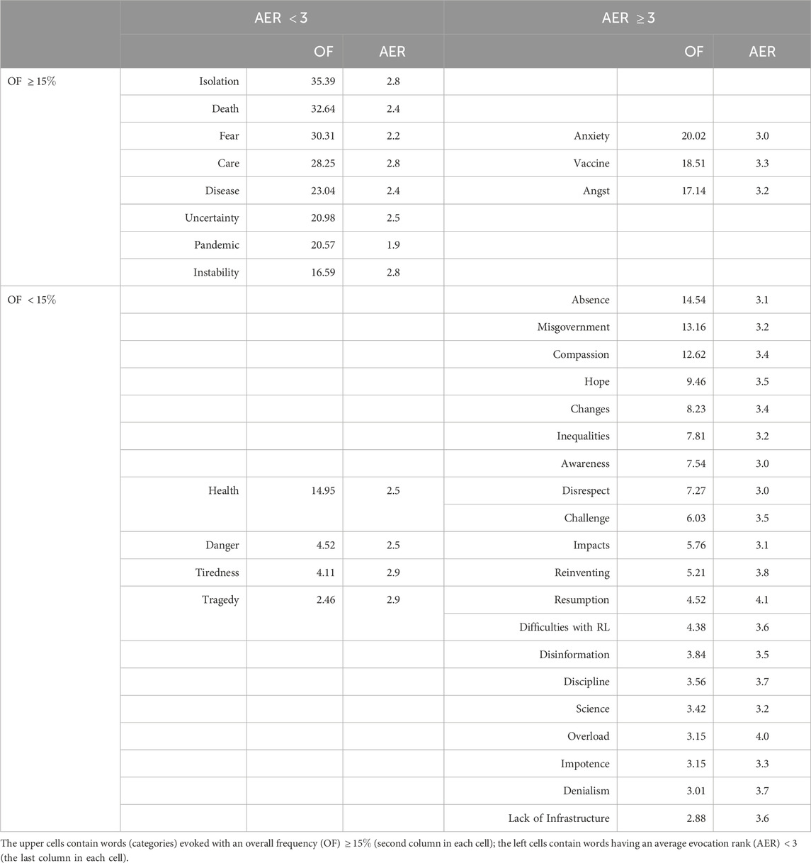
Table 1. Vergés’ double-entry table for the SR of COVID-19 in a group of students from higher education institutions in Brazil.

Table 2

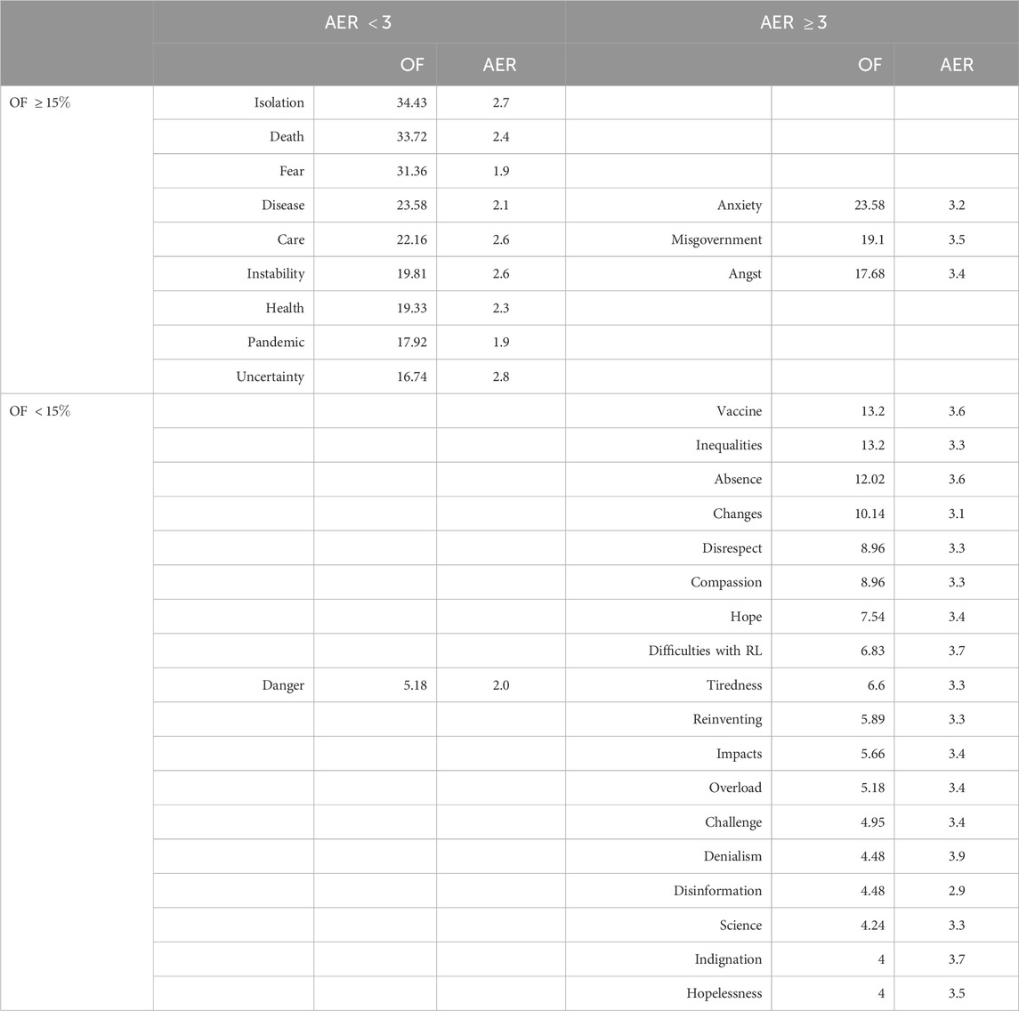
Table 2. Same as Table 1 for the group of faculty members.

The double-entry Tables 1, 2 identify the most salient elements of the representation, which are the words most frequently cited and with a lower average (higher importance) evocation rank. These are the words located at the upper left cell, and they constitute themselves as the “candidates for the central core” [16, 17]. Additional tests are needed to identify which of these candidates actually belong to the central core; the double-entry table allows one only to raise a conjecture about the potential candidates to the central core and does not provide us with much more information about the structure of the social representation. An evident limitation to interpreting the results organised in a double-entry table is the somewhat ad hoc specification of the threshold values for the frequency and the AER, which were used to determine the boundaries of the four cells. On the other hand, a clear advantage of the method of hierarchical associations is that it is very simple in what regards the data collection: only a single access to the population is needed and, in this respect, we can say that it is very feasible in what regards the field research [17].

In the next sections, we propose the use of the HodgeRank technique as a tool to deepen further the exploration of the data collected in the hierarchical word association method. Even if the HodgeRank is still an exploratory tool, we will show that it does provide more complex information than Vergés’ double-entry table, especially in what concerns the exploration of the structure of the social representation. The HodgeRank outcomes will be represented by a graph, analogous to the graph of an electrical circuit which, besides providing a global ranking of the words within each group, reveals a structure among the words; this structure is associated with the relative importance between the words in each pair, as well as a measure of the consensus of the pairwise comparisons. Another useful outcome of the HodgeRank technique is the identification of the inconsistencies of the actual answers within the group concerning the global ranking; by properly interpreting such inconsistencies we may guess which are the potential drivers for the dynamics in the SR structure, i.e., which are the cognitive elements more likely to move between the central and the peripheral systems along the time.

2.2 Some basic concepts on the combinatorial Hodge theory and the HodgeRank technique

In this section, we will present the basic concepts behind the HodgeRank technique. Even if this presentation is somewhat technical in what regards to the mathematical aspects of the method, the application of it to a data set is very simple. In the Appendix, we present a pseudocode to illustrate the main steps to identify the inconsistencies. The electric analogous of the graph structure can be built straightforwardly by using the global ranking and the adjacency matrix. A complete code written in the Wolfram Language^© will be freely available under request to the authors.

2.2.1 Elements of the combinatorial Hodge theory

We start by recalling some basic concepts on graphs. A finite (undirected) graph G is defined as a pair of two sets, G = (V, E), where V is the set of vertices and $E\subseteq \left(\begin{array}{c}\hfill V\hfill \\ \hfill 2\hfill \end{array}\right)$ is the set of edges. Here the symbol $\left(\begin{array}{c}\hfill V\hfill \\ \hfill 2\hfill \end{array}\right)$ denotes the family of all the binary subsets of V. In the applications, V is the set of the objects we wish to rank. In this work, V is the set of all words or expressions (after categorization) evoked by the members of the social group. The elements of the set E will be all the pairs of words (categories) that were evoked by at least one individual. Here we will sometimes use the notation G(V, E) to recall the sets V and E that define the graph G. If n is the number of elements (vertices) in V, we will label them by integer numbers, i.e., V = {1, 2, …, n}. If i, j ∈ V and {i, j} ∈ E, then we say that the vertices i and j are linked by an edge; otherwise, this pair of vertices are said to be not linked, or that the corresponding edge is absent in the graph. A useful way to visualize a graph is by representing its vertices by points and its edges by line segments linking the corresponding vertices. In our application to a social representation, the vertices are the words and the edges represent that at least one individual “compared” the two corresponding words. The adjacency matrix a = [a_ij] (i, j ∈ V) associated to a graph G(V, E) is a square matrix whose elements are a_ij = 1 if {i, j} ∈ E, and zero otherwise. It is also possible to attribute weights $\omega :V\times V\to {\mathbb{R}}_{+}$ to all the pairs of vertices of a graph, such that ω_ij = ω_ji > 0, if {i, j} ∈ E, and zero otherwise. Thus, a_ij = 1 if ω_ij ≠ 0, and a_ij = 0 otherwise. Furthermore, in addition to the sets V and E, we can define another one, called the set of triangles (or 3-cycles) of G(V, E), denoted by T(G), such that {i, j, k} ∈ T(G) if {i, j}, {j, k}, {k, i} ∈ E.

Given a finite graph G, we can define suitable functions on the sets V, V², and V³. For instance, let $r:V\to \mathbb{R}$ be any function that associates a real number to each vertex. Moreover, we call an alternating function on the edges any function $X:V\times V\to \mathbb{R}$, that satisfies X_ij = −X_ji for all {i, j} ∈ E and X_ij = 0 if {i, j}∉E. We also can define an alternating function on the triangles as a function $\mathrm{\Phi }:V\times V\times V\to \mathbb{R}$ such that Φ_ijk = Φ_jki = Φ_kij = −Φ_jik = −Φ_ikj = −Φ_kji for all {i, j, k} ∈ T(G), and Φ_ijk = 0 otherwise. We use the sub-index notation for the values of these functions, like r_i, X_ij, and Φ_ijk, instead of the usual function notation (like r(i), X(i, j), Φ(i, j, k)), since the indices are discrete. Once such functions can be represented, respectively, by column, square, and cubic hypermatrices, we can associate to a graph G(V, E) the following vector spaces [22]

$\begin{array}{ccc}\hfill & \hfill & C^0=\left\{r|r:V\to \mathbb{R}\right\}\hfill \\ \hfill & \hfill & \hfill \\ \hfill & \hfill & C^1=\left\{X|X:V\times V\to \mathbb{R}\text{is\hspace{0.17em}an\hspace{0.17em}alternating\hspace{0.17em}function\hspace{0.17em}on\hspace{0.17em}}E\right\}\hfill \\ \hfill & \hfill & \hfill \\ \hfill & \hfill & C^2=\left\{\mathrm{\Phi }|\mathrm{\Phi }:V\times V\times V\to \mathbb{R}\text{is\hspace{0.17em}an\hspace{0.17em}alternating\hspace{0.17em}function\hspace{0.17em}on\hspace{0.17em}}T\left(G\right)\right\}.\hfill \end{array}(1)$

The space C⁰ is called the space of potential functions, C¹ is the space of edge flows, and C² is the space of triangle flows. In the topological jargon, the elements of the vector spaces C⁰, C¹, and C² are called 0-, 1-, 2-cochains, respectively.

For the ranking procedure, we need to equip the vector spaces described above (Eq. 1) with suitable inner products. There are different ways to define consistent inner products in a vector space; here we use the most common choices [23]:

$\langle r,{s\rangle }_0={\displaystyle \sum _{i=1}^n}{r}_i{s}_i,\mathrm{f}\mathrm{o}\mathrm{r}r,s\in C^0,\langle X,{Y\rangle }_1={\displaystyle \sum _{i<j}}{w}_{ij}{X}_{ij}{Y}_{ij},\mathrm{f}\mathrm{o}\mathrm{r}X,Y\in C^1,(2)$

and

${⟨\mathrm{\Phi },\mathrm{\Theta }⟩}_2={\displaystyle \sum _{i<j<k}}{\mathrm{\Phi }}_{\mathit{ijk}}{\mathrm{\Theta }}_{\mathit{ijk}},\mathrm{f}\mathrm{o}\mathrm{r}\mathrm{\Phi },\mathrm{\Theta }\in C^2.(3)$

The inner products in C⁰ and C² are just the familiar Euclidean inner products. The reason for choosing a weighted inner product in C¹ will be justified later when we discuss the optimization procedure which will lead to the global ranking of the objects in V.

Based on such inner products we also define the following special linear operators acting between these spaces (called coboundary operators):

$\mathbf{g}\mathbf{r}\mathbf{a}\mathbf{d}:C^0\to C^1,\mathrm{w}\mathrm{i}\mathrm{t}\mathrm{h}{\left(\mathbf{g}\mathbf{r}\mathbf{a}\mathbf{d}r\right)}_{ij}=a_{ij}\left(r_j-r_i\right);(4)$

$\mathbf{d}\mathbf{i}\mathbf{v}:C^1\to C^0,\mathrm{w}\mathrm{i}\mathrm{t}\mathrm{h}{\left(\mathbf{d}\mathbf{i}\mathbf{v}X\right)}_i={\displaystyle \sum _{j=1}^n}{w}_{ij}{X}_{ij};(5)$

$\mathbf{c}\mathbf{u}\mathbf{r}\mathbf{l}:C^1\to C^2,\mathrm{w}\mathrm{i}\mathrm{t}\mathrm{h}{\left(\mathbf{c}\mathbf{u}\mathbf{r}\mathbf{l}X\right)}_{\mathit{ijk}}=t_{\mathit{ijk}}\left(X_{ij}+X_{jk}+X_{ki}\right).(6)$

In the above expressions i, j, k ∈ V, a_ij are the elements of the adjacency matrix and t_ijk = a_ija_jka_ki, i.e., t_ijk = 1 if {i, j, k} ∈ T(G), and t_ijk = 0 otherwise. The above special operators are the (combinatorial) gradient, divergent, and curl operators, and are discrete analogues of the gradient, divergent, and curl operators appearing in vector calculus.

With the inner products defined before we can find the adjoints of these operators, which are defined in the usual way, i.e., if we make k = 0, 1, then if δ_k: C^k → C^k+1 and ${⟨{\delta }_k{f}_k,g_{k+1}⟩}_{k+1}={⟨f_k,{\delta }_k^{*}{g}_{k+1}⟩}_k$, for all f_k ∈ C^k and all g_k+1 ∈ C^k+1, then ${\delta }_k^{*}:C^{k+1}\to C^k$ is the adjoint of δ_k. Therefore, we have that div = −grad*, as it happens in vector calculus [22]. Also, it is natural to define the Laplacian operator, Δ₀: C⁰ → C⁰, as Δ₀ = −div grad and the Helmholtz operator, Δ₁: C¹ → C¹, as Δ₁ = −grad div + curl* curl. So we have that Δ₀ = grad* grad and Δ₁ = grad grad* + curl* curl. In summary, we can go from a certain cochain to another cochain using operators like the scheme presented in Figure 1. Since we represent a function r as a vector of n entries, where n is the number of vertices in V, X can be represented as a n × n matrix and Φ as a n × n × n hypermatrix. Thus, in matrix notation, div X is also a vector of n entries, while Δ₀ is an n × n matrix and so on.By using the above operators the space of edge flows C¹ can be decomposed as an orthogonal sum

$C^1=\mathrm{i}\mathrm{m}\left(\mathbf{g}\mathbf{r}\mathbf{a}\mathbf{d}\right)\oplus \mathrm{k}\mathrm{e}\mathrm{r}\left({\mathrm{\Delta }}_1\right)\oplus \mathrm{i}\mathrm{m}\left({\mathbf{c}\mathbf{u}\mathbf{r}\mathbf{l}}^{*}\right),(7)$

where the symbol im stands for the image of an operator, and ker stands for its kernel. The above decomposition is called Helmholtz decomposition for graphs [23]. It means that for any edge flow X ∈ C¹, there exist $\tilde{s}\in C^0,\mathrm{\Phi }\in C^2$ and h ∈ C¹, with Δ₁ h = 0, such that X can be decomposed in a unique way as

$X=\mathbf{g}\mathbf{r}\mathbf{a}\mathbf{d}\tilde{s}+h+{\mathbf{c}\mathbf{u}\mathbf{r}\mathbf{l}}^{*}\mathrm{\Phi }.(8)$

This decomposition will be crucial in interpreting the results of the global rankings we will obtain, as well as the nature of its inconsistencies.

Figure 1

Figure 1. Cochains and operators scheme.

2.2.2 The HodgeRank technique

As we mentioned earlier, the data collected in the hierarchical word association tasks are typically incomplete and imbalanced. There is also an implicit graph structure arising from (incomplete) pairwise comparisons. Below we explain in more detail such terms and introduce some notations.

Let us label the individuals (“voters”) within a social group by the index α. The quantity $r_i^{\alpha }$ is the order (or the “rank,” or the “score”) the voter α assigned to the word i. In our data, the scores that a given individual assigns for the set of few evoked words will be all different, and assume integer values from 1 to 5, since each individual is asked to rank just five words, in order of importance. With the set of scores of the voter α in hand, we associate a measure $Y_{ij}^{\alpha }$ for the relative importance this voter assigns to the pair of words i and j. Such measurement can be defined in different ways. Here we use the score differences, which is the most usual choice: $Y_{ij}^{\alpha }=r_j^{\alpha }-r_i^{\alpha }$, if the individual α evokes both the words i and j, and zero otherwise. Obviously, $Y_{ij}^{\alpha }=-Y_{ji}^{\alpha }$. Other possible choices would be choosing the binary comparison or the logarithm of score ratios, defined, respectively, as $Y_{ij}^{\alpha }=\mathrm{s}\mathrm{i}\mathrm{g}\mathrm{n}\left(r_j^{\alpha }-r_i^{\alpha }\right)$ or $Y_{ij}^{\alpha }=\log r_j^{\alpha }-\log r_i^{\alpha }$ if α compares i and j, and zero otherwise [23]. Anyway, if $r_i^{\alpha }<r_j^{\alpha }$, then the individual assigned a higher importance to i than to j and $Y_{ij}^{\alpha }$ will be positive. In our application, the quantity $Y_{ij}^{\alpha }$ thus measures the intensity of the differences of importance the individual α assigns to the words i and j. To cope with the usage in the literature, we will refer to $Y_{ij}^{\alpha }$ as the pairwise comparison between the words i and j made by the individual α. In Section 3.1 we show that different choices for the specific form of $Y_{ij}^{\alpha }$ will lead essentially to the same results for the global ranking and the measure of the inconsistencies. Therefore, the specific choice for $Y_{ij}^{\alpha }$ is not a matter of concern.

In general, each individual makes a highly incomplete number of pairwise comparisons. This is especially true in our application, where the researcher asks each individual to rank only five words, in order of importance. In this case, we interpret each individual answer as giving all the possible pairwise comparisons between all the pairs taken from those five words, which is just a small subset of the complete set of words (or categories) evoked by the set of all the members of the social group.² In order to deal with the incompleteness of individual pairwise comparisons, and to obtain a single graph of pairwise comparisons that represents the whole social group, we will aggregate all the individual pairwise comparisons. The resulting graph generally will not be a complete graph but will be much less sparse than the corresponding individual graphs of pairwise comparisons. There are also diverse possible choices to do this aggregation. Here we will use the most natural choice, which corresponds to associating each pair of words (in the full set of words) with the average pairwise comparison:³

$Y_{ij}=\frac{1}{{\omega }_{ij}}{\displaystyle \sum _{\alpha }}{Y}_{ij}^{\alpha },(9)$

if ω_ij > 0, where ω_ij is the number of individuals that compared the objects i and j. If no individual compared these two objects, then ω_ij = 0 and, in this case, we define Y_ij = 0.

To the above form of aggregation of individual pairwise comparisons, we associate a weighted graph G(V, E), called the pairwise comparison graph, where V is the set of all the words (categories) evoked by the subjects within the social group, and $E=\left\{\{i,j\}|i,j\in V\right.$ and $\left.{\omega }_{ij}>0\right\}$. The matrix ω = [ω_ij = ω_ji], i, j ∈ V, is the matrix of edge weights. The adjacency matrix of this graph is a = [a_ij], i, j ∈ V, where a_ij = 1 if ω_ij ≠ 0, and a_ij = 0 otherwise. From now on we will assume that the graph G(V, E) is connected. If G(V, E) were not connected, we should conclude that the social group was not well characterised, since, for instance, there would be at least two subgroups of individuals with no shared idea, concept, feeling, or belief; such subgroups should not be considered as subsets of a well characterised social group.

As mentioned above, the graph G(V, E) generally is not a complete graph. The remaining incompleteness of the aggregated pairwise comparisons is still manifest in the edge sparsity: several pairs of words will still not be compared in the aggregated graph, because these pairs were not compared by any individual in the social group. On the other hand, the imbalance of the data will correspond, in the graph structure, to a nonuniform distribution for the vertices’ strengths. The strength d_i of the vertex (word) i is the sum of the weights of the edges incident on it, i.e., $d_i={\sum }_{j=1}^n{\omega }_{ij}$, where n is the number of words/categories in the vertex set V. In our application, d_i is just the total number of pairwise comparisons in which the word i appears. In fact, some words will appear in the pairwise comparisons within the group much more frequently than others and, therefore, will have a strength much greater than others. None of these features (incompleteness and imbalance) is a problem for the HodgeRank method. In fact, we will show that the method provides a suitable way to deal with both of these features of the data.

Now, it is straightforward to see that the matrix $Y=\left[Y_{ij}\right]=-\left[Y_{ji}\right],i,j\in V$, introduced in Eq. 9, indeed defines an edge flow, and thus Y ∈ C¹, according to Eq. 1. However, this edge flow Y will almost certainly be inconsistent, and will not be associated with a global ranking. The reason is that, as known in many theoretical and empirical social studies, the data is probably plagued with triangle or cyclic inconsistencies. For instance, if, in the aggregate pairwise comparison graph, we have a word i that is preferred against a word j (Y_ij > 0) and that word j is preferred against the word k (Y_jk > 0), but, by its turn, the word k is preferred against the first word i (Y_ki > 0), then we say that the aggregate pairwise comparisons regarding the words in the triangle {i, j, k} are inconsistent; in this case, we have that Y_ij + Y_jk + Y_ki ≠ 0, with {i, j, k} ∈ T(G). On the other hand, if Y_ij + Y_jk + Y_ki = 0 for {i, j, k} ∈ T(G), then we say that the pairwise comparisons in the triangle {i, j, k} ∈ T(G) is consistent. Later we will define precisely what we mean by triangle and cyclic inconsistencies and will see that by using the Helmholtz orthogonal decomposition Eq. 8 it is possible to extract a component of Y, called the gradient flow, that is free of such inconsistencies, and thus this component will correspond to a consistent ranking.

In the idealistic situation in which there is no inconsistency in the set of observed pairwise comparisons Y_ij, one may seek for a “potential” function $s:V\mapsto \mathbb{R}$ (which will define a “global ranking”) such that

$Y_{ij}=a_{ij}\left(s_j-s_i\right)={\left(\mathbf{g}\mathbf{r}\mathbf{a}\mathbf{d}s\right)}_{ij},(10)$

where a_ij are the elements of the adjacency matrix of the aggregate pairwise comparison graph G(V, E). Observe that solving the above equation to find such a potential is analogous to seeking the electric potential in each node of an electric circuit when we know the electric currents flowing between each pair of nodes. In such analogy, the electric nodes i and j are linked by an electric conductor having an electric admittance (the inverse of the electric resistance) equal to a_ij, which here can assume only two possible values, 1 or 0; if a_ij = 0 the two nodes are isolated from each other (i.e., the resistance between the two nodes is infinite). Here we are assuming the convention that the electric current Y_ij flows from node i to node j if the electric potentials satisfy s_i < s_j.

In the more realistic situation, and due to the personal character of the answers given to the researcher, inconsistencies in the set of edge flows Y_ij will always be expected, and a solution s_i, as above, may not exist for a pairwise comparison graph G(V, E). Nevertheless, one can seek for the “best” solution $\tilde{s}$ (that will correspond to the global ranking we are searching for) such that $Y_g\equiv \mathbf{g}\mathbf{r}\mathbf{a}\mathbf{d}\tilde{s}$ is as close as possible to the empirically observed Y. More precisely, the set of weights w_ij yields an inner product in the space of edge flows C¹ and one seeks the orthogonal projection of the edge flow Y into the subspace of C¹ containing all the gradient flows, i.e., into $\mathrm{i}\mathrm{m}(\mathbf{g}\mathbf{r}\mathbf{a}\mathbf{d})=\left\{X\in C^1|X=\text{grad\hspace{0.17em}}s,\text{for\hspace{0.17em}some\hspace{0.17em}}s\in C^0\right\}$. Therefore, the problem reduces to the classical least squares problem, in which we seek for Y_g ∈ im(grad) such that the squared norm of the difference Y_g − Y, i.e.,

${\left|\left|Y_g-Y\right|\right|}_1^2\equiv {⟨Y_g-Y,Y_g-Y⟩}_1={\displaystyle \sum _{i<j}}{\omega }_{ij}{\left[{\left(Y_g\right)}_{ij}-Y_{ij}\right]}^2(11)$

is a minimum. Above, $\Vert \cdot {\Vert }_1^2$ is the squared norm in the space C¹.⁴ With our definition of the inner product in Eq. 2, the least squares method takes naturally into account the different edges according to their weights, with a greater relevance attributed to the heaviest edges. In our application here, this means that pairs of words that were compared by a greater number of individuals have a greater influence in determining the optimal global ranking.

Now we describe our algorithm to obtain the three components in the Helmholtz decomposition (Eq. 8) (the corresponding pseudocode is given in the Appendix). The first step consists of fixing an ordering for the vertices, edges, and triangles in the graph. One also needs to choose orientations for edges and triangles in the graph (technically, we need to construct an oriented 2-complex). However, the final results of our calculations do not depend on our choices for such orientations.

The chosen orderings for vertices, edges, and triangles allow us to construct matrix representations for the curl and grad operators and to represent Y by a column matrix (vector), instead of a square matrix. Then we can write the Helmholtz decomposition as

$Y=Y_g+Y_h+Y_c,(12)$

where Y is the (generally inconsistent) empirically observed pairwise ranking, Y_g ∈ im(grad), Y_c ∈ im(curl*), and $Y_h\in \mathrm{k}\mathrm{e}\mathrm{r}\left({\mathrm{\Delta }}_1\right)$. In our algorithm, Y, Y_g, Y_h, and Y_c will all be represented by column matrices (vectors), not square matrices. The matrix representation of the operator curl has a number of rows equal to the number of triangles in the graph and a number of columns equal to the number of edges in the graph. The corresponding matrix representation of the adjoint of the curl operator, curl*, is given by a simple matrix formula using the inner product in the space of edge flows C¹ (see the pseudocode in the Appendix). Then we use the normal equations of the classical least squares problem to obtain Y_c, that is the projection of Y into the subspace im(curl*). If Z denotes the projection of Y into the subspace ker(curl), then Z = Y − Y_c. The following step is to find a matrix representation for the grad operator. This matrix has a number of rows equal to the number of edges in the graph and a number of columns equal to the number of vertices in the graph. Using again the appropriate normal equations we can calculate the projection Y_g of Z into the subspace im(grad). The solution $\tilde{s}$ of the normal equations obtained is a potential and it gives us a global ranking, as we explained above. The set of potentials ${\tilde{s}}_i$, i = 1, …, n is the “best” global ranking we seek, given the generally inconsistent pairwise comparisons Y. The potential ${\tilde{s}}_i$ is also called score of the vertex (word) i in the global ranking. Finally, the last component of Y, Y_h, is given by Y_h = Z − Y_g.

Note that in the above algorithm, when we calculate Y_g, we find a solution $\tilde{s}$ to the linear system Y_g = grad s. This linear system has infinite solutions and any particular solution $\tilde{s}$ provides us with the ranking we are searching for: since two solutions differ by a constant, the order of the ranked vertices, as well as the score differences, is the same, for any solution $\tilde{s}$. In the electric circuit analogy, the situation is the same: if we add the same arbitrary value to all the node potentials, all the currents in the electric circuit will depend only on the potential differences between the nodes and, therefore, will not change.

It is important to highlight that we have implemented the HodgeRank algorithm without the necessity of calculating the pseudo-inverse of Moore-Penrose. In fact, although the pseudo-inverse can be used to provide elegant solutions for the least-square problems in the HodgeRank algorithm [22, 23], its use turns our program significantly slower. Actually, according to [29], the computation of the pseudo-inverse dominates the computational complexity in small datasets, which is $O(n_1{n}_0^2+n_2{n}_1^2)$, where n₀, n₁, n₂ are, respectively, the cardinality of the vertices, edges, and triangles sets.⁵ However, up to our knowledge, there are no similar studies about the computational complexity of the HodgeRank algorithm when the input is a large dataset, neither a study of the computational complexity of the HodgeRank algorithm when the pseudo-inverse is not used as we have done. All such questions deserve a thorough analysis and we intend to do it in a future work.

In order to evaluate the reliability of the global ranking of the vertices of G(V, E), given by the potential $\tilde{s}$, some other definitions are needed. An edge flow X ∈ C¹ is called consistent on the triangle {i, j, k} ∈ T(G) if (curl X)_ijk = 0, for all permutations of the vertices of that triangle. X ∈ C¹ will be called locally consistent if it is consistent on every triangle in T(G), i.e., X is locally consistent if curl X = 0. An edge flow X is called cyclic consistent if $X_{i_1{i}_2}+X_{i_2{i}_3}+\cdots +X_{i_{m-1}{i}_m}+X_{i_m{i}_1}=0$ for any cycle i₁i₂⋯i_m−1i_mi₁ on the graph G(V, E), with 3 < m ≤ n, where n is the number of vertices in V.⁶ Finally, an edge flow X ∈ C¹ is called globally consistent if exist some s ∈ C⁰ such that X = grad s. In the last case, the edge flow X is said to be a gradient flow. It is worth mentioning that, if the graph G(V, E) were complete, then all the cyclic inconsistencies could be written in terms of sums of triangular inconsistencies; in such case, global consistency and local consistency are equivalent. In the general case, the graph G(V, E) is not complete, and this equivalence is broken.

The above definitions of inconsistencies allow us to reinterpret the terms in the Helmholtz decomposition (Eq. 12) in the following way [23]: Y is the empirically observed pairwise ranking, which is generally inconsistent; $Y_g=\mathbf{g}\mathbf{r}\mathbf{a}\mathbf{d}\tilde{s}$ is the consistent component of Y and any solution $\tilde{s}$ such that $Y_g=\mathbf{g}\mathbf{r}\mathbf{a}\mathbf{d}\tilde{s}$ produces the same global ranking; Y_c is the component of Y that contains all the triangle inconsistencies, and $Y_h\in \mathrm{k}\mathrm{e}\mathrm{r}\left({\mathrm{\Delta }}_1\right)$ is the component of Y that contains all the cyclic inconsistencies of Y (for cycles involving more than three edges).

We can now take the squared norm of both sides of Eq. 12 and, taking into account the orthogonality of the Helmholtz decomposition, we obtain, after dividing the result by $\Vert Y{\Vert }_1^2$

$1=\frac{\Vert Y_g{\Vert }_1^2}{\Vert Y{\Vert }_1^2}+\frac{\Vert Y_h{\Vert }_1^2}{\Vert Y{\Vert }_1^2}+\frac{\Vert Y_c{\Vert }_1^2}{\Vert Y{\Vert }_1^2}=P_g+P_h+P_c,(13)$

where $P_g=\frac{\Vert Y_g{\Vert }_1^2}{\Vert Y{\Vert }_1^2}$ is the global consistency of the ranking, and represents the overall quality of the global ranking. It measures the relative “size” (measured by the squared norm) of the consistent component Y_g when compared to the “size” of the empirically observed Y. Similarly, $P_c=\frac{\Vert Y_c{\Vert }_1^2}{\Vert Y{\Vert }_1^2}$ and P_h = 1 − P_g − P_c measure the relative “sizes” of the inconsistent components Y_c and Y_h. The term P_c measures the local inconsistency of the ranking, that arises from the presence of triangular inconsistencies, whereas the term P_h measures the cyclic inconsistencies, that originates from the inconsistencies in cycles of length greater than 3, as mentioned before. We recall that, if the graph G(V, E) were complete, then all the inconsistencies would be local (triangular inconsistencies) and Y_h = 0 in that case; however, as mentioned above, this is not generally the case.

It is worth emphasizing that the inconsistencies of the ranking are not due to limitations in the method, but, instead, they are caused by the inconsistencies in the answers of the aggregated voters. In our application, the inconsistencies arise from the fact that individuals within a social group may assign relative importance to a set of words in very different ways. If all the individuals within the group assign the same relative importance to their ideas, concepts, feeling or opinions, then they would rank all the words in the same way; in this case, the aggregated pairwise comparisons Y would not show inconsistencies, and would generate a perfectly consistent global ranking (i.e., P_g = 1, P_h = P_c = 0). Since this idealistic situation hardly occurs in real social groups, in which people may agree in several aspects, but disagree in others, the global ranking always will show inconsistencies. This general feature of the social group is on the basis of the central core theory of SRs, as we mentioned in the Introduction, where the peripheral system accommodates the inconsistencies of the group. In Section 3.2 we will discuss how to use the analysis of these inconsistencies to explore the dynamics of the structure of a social representation.

Despite its technical details, the application of HodgeRank to hierarchical word association data is simple. We now summarize the procedure. Given an empirical edge flow Y (an aggregation of the individual pairwise comparisons of words, in our case), we can determine the component Y_g of Y that provides us with a global ranking. After that, we can measure the inconsistencies of the obtained global ranking by computing P_c and P_h, which are associated respectively with the local and the cyclic inconsistencies. The HR graph of the aggregated pairwise comparisons is analogous to the graph of an electric circuit and provides a picture allowing us to visualize the relative comparisons between pairs of words. Moreover, we can also visualize the location of the inconsistencies in the graph. Such inconsistencies will help us to better characterise the central and the peripheral systems of the social representation, as well as to raise conjectures about the potential dynamics of the social representation.

3 Results

3.1 The social representations of COVID-19 revisited: exploring their structures with HodgeRank

In this section, we use the HodgeRank technique to reanalyse the hierarchical word association data concerning the inducing word “COVID-19,” within the two social groups described in Section 2.1. We start by recalling the basic quantities we should calculate from the data to serve as inputs to the HR algorithm described in the Appendix. After the categorization procedure within each of the two groups (students or faculty), we assign to each pair {i, j} of words, and for each individual α the quantity $Y_{ij}^{\alpha }=r_j^{\alpha }-r_i^{\alpha }$, if the individual α evoked the pair of words i and j, and $Y_{ij}^{\alpha }=0$ otherwise. We recall that $r_i^{\alpha }$ is the score the individual α assigned to the word i, and that this score is a number from 1 to 5, according to the order the word i appears in the hierarchical evocations of the individual α. Then, we construct the edge flow $Y_{ij}=\frac{1}{{\omega }_{ij}}{\sum }_{\alpha }{Y}_{ij}^{\alpha }$ by averaging the quantities $Y_{ij}^{\alpha }$ over all the group members, where ω_ij is the number of individuals that evoked the pair of words labelled by i and j. These quantities are all we need to use as the inputs in the HodgeRank technique, as we discussed in the previous section. Figure 2 illustrates the typical imbalance of the data, as mentioned in the last Section; in that figure we can observe that the distribution of the vertices’ strengths d_i, i = 1, …, n, is highly nonuniform, for both the social groups investigated.

Figure 2

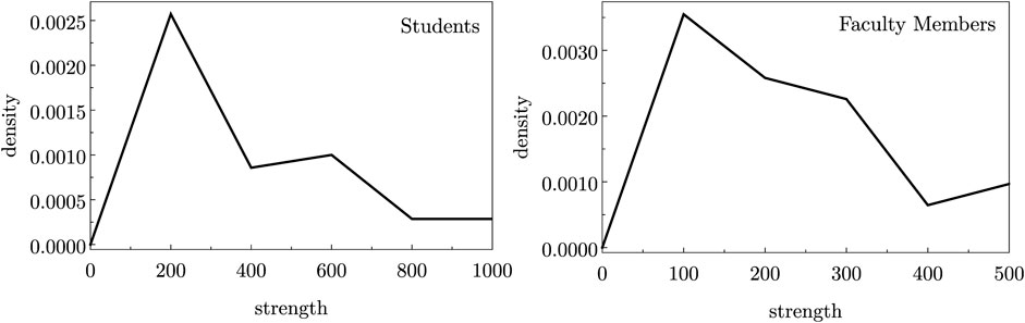
Figure 2. Histogram for the distribution of the vertices’ strengths $d_i={\sum }_{j=1}^n{\omega }_{ij}$. The non uniformity of this distribution, for both the groups investigated, reveals that the data are highly imbalanced.

The first outcome of the HodgeRank is the global ranking $\tilde{s}$, that associates a global score ${\tilde{s}}_i$ to the word i, where i ranges from 1 to n, where n is the number of words of the specific social group. Tables 3, 4 show the global rankings for the two groups investigated (students and faculty). In those tables, we also show, for the sake of comparison, the rankings obtained if we had used the individual binary comparison, or the individual logarithm of the score ratios, introduced at the beginning of Section 2.2.2, instead of the usual individual score differences $Y_{ij}^{\alpha }=r_j^{\alpha }-r_i^{\alpha }$. All three choices give essentially the same results, with just some slight changes in the ordering among words very closely ranked (and not at the top of the rankings). We will consider, for the rest of our analysis, only the global ranking obtained by using the individual score differences.

Table 3

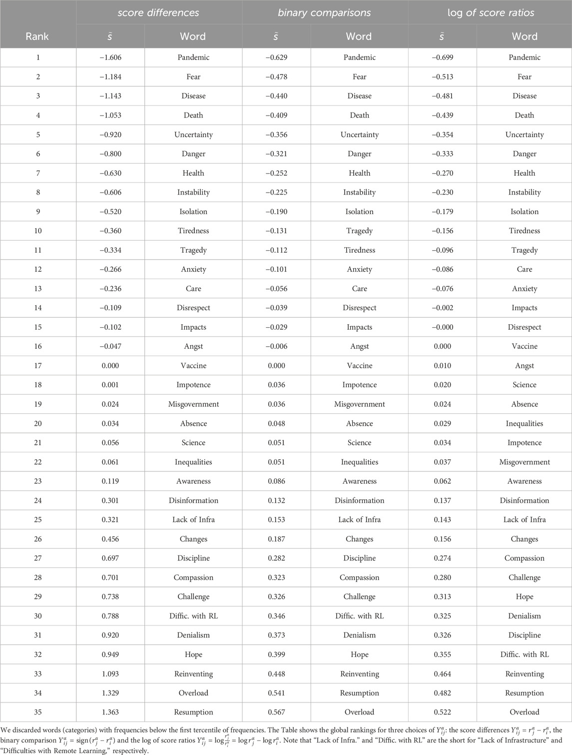
Table 3. Global ranking generated by the inducing word “COVID-19” for a group of students from Brazilian high education institutions.

Table 4

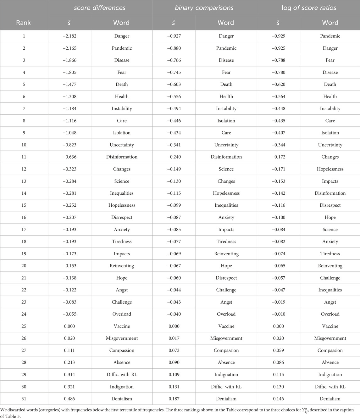
Table 4. Global ranking generated by the inducing word “COVID-19” for a group of faculty members from Brazilian higher education institutions.

The global scores within each social group define the gradient flow Y_g, whose matrix elements ${\left(Y_g\right)}_{ij}=a_{ij}\left({\tilde{s}}_j-{\tilde{s}}_i\right)$ give the (global) relative importance between the pair of words i and j in the group. Recall that a_ij = 1 if there was at least one individual in the group that evoked the pair of words i and j, and it is zero otherwise. From the set of words V and the adjacency matrix a = [a_ij], i, j ∈ V, we construct the gradient pairwise comparisons graph G(V, E) by assigning the gradient flow ${\left(Y_g\right)}_{ij}$ to each edge {i, j} ∈ E. The graph G(V, E), with the gradient flow Y_g, is analogous to an electric circuit with nodes labelled by i = 1, …, n, with admittances a_ij between nodes i and j, and with an electric current ${\left(Y_g\right)}_{ij}$ flowing from node i to the node j. This analogy holds since the currents in an electric circuit must satisfy ${\left(Y_g\right)}_{ij}=a_{ij}\left({\tilde{s}}_j-{\tilde{s}}_i\right)$, where ${\tilde{s}}_i$ is the electric potential of the node i; this is precisely the main result from the HodgeRank technique [see (9)]. Figures 3, 4 show the pairwise comparison graphs for the two social groups (students and faculty). In these figures, both graphs are drawn in such a way that the position of the word i in the left-right direction indicates its global score ${\tilde{s}}_i$ (giving its ordering in the global ranking), whereas its position in the up-down direction indicates its frequency of evocation. The edges are coloured according to their weights. The gradient edge flows ${\left(Y_g\right)}_{ij}$ are not shown, but are straightforwardly inferred from these figures, since they are proportional to the horizontal distances between the corresponding nodes, and are always directed from the left to the right. Going from the left to the right the relative importance of the words decreases, and from the top to the bottom the frequencies decrease. In both graphs, the nodes (words) were labelled by numbers, according to their ordering in the resulting global ranking. In both these graphs we have indicated by dashed lines the median values for the score (vertical line) and the frequency (horizontal line). These dashed lines delimit four regions, which will be compared to the four cells in the double entry Table 1 in the next section. At this point, it is worth mentioning that the graph structure behind these four regions provides more information about the structure of the SRs than does the Vergés’ double-entry table.

Figure 3

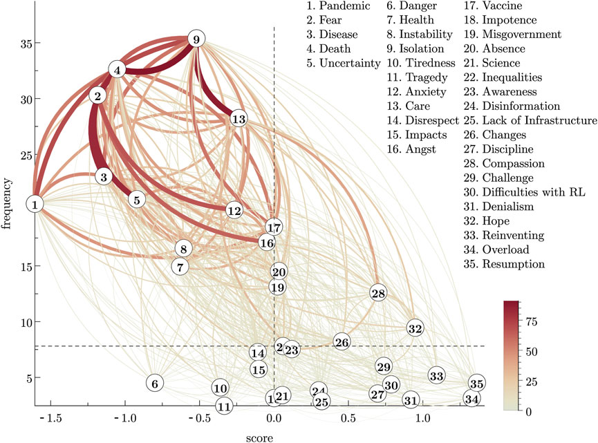
Figure 3. (Color online) Pairwise comparison graph for the social representation of “COVID-19” within a group of students from Brazilian higher education institutions, with a global ranking given in Table 3. The words are labelled by numbers giving their ordering in the global ranking. The scores ${\tilde{s}}_i$ increase in a scale from left to right, and the corresponding relative importance of the words decreases from the left to the right (the lower the score, the higher the relative importance). In this figure, ${\left(Y_g\right)}_{ij}$ is proportional to the horizontal distance between the words i and j, if the two words are linked (and is positive if ${\tilde{s}}_i<{\tilde{s}}_j$, negative if ${\tilde{s}}_i>{\tilde{s}}_j$, and zero if ${\tilde{s}}_i={\tilde{s}}_j$ or if the two words are not linked). The edges are drawn with thickness proportional to their weights, whose values are indicated by the colour scale at right. The position of each word in the top-bottom direction gives its frequency: the higher its position, the higher its frequency. The vertical dashed line indicates the median score $(\approx 0.001)$ and the horizontal dashed line indicates the median frequency $(\approx 7.81\%)$. The words located at the upper left “quadrant” are the “most salient ones,” and are the first candidates to form the central core of the SR.

Figure 4

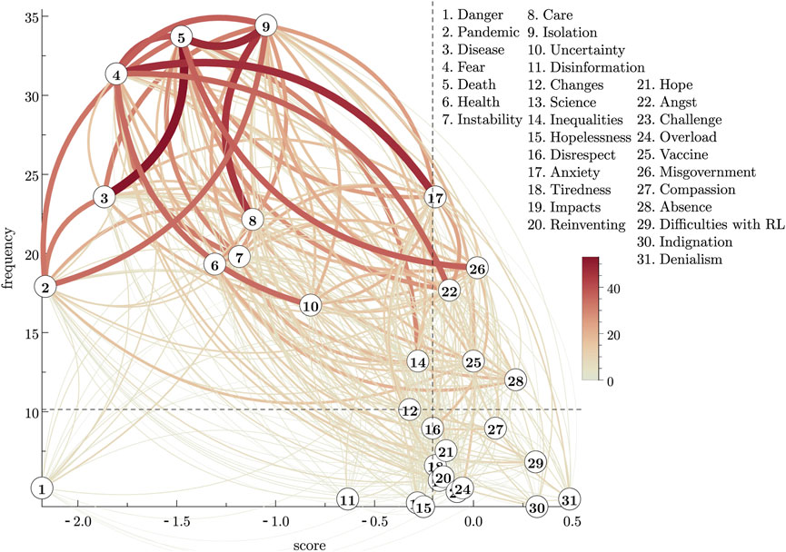
Figure 4. (Color online) Pairwise comparison graph analogous to that shown in Figure 3, with the same features described there, but now for the group of faculty members from Brazilian higher education institutions. The vertical dashed line indicates the median score $(\approx -0.207)$ and the horizontal dashed line indicates the median frequency $(\approx 10.14\%)$.

The other useful information provided by the HodgeRank concerns the ranking inconsistencies. Again, we recall that the ranking inconsistencies are not related to a weakness of the method. Instead, they are caused by inconsistent triangular or other cyclic rankings in the actual answers of the individuals within the social group. In general, the inconsistencies are related to instabilities in the structure of the SR, since they correspond to pairwise comparisons that were not “caught” by the optimal gradient flow. In Table 5 we show the inconsistencies computed according to Eq. 13. In this table, the value of P_g is related to the global consistency, i.e., the fraction of the norm of the observed flow Y that corresponds to the gradient flow Y_g. The higher the value of P_g, the greater the consistency of the global ranking achieved. On the other hand, the value of P_c is related to the local inconsistency, i.e., the fraction of the norm of the observed Y that corresponds to triangular inconsistencies. The other term, P_h, giving the cyclic (cycles of lengths $>3$), is straightforwardly given by 1 − P_g − P_c and is not shown in Table 5. We can observe that in both the groups the cyclic inconsistencies are negligible (i.e., P_h ≈ 0); therefore, the triangular inconsistencies are dominant, i.e., the local inconsistencies are responsible for essentially all the inconsistencies observed in the global rankings of the two groups. The reason behind the predominance of the local inconsistencies over the cyclic ones is the fact that the graphs G(V, E) for both groups show a very low sparsity, i.e., there are just a few numbers of edges missing, and, therefore, those graphs are “almost complete.”⁷

Table 5

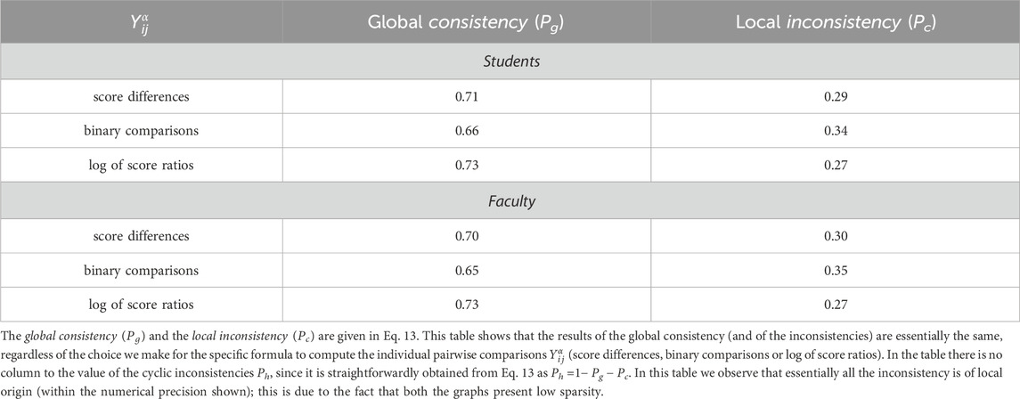
Table 5. Reliability of the rankings.

To help the visualization of the global rankings, in Figures 5, 6 we show matrix plots for three edge flows: the empirically observed pairwise comparisons Y, the gradient flow Y_g, determined by the global ranking $\tilde{s}$, and the difference between these two flows, R* = Y − Y_g. The difference R* allows one to identify the main sources of the inconsistencies in the global ranking, which are the pairs of observed comparisons that do not fit well to the resulting global ranking. Such edges are identified in the matrix plots of R* as being the darkest cells. In particular, for i < j a difference $R_{ij}^{*}<0$ (coloured in a bluish scale in those plots) means that the empirically measured importance of the word i over the word j (Y_ij) is less intense than that given by the global ranking $({\left(Y_g\right)}_{ij})$. Similarly, for i < j a difference $R_{ij}^{*}>0$ (cells colored in a reddish scale) means that the empirically measured importance of the word i over the word j (Y_ij) is more intense than that given by the global ranking $({\left(Y_g\right)}_{ij})$. In the next section, we will interpret the inconsistencies in terms of the instabilities in the SR structure.

Figure 5

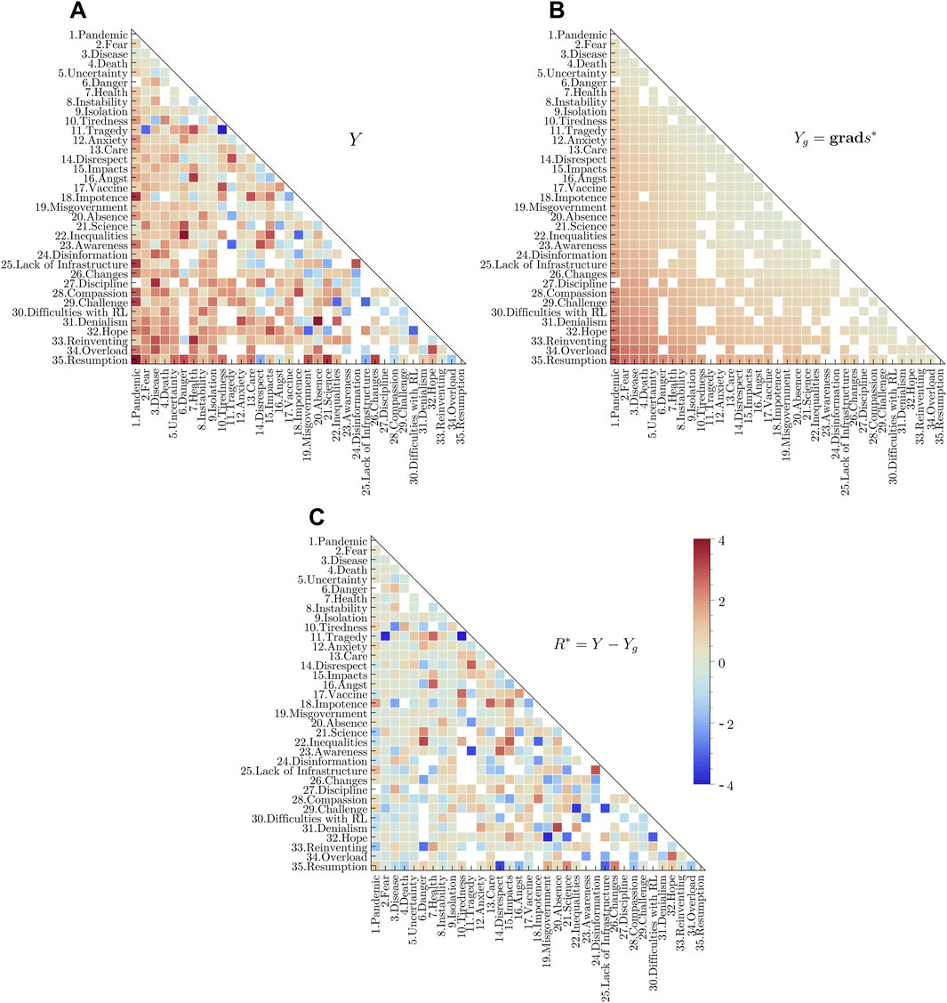
Figure 5. (Color online) Matrix plots representing (A) the edge flows Y (observed), (B) Y_g (defined from the global ranking), and (C) the difference between these two flows, R*= Y − Y_g, for the group of students. The words in the rows and columns are ordered according to their positions in the global ranking, as in the graph of Figure 3. In these plots, the blank cells correspond to the edges that are missing in the graph and, thus, illustrate the incompleteness of the pairwise comparison data. The colour scale indicates the values of the edge flows: Y_ij >0 if i < j, and vice versa, where i labels the rows and j the columns in these (skew-symmetric) matrices.

Figure 6

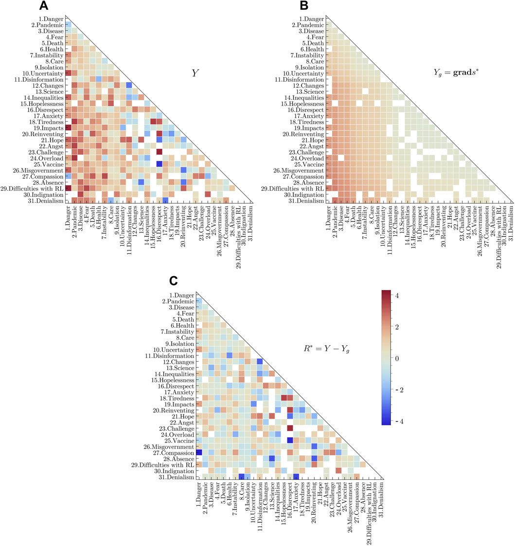
Figure 6. (Color online) Matrix plots representing (A) the edge flows Y (observed), (B) Y_g (defined from the global ranking), and (C) the difference between these two flows, R*= Y − Y_g, for the group of the faculty members. These matrix plots are built and interpreted in the same way as described in the caption of Figure 5.

We present also another useful way to visualize the instabilities in the structure of the SR: we will identify, in the gradient pairwise comparison graph (Figures 3, 4), the edges showing the greatest differences between the empirical and the gradient flows. These edges are those showing the greatest absolute values for R* = Y − Y_g and are identified in Figures 7, 8, for the two social groups studied. If, for a given pair i < j, the flow difference is positive (reddish scale in those figures), the relative importance ${\left(Y_g\right)}_{ij}$ of the pair in the global ranking is underestimated in comparison to the empirical values Y_ij. If, on the other hand, for i < j, that difference is negative (bluish scale), then the global ranking overestimate the relative importance of the corresponding pair of words in comparison to the empirical value. These situations have the potential to induce alterations in the SR structure over time, especially if both words in the pair have a high frequency, as we will discuss in the next section.

Figure 7

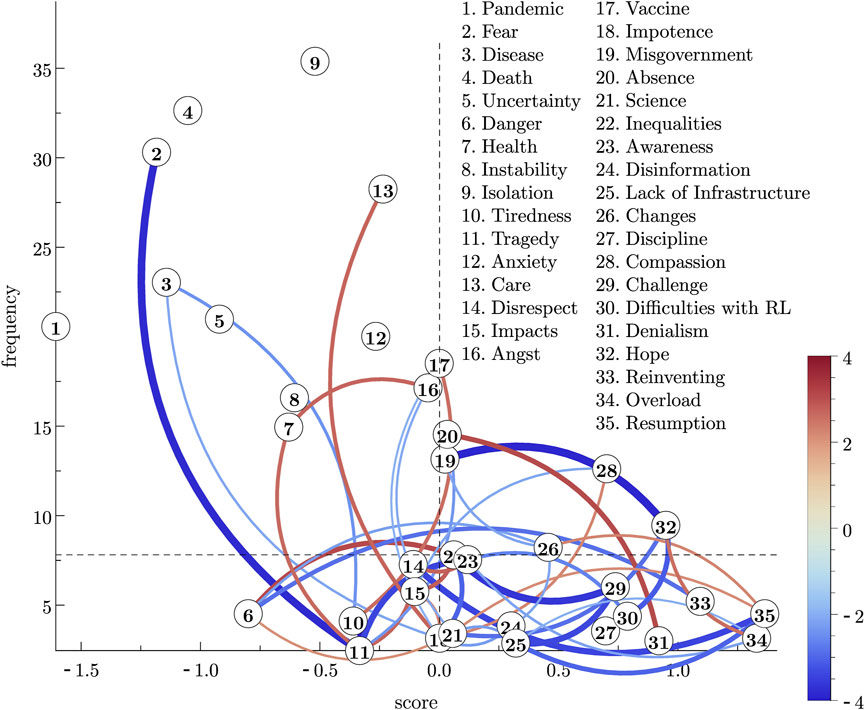
Figure 7. (Color online) The graph of Figure 3, concerning the group of students, in which we show only the edges with major differences between the observed (Y) and the gradient edge flow (Y_g). These edges are the major sources of inconsistencies in the global ranking. In this figure, we have shown only the edges with an edge flow difference $\left|R^{*}\right|=\left|Y-Y_g\right|>2$.

Figure 8

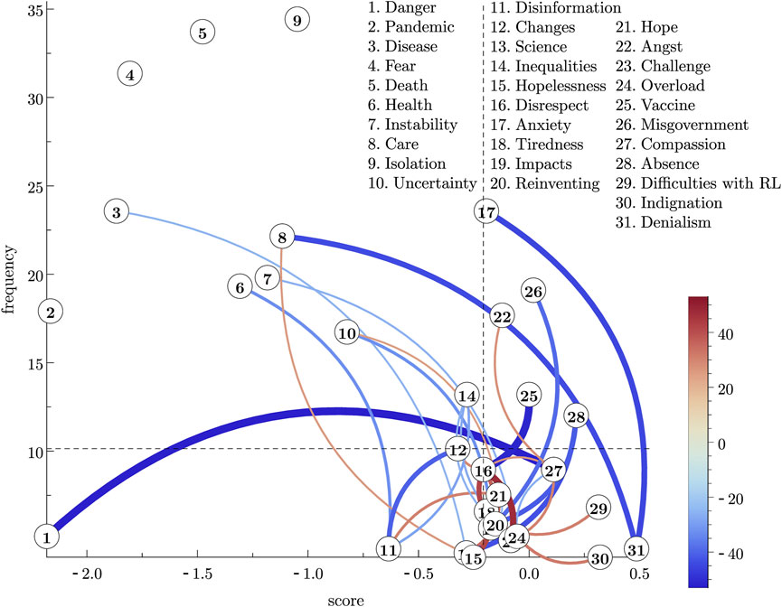
Figure 8. (Color online) The graph of Figure 4, concerning the group of faculty members, built in the same way as the graph in Figure 7, with the same cut-off in R*.

3.2 Discussion of the results

We start by discussing the structure of the global rankings in the two groups, with the aid of the graphs in Figures 3, 4. From the students’ graph (Figure 3) we can observe a “most salient” group of words in the top left region of the graph. These are the words best ranked and with the highest frequencies and are the first natural candidates to form the central core of the social representation. We have drawn the two dashed lines indicating the median values of the scores and the frequency, just to delimit 4 regions of reference. By using these reference thresholds, we may consider these first candidates to the central core as being the words ranked in the positions 1,2,3,4,5,7,8,9,12,13,16 and 17, which are shown in Table 6.

Table 6

Table 6. First candidates to the central core of the social representation of “COVID-19” in a group of students from Brazilian higher education institutions. This set will be refined by using a stability criterion, and the underlined word (“Angst”) will be removed; the remaining words will form the set of “best” candidates.

However, one criterion to be part of the central core is that the set of elements in the central core be stable [16]. In the context of the HodgeRank, we will associate the stability of a word to its frequency and the consistency of their connections to the other words. More precisely, we will say that a word i is stable if it is a high-frequency word whose empirical edge flows Y_ij linking it to other high-frequency words j are close to the corresponding gradient flows ${\left(Y_g\right)}_{ij}$. We will not set rigid boundaries for the notions of “high frequency” or “closedness” to the gradient flows, since we are using the HodgeRank as an exploratory tool to identify the “best” candidates to the central core. These candidates should be ultimately submitted to hypotheses tests to assess their centrality [17, 6]; such further tests are out of the scope of the present work. We claim that we can already get relevant information about the structure and the dynamics of the SR by simply analysing the outcomes of HodgeRank, even if such information is still exploratory. Below we discuss the use of the stability criterion just stated to further refine the set of candidates to the central core presented in Table 6.

Observing the graph of the differences R* = Y − Y_g in Figure 7 we see that, among the first candidates to the central core, some few pairs present significative inconsistencies between high-frequency words. The first significative inconsistency appears in the pair 7–16 (“Health”—“Angst”). The reddish colour of that connection means that the global ranking subestimates the empirical one; that inconsistency tends to take the words in the pair far away from each other. If such tendency were consolidated in future observations of the group, the word 16 (“Angst”) could move outwards the central core; whereas the word “Health” would move inwards the central core region, thus consolidating its position as a central element; for this reason, we may discard the word 16 (“Angst”) as a good candidate to the central core, and may retain “Health” as a good candidate. The other words in Table 6 do not participate in largely unstable connections, since the remaining large inconsistencies in which these words participate involve only low-frequency words. Thus, we may consider all the words in this table, except the underlined word (“Angst”) as forming the set of the “best” candidates to the central core.

The above reasoning based on the stability criterion was used to refine the set of the “first” to the set of the “best” candidates to the central core. We also may use the instabilities of words (not necessarily belonging to the candidates to the central core) to explore some conjectures about the dynamics of the SR structure. The dynamics refers to potential moves of elements within the dual system (i.e., moves from the central to the peripheral system, and vice versa). From Figure 7, the largest inconsistency in the subsector of the peripheral system formed by high frequency and poorly ranked words (the upper right region of the graph) is observed in the pair 19–32 (“Misgovernment”—“Hope”). The bluish colour in that link means that the global ranking overestimates the pairwise comparison between these two words; therefore, the actual comparison is less intense. If such behaviour were to be consolidated in future observations, it would tend to approximate these two words in the ranking.⁸ In such a case, the word 19 (“Misgovernment”) would tend to move inwards the peripheral system, thus potentially not being a source for changes in the SR structure. The other large inconsistencies shown in Figure 7 involve at least one low-frequency word and is not very likely that they may cause changes in the SR structure. Such a statement can be verified by observing the matrix plot in Figure 5, which shows all the sources of inconsistencies, together with the global ranking graph in Figure 3, from which we can read the words’ frequencies. Concluding our exploratory analysis with HodgeRank regarding the group of students, we may conjecture that the dual system with the “best” candidates to the central core shown in Table 6 (with “Angst” excluded), and the remaining ones forming the peripheral system, form a structure which is robust against changes in the near future. Comparing the best candidates shown in Table 6 with the upper left cell in the double entry Table 1 of Section 2.1, we observe that the criteria we used together with the HodgeRank to identify the best candidates include all those candidates to the central core present in Table 1, and adds other three candidates (“Vaccine,” “Health,” and “Anxiety”).

Now we will proceed by discussing the HodgeRank results for the group of faculty members. Similarly to what we have done for the group of students, we will identify the set of first candidates to the central core, by observing the words in the upper left region in the graph of Figure 4. These words are given in Table 7. It is worth noticing that the best-ranked word (“Danger”) is not included in this set, since it has a very low frequency and, thus, does not share a high consensus within the group. No word in this table is significantly unstable, according to the stability criterion we stated above; thus, all the words in Table 7 belong to the set of “best” candidates to the central core.

Table 7

Table 7. First candidates to the central core of the social representation of “COVID-19” in a group of faculty members from Brazilian higher education institutions. This set will coincide with the set of “best” candidates since no word in this set shows large instability.

In regards to the dynamics of this SR representation, we observe in Figure 8 that there are no large inconsistencies involving pairs of high-frequency words. The main inconsistencies shown in that figure always involve at least one low-frequency word. Therefore, the high-frequency words are highly stable. The matrix plot in Figure 6, analysed together with the graph in Figure 4, corroborates such a statement. From this feature, we may conjecture that the faculty’s SR structure identified by HodgeRank for the faculty members group, in which the words in Table 7 are the best candidates to the central core, and the remaining ones form the peripheral system, is very robust against changes in the near future. Comparing with the results from Table 2, in Section 2.1, we observe that the candidates for the central core essentially coincide: in the set identified by the HodgeRank an additional word (“Inequalities”) was included (but it is the less salient among all the best candidates).

In the two social groups studied here, we can observe that the inconsistencies tend to be more significant in the peripheral system, as claimed by the central core theory [15, 16]. The upper-left regions of the matrix plots shown in Figures 5, 6 show little differences between the flows in the ranked solution and those empirically observed; the exceptions regard in general inconsistent flows linking a high-frequency word to a low frequency one. When an inconsistency is observed in a link between two high-frequency words, as in the case of the pair“Health”—“Angst” in the students’ group, this was interpreted as a source of instability. The instability was interpreted as a negative feature for a word to be considered as a good candidate for the central system, as well as a possible source driving the dynamics of the SR, i.e., the potential moves of elements within the dual system.

4 Conclusion

In this work, we presented the basics of the HodgeRank technique and proposed its use to explore the structure of social representations. By using as input the same kind of data collected for the classical methodology of hierarchical word associations, the HodgeRank technique proved to be a powerful method to extract exploratory information about the structure of the social representation. In this context, it is more effective than the usual Vergés’ double entry table, in the sense that, besides identifying a set of best candidates to form the central core of the representation, the outcomes of the HR technique also reveal a graph structure among the elements (words, or categories) of the representation. Such a structure is analogous to an electric circuit, in which each word is associated with a score (the “electric potential”), and between two linked words there is a flow (the “electric current”) determined by the score differences between these words. The analogous “electric circuit” is associated with an optimal global ranking of the words (or categories), which extends to the whole group the relative importance that the group of individuals assigns to a pair of words. This graph is also a weighted graph, and its structure is richer than (and includes) that revealed by similarity graphs.

The global ranking, being a solution for an optimisation problem, does not fit exactly all the observed pairwise comparisons in the group. Such differences give rise to inconsistencies in the ranking, which can be of two different kinds: local and cyclic. In the two groups studied, the pairwise comparison graphs presented low sparsities, and, therefore, the inconsistencies were essentially local, i.e., all the inconsistencies were essentially reduced to triangular ones. On the other hand, if we had observed a disconnected pairwise comparison graph, or a high global inconsistency in the ranking within a given group this would suggest a lack of consensus within the group and would raise questions about the methodology of the group delimitation. In the two groups studied here, we obtained highly connected graphs, and the global inconsistencies were not high (about 30%).

From the graph representing the optimal gradient flow (associated with the global ranking solution, analogous to an electric circuit) we identified a set of first candidates to the central core as those words being the best ranked and most consensual within the group. After, we refined this set by requiring that the best candidates to the central core should also be stable, in the sense that they should be high-frequency words having highly consistent links to other high-frequency words. Besides serving to characterise the best candidates for the central core, the analysis of stability also served to explore the potential dynamics of the SR: unstable linkings tending to cause moves to and from the two systems (central and peripheral system) were considered as possible sources for changes in the SR structure along the time. Inconsistencies in the peripheral system appear as inconsistencies between the empirical data and the global ranking, and these may be drivers of potential changes in the SR. Figures 7, 8 are “photographies” of the two systems (central core and peripheral system) that identifies the more likely potential drivers of future changes in the SR; these changes may remain in the periphery or they cause elements of the periphery to move to the central core [16], or vice versa.

We illustrated the application of the HodgeRank technique to explore the structure and the potential dynamics of the social representations of the inducing term “COVID-19” within two social groups from high education institutions in Brazil, namely, a group formed by students (including undergraduate and graduate students), and the other formed by faculty members. For the two groups, our results concerning the identification of the best candidates for the central core essentially corroborated the results obtained from the Vergés double-entry table in Section 2.1. Besides corroborating those results, the HodgeRank also revealed a structure between the words, and with a criterion of stability based on the frequency of evocation and the ranking inconsistencies, we were able to better characterise the candidates to the central core, as well as to raise conjectures about the possible dynamics of the structure within the two groups. In both groups, we observed a high robustness against changes in the SR structure in a brief period of time. The observed robustness against such changes was more evident in the group of faculty members.

We finalize by stressing some of the main advantages of using the HodgeRank when exploring the structure of a social representation. Despite the mathematical technicalities behind the method, it i) is simple to apply, with a single data collection, and by running a simple algorithm, ii) reveals a structure among the elements of the representation, in the form of a weighted graph that is analogous to an electric circuit, iii) provides means to characterise the stability of the elements of the representation, and iv) allows one to raise conjectures about the dynamics of the social representation. Due to all these features, we claim that HodgeRank is a quantitative tool that can be used to make powerful exploratory investigations in the research field of social representations.

Data availability statement

The raw data supporting the conclusion of this article will be made available by the authors, without undue reservation.

Ethics statement

The studies involving humans were approved by the Comitê de Ética em Pesquisa da Universidade Estadual de Ponta Grossa (CEP-UEPG). The studies were conducted in accordance with the local legislation and institutional requirements. The participants provided their written informed consent to participate in this study.

Author contributions

LO: Conceptualization, Formal Analysis, Investigation, Methodology, Software, Writing–original draft, Writing–review and editing. JL: Conceptualization, Formal Analysis, Investigation, Methodology, Project administration, Software, Supervision, Writing–original draft, Writing–review and editing. MC: Conceptualization, Formal Analysis, Investigation, Software, Supervision, Writing–original draft, Writing–review and editing. AP: Data curation, Investigation, Writing–review and editing. DJ: Data curation, Investigation, Writing–review and editing. CC: Data curation, Investigation, Writing–review and editing.

Funding

The author(s) declare that financial support was received for the research, authorship, and/or publication of this article. This work is supported by the Brazilian agencies CNPq (Grants 122384/2018-0 and 164201/2019-0) and CAPES (Grant 88887.927927/2023-00).

Acknowledgments

LO thanks the Brazilian agencies CNPq and CAPES for full support. The authors thank all the referees, whose comments and suggestions helped to improve the quality of the paper.

Conflict of interest

The authors declare that the research was conducted in the absence of any commercial or financial relationships that could be construed as a potential conflict of interest.

The author(s) declared that they were an editorial board member of Frontiers, at the time of submission. This had no impact on the peer review process and the final decision.

Publisher’s note

All claims expressed in this article are solely those of the authors and do not necessarily represent those of their affiliated organizations, or those of the publisher, the editors and the reviewers. Any product that may be evaluated in this article, or claim that may be made by its manufacturer, is not guaranteed or endorsed by the publisher.

Footnotes

¹In our study, the first tercentile corresponds to a frequency of 2.19% (3.53%) for the group of students (faculty). We dropped out 33.96% (34.04%) of the words cited by the students’ (faculty) social group. We will use these same cuts in our reanalysis of the data with the HodgeRank method.

²The full set of words/categories is identified only a posteriori, after the categorisation procedure, described in Section 2.1.

³The above choice of aggregating the individual pairwise comparisons by the average over the individuals is suitable to compare pairwise comparison graphs of different groups when the set of objects ranked are the same (same V).

⁴We use the norm induced by the inner product.

⁵In our application to social representations, the HodgeRank algorithm takes as input a matrix with lines and columns representing, respectively, the voters and the cited words. In the examples studied, such a matrix has the dimensions 729 × 53 and 424 × 47 for, respectively, the students’ and faculty members’ group. The HodgeRank procedure took around 30s (10s) for the computations of the students’ (faculty members’) dataset (this computation time is shown in the third output of our code). It is worth noting that our algorithm was implemented in the Wolfram Mathematica Language and executed on a laptop equipped with a Intel^® Core™ i5-10500H processor and with 16 GB memory.

⁶A cycle in a graph is a closed, nonself crossing path formed by a sequence of vertices of the graph, such that there is an edge between any two successive vertices in this sequence.

⁷Recall that in a complete graph the cyclic inconsistencies vanish, with all the inconsistencies arising from the local (triangular) ones.

⁸An intuitive way to interpret the colours in the inconsistent links shown in Figures 7, 8 is in the following way. The reddish colours tend to put the words in the pair far away from each other in the ranking, whereas the bluish colours tend to approximate the two words.

References

1. Moscovici S. Psychoanalysis, its image and its public. Cambridge: Polity Press (2008).

Google Scholar

2. Moscovici S. Attitudes and opinions. Annu Rev Psychol (1963) 14:231–60. PMID: 13936119. doi:10.1146/annurev.ps.14.020163.001311

PubMed Abstract | CrossRef Full Text | Google Scholar

3. Moskovici S. The history and actuality of social representations. Cambridge University Press (1998).

Google Scholar

4. Wagner W, Duveen G, Farr R, Jovchelovitch S, Lorenzi-Cioldi F, Marková I, et al. Theory and method of social representations. Asian J Soc Psychol (1999) 2:95–125. doi:10.1111/1467-839X.00028

CrossRef Full Text | Google Scholar

5. Rateau P, Moliner P, Guimelli C, Abric JC. Social representation theory, In: Handbook of theories of social psychology. SAGE Publications Ltd (2012). p. 477–97. doi:10.4135/9781446249222

CrossRef Full Text | Google Scholar

6. Piermattéo A, Tavani JL, Monaco GL. Improving the study of social representations through word associations: Validation of semantic contextualization. Field Methods (2018) 30:329–44. doi:10.1177/1525822X18781766

CrossRef Full Text | Google Scholar

7. Howarth C. A social representation is not a quiet thing: exploring the critical potential of social representations theory. Br J Soc Psychol (2006) 45:65–86. doi:10.1348/014466605X43777

PubMed Abstract | CrossRef Full Text | Google Scholar

8. Höijer B. Social representations theory: a new theory for media research. Nordicom Rev (2011) 32:3–16. doi:10.1515/nor-2017-0109

CrossRef Full Text | Google Scholar

9. Vuillot C, Mathevet R, Sirami C. Comparing social representations of the landscape: a methodology. Ecol Soc (2020) 25:28. doi:10.5751/ES-11636-250228

CrossRef Full Text | Google Scholar

10. Feitosa EAL, Ferreira Júnior A, Techio EM. Sistema de Representações Sociais em sentenças jurídicas de feminicídio na Bahia nos anos de 2020 e 2021. Revista de Psicología (2024) 42:466–502. doi:10.18800/psico.202401.016

CrossRef Full Text | Google Scholar

11. Lampert DA, Porro S. Emotions and interests in social representations about the environmental problem of arsenic in water in tandil (buenos aires, Argentina). Front Education (2023) 8. doi:10.3389/feduc.2023.1305788

CrossRef Full Text | Google Scholar

12. Higuita-Gutiérrez LF, Estrada-Mesa DA, Cardona-Arias JA. Social representations of cancer in patients from medellín, Colombia: a qualitative study. Front Sociol (2023) 8:1257776. doi:10.3389/fsoc.2023.1257776

PubMed Abstract | CrossRef Full Text | Google Scholar

13. Faurie I, Harroch E, Scotto d’Apollonia C, Corte S, Arcari C, Mohara C, et al. Impact of therapeutic education on the evolution of social representations of medication in patients with Parkinson’s disease: a quantitative and qualitative study (etpark remed). Revue Neurologique (2023) 179:1086–94. doi:10.1016/j.neurol.2023.03.026

PubMed Abstract | CrossRef Full Text | Google Scholar

14. Wallace R, Batel S. Representing personal and common futures: insights and new connections between the theory of social representations and the pragmatic sociology of engagements. J Theor Soc Behav n/a (2023) 54:65–85. doi:10.1111/jtsb.12398

CrossRef Full Text | Google Scholar

15. Abric JC. Central system, peripheral system: their functions and roles in the dynamics of social representations. Pap Soc Representations (1993) 2:75–8.

Google Scholar

16. Moliner P, Abric JC. Central core theory. In: The cambridge handbook of social representations. Cambridge University Press (2015). p. 83–95. doi:10.1017/CBO9781107323650.009

CrossRef Full Text | Google Scholar

17. Lo MG, Piermattéo A, Rateau P, Tavani JL. Methods for studying the structure of social representations: a critical review and agenda for future research. J Theor Soc Behav (2017) 47:306–31. doi:10.1111/jtsb.12124

CrossRef Full Text | Google Scholar

18. Abric J. Jeux, conflits et représentations sociales (Éditeur inconnu) (1976).

Google Scholar

19. Dany L, Urdapilleta I, Lo Monaco G. Free associations and social representations: some reflections on rank-frequency and importance-frequency methods. Qual Quantity (2015) 49:489–507. doi:10.1007/s11135-014-0005-z

CrossRef Full Text | Google Scholar

20. Vergés P. Approche du noyau central: Propriétés quantitatives et structurales. ZX (1994) 233–53.

Google Scholar

21. Pereira AL, Lunardi JT, Calçada M, Viviane A B. Hodgerank as a quantitative tool in social representations theory. J Phys Conf Ser (IOP Publishing) (2019) 1391:012114. doi:10.1088/1742-6596/1391/1/012114

CrossRef Full Text | Google Scholar

22. Lim LH. Hodge laplacians on graphs. Siam Rev (2020) 62:685–715. doi:10.1137/18m1223101

CrossRef Full Text | Google Scholar

23. Jiang X, Lim LH, Yao Y, Ye Y. Statistical ranking and combinatorial hodge theory. Math Programming (2011) 127:203–44. doi:10.1007/s10107-010-0419-x

CrossRef Full Text | Google Scholar

24. Xu Q, Huang Q, Jiang T, Yan B, Lin W, Yao Y. Hodgerank on random graphs for subjective video quality assessment. IEEE Trans Multimedia (2012) 14:844–57. doi:10.1109/tmm.2012.2190924

CrossRef Full Text | Google Scholar

25. Wei RKJ, Wee J, Laurent VE, Xia K. Hodge theory-based biomolecular data analysis. Scientific Rep (2022) 12:9699. doi:10.1038/s41598-022-12877-z

CrossRef Full Text | Google Scholar

26. Schenck H, Sowers R, Song R. Trading networks and hodge theory. J Phys Commun (2021) 5:015018. doi:10.1088/2399-6528/abd1c2

CrossRef Full Text | Google Scholar

27. University P. About wordnet (2010).

Google Scholar

28. Mikolov T, Sutskever I, Chen K, Corrado G, Dean J. Distributed representations of words and phrases and their compositionality. arXiv e-prints (2013). arXiv:1310.4546. doi:10.48550/arXiv.1310.4546

CrossRef Full Text | Google Scholar

29. Schaub MT, Benson AR, Horn P, Lippner G, Jadbabaie A. Random walks on simplicial complexes and the normalized hodge 1-laplacian. SIAM Rev (2020) 62:353–91. doi:10.1137/18m1201019

CrossRef Full Text | Google Scholar

Appendix A: An algorithm to implement the HodgeRank technique

In Table 8 we present a pseudocode with the steps described in Section 2.2, needed to run the HodgeRank technique in order to obtain an optimal global ranking and the ranking inconsistencies. The input data are the individual hierarchical word associations, after the categorisation procedure. The graphs and the matrix plots shown in the main text were built with the aid of the Wolfram Language^© resources.

TABLE 8

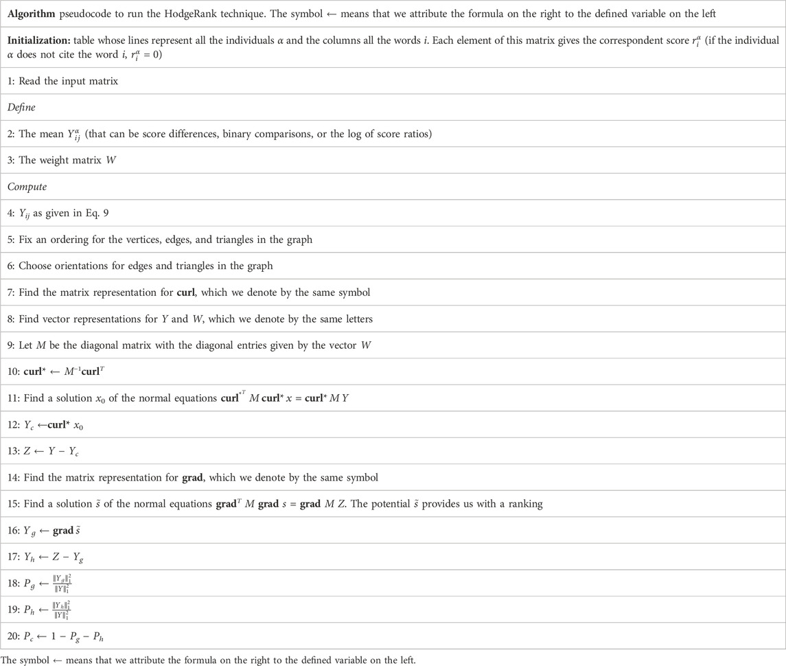
TABLE 8. Pseudocode based on the method described before.