Data-driven RANS closures for improving mean field calculation of separated flows

1 Introduction

Owing to the inherently chaotic characteristics of turbulence, its numerical prediction turns out to be highly challenging. The Reynolds-averaged Navier-Stokes (RANS) simulation serves as a standard technique for predicting turbulence, establishing itself as the primary tool employed in the majority of industrial computations [1]. Despite the superior accuracy provided by the Direct Numerical Simulation (DNS) and Large-Eddy Simulation (LES), the RANS method proves more resource-efficient [2]. The closure terms within the RANS equations employ various modeling methods, which can be classified into three categories. The first and most basic category encompasses the mixing length-based model [3], colloquially referred to as the zero equation model. Despite its computational cost-efficiency, this model proves apt primarily for simpler flows and lacks sufficient accuracy for more intricate scenarios. The second category includes eddy viscosity-based models, incorporating one-equation models such as the Spalart-Allmaras (SA) model [4], and two-equation models like the k-ϵ, k-ω models, k-ω SST model. These models hinge on the assumption of eddy viscosity to establish a linear association between the Reynolds stress and strain rate tensor [5]. Although this approach amplifies generality and robustness, it manifests notable constraints in complex flows, including flow separation and reattachment [6, 7]. The third category comprises the Reynolds Stress Model (RSM), which formulates transport equations for each component of the Reynolds stress, frequently termed as the seven-equation model [8]. Although RSM offers higher accuracy, it is computationally demanding and performs poorly in flows with substantial curvature.

Traditionally, turbulence modeling has evolved using a combination of intuition, asymptotic theory and empiricism, where turbulence closure models were formulated by physical arguments [9]. The coefficients of the closure terms were determined by calibrating experimental or DNS data, highlighting the source of errors in RANS models. However, the advent of artificial intelligence has facilitated the application of Machine Learning (ML) techniques to establish mapping relationships between closure terms and flow field data. Data-driven methodologies have been subsequently employed for closure in the RANS model, transcending simple physical relationships [10]. Utilizing supervised learning, a mapping can be constructed between flow field features and high-fidelity data, theoretically mitigating the error from closure terms to a markedly reduced level [11]. This accomplishment, though challenging to attain in traditional turbulence modeling, becomes feasible with data-driven turbulence modeling. Within the framework of data-driven closure turbulence models, various methods have been proposed to accommodate diverse RANS models. While some researchers have displayed interest in RSM [12, 13], the majority of investigations have revolved around the Linear Eddy Viscosity Model (LEVM).

Zhu et al. [14] implemented a neural network to construct a mapping between the eddy viscosity and the mean flow field derived from the Spalart-Allmaras (SA) model, with two distinct coupling modes compared by Liu et al. [15]. The coupling mode refers to the approach through which the predicted values are integrated into the RANS equation. Maulik et al. [16] devised a mapping between steady-state turbulent eddy viscosities and initial conditions. Such surrogate models, electing learning targets from the RANS mean field, cannot surpass the original RANS models in terms of accuracy. Despite this, they afford a reduction in computational cost by obviating the need to solve the partial differential equation. A series of augmented models were developed [17–20] by selecting learning targets from high-fidelity fields or by targeting the differences between high-fidelity fields and SA mean fields. These augmented models generated improved results while retaining the advantages of the SA model.

Ling and Templeton [21] investigated the uncertainty region of the k-ϵ model using several machine learning algorithms, and successfully procured the Reynolds stress anisotropy tensor from high-fidelity data, leveraging both random forests [22] and neural networks [23]. They proposed the Tensor Basis Neural Networks (TBNN) with higher prediction accuracy, and improved the velocity fields by integrating the Reynolds stress anisotropy tensor into the converged k-ϵ fields. Significantly, the TBNN has been extensively adopted and refined by numerous researchers investigating data-driven turbulence models, consistently producing commendable predictions [24, 25]. Furthermore, Wang et al. [26] introduced a Physics-Informed Machine Learning (PIML) approach that considered the invariance of the framework. They targeted the discrepancies in the Reynolds stress between DNS and the Launder-Sharma k-ϵ models in the case of a periodic hill, employing random forests to forecast these discrepancies. To further enhance the invariance of the PIML framework, Wu et al. [27] developed a minimal integrity basis comprising turbulent quantities like velocity, pressure, and turbulent kinetic energy. The first invariants of these invariant bases were utilized as inputs for the ML model, enabling successful prediction of discrepancies in Reynolds stress. Beyond these studies, additional research has been undertaken based on the k-ϵ model. Chang et al. [28], Xu et al. [29] established surrogate models, demonstrating that the flow features based on the first order spatial derivative of the velocity field are both necessary and sufficient. Heyse et al. [30] provided uncertainty estimates for eddy viscosity models. Moreover, Zhang et al. [31] utilized deep learning to replace the source term in the ϵ equation and introduced a data correction method named “coordinate” technology. More recently, apart from the ML methods mentioned above, other techniques such as the discrete adjoint method [32], symbolic regression method [33], and field inversion machine learning (FIML) method [34] have likewise exhibited promising results within this domain.

In addition to the studies based on k-ϵ model, the k-ω SST model has also been considered as a research template. Liu et al. [35] proposed an iterative framework where the mean flow features and labels used for training are sourced from DNS data. Contrary to the prevalent one-loop frameworks, this methodology engages a machine learning model to predict the Reynolds stress at each time step, thus enhancing performance in relation to the k-ω SST model. Subsequent research by Liu et al. [36] further enhanced the model’s generalization performance by adopting a bounded normalization method. Similar to TBNN, Kaandorp and Dwight [37] propose a Tensor-Based Random Forest (TBRF) algorithm, which, notably, is more straightforward to implement and train. Shifting the focus away from Reynolds stress or constitutive components, Wu et al. [38] exploited an Artificial Neural Network (ANN) to learn the intermittency factor γ in Mentor’s SST-γ model. While many researchers consider the machine learning methods as black boxes, some aim to demonstrate algebraic relationships. Zhao et al. [39] obtained an explicit algebraic model using the gene expression programming (GEP) method. Frey Marioni et al. [40] utilized high-fidelity data and ANN to generate alternative Reynolds stress anisotropy formulations to replace the standard Boussinesq approximation. In a novel approach, Schmelzer et al. [41] introduced the Symbolic Regression method, termed as Sparse Regression of Turbulent Stress Anisotropy (SpaRTA), to deduce algebraic stress models for the closure term. These models, formulated as tensor polynomials, were inferred from high-fidelity data and allowed for a cost-effective correction of the k-ω SST model. Additionally, the works of Huijing et al. [42], Zhang et al. [43], Cherroud et al. [44] have been instrumental in the further promotion and enhancement of SpaRTA.

Studies focusing on eddy viscosity models hold practical significance when exploring various RANS models as templates for data-driven turbulence modeling. A key concern revolves around effectively integrating the predicted values from ML into the CFD process. To enhance the prediction accuracy of eddy viscosity models, researchers often choose to optimize inaccurately fitted closure terms. An important discovery by Wu et al. [45] revealed that directly substituting the RANS closure term with the DNS Reynolds stress led to an ill-conditioned equation. This issue was effectively resolved by decomposing the Reynolds stress into linear and nonlinear parts. The widely adopted treatment involves integrating the linear part into the viscous term of the Navier-Stokes equation, while utilizing the nonlinear term as a source term [27]. Building upon this basis, McConkey et al. [46] imposed a non-negative constraint on the linear part. More challenging scenarios were explored by Guo et al. [47, 48], who constructed the linear and nonlinear terms solely from high-fidelity Reynolds stresses, while disregarding the high-fidelity velocity information. This concept has also been embraced by Volpiani et al. [49], Berrone and Oberto [50], among others, with several studies demonstrating the improved prediction accuracy resulting from this approach.

However, several challenges arise with this approach. To improve the prediction accuracy of both the linear and nonlinear terms, researchers often utilize an extensive set of input features. Incorporating input features based on a minimal integrity basis results in a complex structure for the ML model, which is further compounded when mean flow features are included. Such excessively intricate ML models not only present difficulties during training but also carry an increased risk of overfitting. In most cases, the prediction of linear and nonlinear terms is carried out independently, and subsequently, these terms undergo transformations to account for physical factors, leading to more intricate representations. However, in addition to the inherent stochastic nature of prediction errors, the reconstruction of both linear and nonlinear terms may introduce unexpected variations. These deviations can subsequently manifest in the reconstructed Reynolds stresses, resulting in discrepancies from the high-fidelity data, and such errors may propagate to other flow field quantities. Hence, we intend to advance this methodology by simplifying the inputs and outputs of the ML model, thereby reducing the number of inputs while ensuring invariance. Moreover, we aim to employ a straightforward expression for the output, thereby minimizing unnecessary errors during the reconstruction of the Reynolds stress.

This paper introduces a data-driven turbulence model that employs the k-ω SST model as the correction template. The k-ω SST model, although widely utilized, exhibits limitation in accurately predicting flow separation. The primary objective of our proposed model is to improve the performance of the k-ω SST model, particularly in complex flow scenarios. To achieve this, our model adopts the entire Reynolds stress as the learning target, derived from a high-fidelity dataset. During the training process, the Reynolds stress is decomposed into linear and nonlinear components, and two distinct neural networks are constructed to predict these components individually. The predicted values are reconstructed to form a predictive closure term that participates in the RANS calculation. Importantly, the nonlinear part, representing the residual portion generated during the Reynolds stress approximation, is predicted directly to avoid excessive transformations. This treatment aims to minimize the accumulation of random errors during the restructuring process, thereby improving the accuracy of the prediction results. Additionally, we employ a reduced amount of data during training to demonstrate the effectiveness of our approach with the least amount of high-fidelity data, thereby establishing the rationality of the data-driven model framework.

The present work is structured as follows: Section 2 elucidates the decomposition method of the closure term, delineates the prediction objectives for machine learning, and outlines the structure of the comprehensive data-driven model. Section 3 introduces the structure and input features of neural networks, and discusses the normalization methods for input features and labels. Section 4 exhibits the training and prediction results of the data-driven model. Detailed discussions on the closure term and velocity prediction in interpolation tests, in comparison with high-fidelity data, are provided. Finally, conclusions are given in Section 5.

2 Methodology

For incompressible flows, the steady-state Reynolds-averaged Navier-Stokes equations can be expressed as Eqs 1, 2.

$\nabla \cdot \mathit{U}=0,(1)$

$\nabla \cdot \left(\mathit{U}\mathit{U}\right)-\nabla \cdot \nu \left[\nabla \mathit{U}+{\left(\nabla \mathit{U}\right)}^{\text{T}}\right]=-\nabla p+\nabla \cdot \mathit{\tau },(2)$

where U is the mean flow velocity, ν is the molecular kinematic viscosity, p is the pressure normalized by the constant density of the fluid and $\mathit{\tau }=-\overline{{\mathit{u}}^{\prime }{\mathit{u}}^{\prime }}$ is the Reynolds stress tensor. Here, u′ corresponds to the fluctuating velocity, which is defined as the difference between the instantaneous velocity and the average velocity.

The unclosed term τ can be decomposed into isotropic and anisotropic parts. The commonly used LEVM posits that the anisotropic component is equivalent to the product of the eddy viscosity coefficient and the time-averaged strain rate, commonly referred to as the Boussinesq assumption. Mathematically, this can be expressed as

$\mathit{\tau }=\mathit{a}-\frac{2}{3}k\mathit{I}\approx 2{\nu }_t\mathit{S}-\frac{2}{3}k\mathit{I},(3)$

where a designates the anisotropic tensor, ν_t stands for the eddy viscosity and k is the turbulent kinetic energy. The term S represents the mean strain rate tensor, defined as $\mathit{S}=\frac{1}{2}\left[\nabla \mathit{U}+{\left(\nabla \mathit{U}\right)}^{\text{T}}\right]$. As such, Eq. 2 can be recast into the following form:

$\nabla \cdot \left(\mathit{U}\mathit{U}\right)-\nabla \cdot \left[\left(\nu +{\nu }_t\right)\left(\nabla \mathit{U}+{\left(\nabla \mathit{U}\right)}^{\text{T}}\right)\right]=-\nabla p^{\prime },(4)$

where $p^{\prime }=p+\frac{2}{3}k$ is referred to as the “modified pressure.” The transformation evident in Eq. 4 enhances the stability of numerical computations. This operation on the eddy viscosity is referred to as implicit treatment [27], which will be discussed further in this paper.

Various LEVMs employ a diverse array of computational methodologies to determine the eddy viscosity ν_t, whereas data-driven turbulence models utilize machine learning algorithms for the same purpose. The inputs for machine learning algorithms rely on baseline RANS simulations, which ensures consistency in calculation and prediction. Consequently, the “improvement” proposed in this paper is specific to a particular LEVM model. The primary objective of this paper is to enhance the effectiveness of the k-ω SST model, which will be further elaborated in the subsequent section.

2.1 The k-ω SST model

The k-ω SST model [51] calculates eddy viscosity using

${\nu }_t=\frac{a_{1}k}{\mathrm{m}\mathrm{a}\mathrm{x}\left(a_1\omega ,S{F}_2\right)}.(5)$

Turbulence kinetic energy k and specific dissipation rate ω are obtained through Eqs 6, 7:

$\frac{\partial k}{\partial t}+U_j\frac{\partial k}{\partial x_j}=P_k-{\beta }^{*}k\omega +\frac{\partial }{\partial x_j}\left[\left(\nu +{\sigma }_k{\nu }_t\right)\frac{\partial k}{\partial x_j}\right],(6)$

$\frac{\partial \omega }{\partial t}+U_j\frac{\partial \omega }{\partial x_j}=\alpha S^2-\beta {\omega }^2+\frac{\partial }{\partial x_j}\left[\left(\nu +{\sigma }_{\omega }{\nu }_t\right)\frac{\partial \omega }{\partial x_j}\right]+2\left(1-F_1\right){\sigma }_{\omega 2}\frac{1}{\omega }\frac{\partial k}{\partial x_i}\frac{\partial \omega }{\partial x_i}.(7)$

The closure coefficients and auxiliary relations are as follows:

$\begin{array}{c}{F}_2=\tanh \left[{\left[\max \left(\frac{2\sqrt{k}}{{\beta }^{*}\omega y},\frac{500\nu }{y^2\omega }\right)\right]}^2\right],P_k=\min \left({\tau }_{ij}\frac{\partial U_i}{\partial x_j},10{\beta }^{*}k\omega \right),\hfill \\ F_1=\tanh \left\{{\left\{\min \left[\max \left(\frac{\sqrt{k}}{{\beta }^{*}\omega y},\frac{500\nu }{y^2\omega }\right),\frac{4{\sigma }_{\omega 2}k}{C{D}_{k\omega }{y}^2}\right]\right\}}^4\right\},C{D}_{k\omega }=\max \left(2\rho {\sigma }_{\omega 2}\frac{1}{\omega }\frac{\partial k}{\partial x_i}\frac{\partial \omega }{\partial x_i},10^{-10}\right),\hfill \\ \varphi ={\varphi }_1{F}_1+{\varphi }_2\left(1-F_1\right),{\alpha }_1=\frac{5}{9},{\alpha }_2=0.44,{\beta }_1=\frac{3}{40},{\beta }_2=0.0828,\hfill \\ {\beta }^{*}=\frac{9}{100},{\sigma }_{k1}=0.85,{\sigma }_{k2}=1,{\sigma }_{\omega 1}=0.5,{\sigma }_{\omega 2}=0.856.\hfill \end{array}$

2.2 Optimal eddy viscosity

In RANS simulations, the mean field errors often arise from the closure term [52], particularly within the context of the k-ω SST model, where the primary source of errors is intricately associated with the eddy viscosity ν_t. In traditional RANS modeling, various physics-based strategies have been proposed to identify a suitable ν_t that minimizes errors within the mean flow field. However, despite the utility of multiple RANS models, their performance remains unsatisfactory when dealing with separated flows. In this study, we depart from the traditional turbulence modeling approach and instead adopt a data-driven method to identify a more suitable closure from a data-based perspective.

The optimal ${\nu }_t^{*}$ is derived from high-fidelity data, with the awareness that ν_t is an artificial term based on an assumption absent in DNS calculations. Nevertheless, ν_t can be formulated from the DNS field using the Boussinesq assumption, specifically aiming to minimize the discrepancy between the anisotropic Reynolds stress tensor and its linear term, as represented by Wu et al. [27] using Eq. 8:

${\nu }_t^{*}=\underset{{\nu }_t}{\mathrm{arg\; min}}‖\mathit{a}-2{\nu }_t\mathit{S}‖,(8)$

where ${\nu }_t^{*}$ represents the optimal eddy viscosity, and a and S are obtained from the DNS database. The notation $‖\cdot ‖$ represents the Frobenius norm of a matrix. Practically, the equation above can be calculated using the following expression:

${\nu }_t^{*}=\left|\frac{1}{2}\frac{\mathit{a}:\mathit{S}}{\mathit{S}:\mathit{S}}\right|,(9)$

which represents a least-squares approximation of eddy viscosity obtained from high-fidelity data. The absolute value is applied to prevent the occurrence of negative values, which could induce instability and complicate convergence. Eq. 3 shows that the Reynolds stress anisotropy tensor has a linear relationship with the strain rate tensor, which justifies referring to ${\nu }_t^{*}$ as the linear portion of the Reynolds stress. An alternative to taking absolute values is to utilize $\max ({\nu }_t^{*},0)$. Nevertheless, in the calculations, pairs of positive and negative values usually appear at the anomalous local maximum regions, and this method tends to yield an excess of zero values. Although Eq. 9 forces negative values to be converted to positive values, the error introduced by this approach will be handled by the nonlinear term mentioned below. Moreover, the non-negative eddy viscosity obtained through this approach will be utilized as one of the machine learning targets for the prediction of the mean field.

2.3 Propagation test and nonlinear term

Within the framework of RANS simulation, primary attention is often devoted to velocity and its derivative quantities. The optimal determination of Reynolds stress aims to enhance the accuracy of mean flow field prediction. Nevertheless, the extent to which this linear component improves velocity prediction remains uncertain. Here, we employ a Reynolds stress propagation test to examine the effects of ${\nu }_t^{*}$, and all tests are conducted using the simpleFoam solver in OpenFOAM.

The propagation test follows a similar procedure to the standard calculation using the k-ω SST model, with the main distinction being that ν_t no longer requires Eq. 5 to be updated iteratively. To maintain consistency with the subsequent model that incorporates machine learning algorithms, we use the converged velocity field computed by the k-ω SST model as the initial condition for the propagation test. At each time step, the value of ν_t remains constant and is substituted with ${\nu }_t^{*}$, starting from t = 0. The remaining case settings align with the baseline RANS simulation.

It is crucial to emphasize that the ${\nu }_t^{*}$ used in the computation is directly derived from the DNS mean field and does not represent the value predicted through machine learning. This approach allows for an examination of the ideal scenario where the influence of ${\nu }_t^{*}$ on velocity is fully encompassed in the final result, thereby enabling the error analysis of the impact it introduces. For comparison, the DNS field with a Reynolds number of Re = 5600 and α = 1.0 (representing the steepness of the hills) is selected, and the case configuration will be introduced in the subsequent section.

The propagated mean streamwise velocity profiles for linear term $(2{\nu }_t^{*}\mathit{S})$ at nine streamwise locations are shown in Figure 1A, along with the profiles from DNS and the baseline RANS simulation. The results indicate that the baseline k-ω SST simulation engenders imprecise outcomes throughout the periodic hills, particularly in the middle of two hills, which manifests as a primary zone of error. Specifically, at both x/h = 1 and x/h = 2 near the lower wall, the baseline simulation underestimates the negative velocity, while conversely overestimating the velocity starting from x/h = 3. At x/h = 5, the DNS velocity profile exhibits positive values, whereas the baseline simulation still predicts negative velocity. This suggests that the baseline simulation predicts a larger separation bubble, with the reverse flow extending from the leeward side of the first hill to the windward side of the second hill.

Figure 1

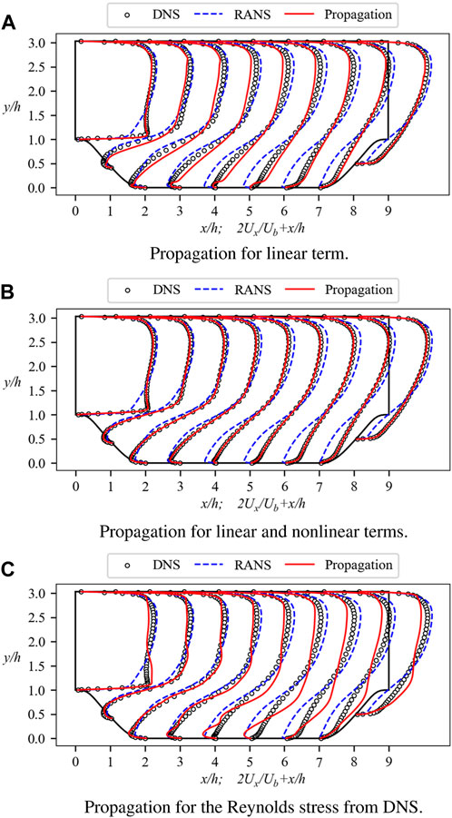
Figure 1. Mean streamwise velocity profiles for the propagation test at Re = 5600 and α = 1.0. The profiles are displayed at nine streamwise locations x/h = 0, 1, 2, …, 8. Baseline RANS simulations and DNS results are included for comparison. (A) Propagation for linear term. (B) Propagation for linear and nonlinear terms. (C) Propagation for the Reynolds stress from DNS.

However, the propagation test displays some improvements in velocity, notably high consistency with DNS on the windward side. Each profile indicates that the velocity propagated by the linear term maintains a similar trend to DNS. Despite these improvements, the velocity propagated solely from ${\nu }_t^{*}$ exhibits discrepancies, particularly near the lower wall. From x/h = 3 to x/h = 5, the velocities prematurely transition to positive values, as displayed on the velocity profile, showing a small bump towards the left. This underscore the limitations of relying solely on the linear term to accurately obtain Reynolds stresses, as velocities calculated using the linear term still exhibit significant errors. The relationship between Reynolds stress and strain rate tensor cannot be simply regarded as linear, highlighting the limitations of LEVMs.

Additionally, we plot the difference between the Reynolds stress anisotropy tensor a and the linear term in Figure 2. In the propagation test, the Reynolds stress is approximated by the linear term, i.e., $\mathit{a}=2{\nu }_t^{*}{\mathit{S}}^{\text{DNS}}$. As this work focuses on two-dimensional flow, the errors in a₁₁, a₁₂, and a₂₂ are presented here. Since a is the zero-trace tensor (i.e., a₁₁ + a₂₂ + a₃₃ = 0), Figure 2 also displays the non-zero a₃₃. The results indicate that the error in the flow separation zone is most pronounced. All four components featured in Figure 2 exhibit substantial errors near the lower wall, correlating with the anomalous velocity observed in Figure 1A. This implies that these errors significantly influence the velocity prediction.

Figure 2

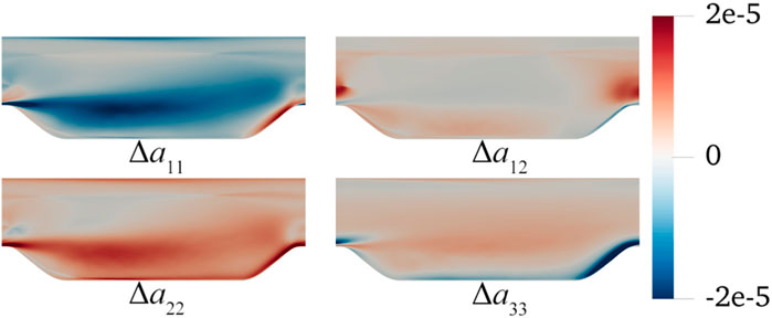
Figure 2. Errors in the Reynolds stress anisotropy tensor a approximated by optimal eddy viscosity for four components. The errors are calculated as $\mathrm{\Delta }\mathit{a}={\mathit{a}}^{\text{DNS}}-2{\nu }_t^{*}{\mathit{S}}^{\text{DNS}}$.

It has been established that a cannot be accurately reproduced solely through a linear relationship. To enhance the velocity prediction, the introduced nonlinear term, denoted as a^⊥ hereafter, is derived from the discernible correlation between Δa and velocity. Thus, the Reynolds stress anisotropy tensor, incorporating the linear term and nonlinear a^⊥, is expressed as:

$\mathit{a}=2{\nu }_t^{*}\mathit{S}+{\mathit{a}}^{\perp }.(10)$

By utilizing definition Eqs 2, 10 is reformulated as:

$\nabla \cdot \left(\mathit{U}\mathit{U}\right)-\nabla \cdot \left[\left(\nu +{\nu }_t^{*}\right)\left(\nabla \mathit{U}+{\left(\nabla \mathit{U}\right)}^{\text{T}}\right)\right]=-\nabla p^{\prime }+\gamma \nabla \cdot {\mathit{a}}^{\perp },(11)$

where γ is a scaling factor determined by minimizing the mean square error between propagation and DNS velocity, detailed in Section 3.5. Eq. 11 will be used in the second propagation test. Compared to Eq. 4, the only modification is the addition of a term on the right side of the equation. This term remains constant in the propagation test and serves as a corrective measure. The current Reynolds stress anisotropy tensor is divided into linear and nonlinear parts, both of which can be obtained directly from the high-fidelity data. Since we have already calculated the linear term using Eq. 9, the nonlinear term can be determined as ${\mathit{a}}^{\perp }=\mathit{a}-2{\nu }_t^{*}\mathit{S}$.

To assess the effectiveness of this approach, a new propagation test using Eq. 11 is conducted, as depicted in Figure 1B. It is clear that the propagated velocity has been greatly improved compared to Figure 1A. The previously observed underestimation of velocity near the upper wall has been addressed, and the flow separation region, which exhibited the most severe error in Figure 1A, also shows significant improvement in Figure 1B. The position of the separation bubble tends to align with DNS, and the small protrusion of velocity near the lower wall has disappeared. Based on these comparisons, it becomes evident that the inclusion of the nonlinear term is crucial for accurate velocity prediction.

We also explore the direct substitution of Reynolds stress. Although we have decomposed a into two terms, it raises the question: what would happen if we directly inserted the entire a from DNS into Eq. 2? By incorporating the complete a directly, the presence of ν_t would be eliminated, fundamentally altering the essence of the LEVM. Nevertheless, contemplating this possibility serves to highlight the advantages of Eq. 10. By replacing a^⊥ on the right side of Eq. 11 with a^DNS and removing ${\nu }_t^{*}$ on the left side, we can perform another propagation test. The resulting outcomes are depicted in Figure 1C. During this process, we encounter challenges in achieving convergence, with large fluctuations in velocity. Figure 1C displays the profiles at a certain time during the velocity fluctuations, which are even less effective than the baseline simulation. This reaffirms the effectiveness of the nonlinear term. This issue was also discussed by Thompson et al. [53], Wu et al. [45], who proposed that the explicit insertion of Reynolds stress can make the RANS equation ill-conditioned. In their work, Wu et al. [45] introduced a condition number, delving into the drawbacks of an explicit closure term, while affirming the efficacy of the implicit substitution method.

Up to this point, the corrected velocity has been obtained under ideal conditions, where the Reynolds stress used for calculations is directly derived from DNS. Alongside ${\nu }_t^{*}$ being identified as a learning target, several components of a^⊥ will also be treated as additional learning targets. These target quantities will be predicted using a specific machine learning algorithm, with the results presented in this section serving as the upper limit for the data-driven model.

2.4 Model framework

In summary, this study aims to enhance the prediction capability of the k-ω SST model. Through verification, the RANS closure term composed of linear and nonlinear terms can effectively reduce the prediction errors and closely reproduce the DNS velocity. The overall model framework will be elaborated in this section.

As illustrated in Figure 3. It consists of two distinct phases: the training and the prediction phase, which are independent of each other. In the training phase, we employ supervised learning, with ${\nu }_t^{*}$ and a^⊥ as labels, and the inputs are derived from the mean field obtained by the baseline simulation. The training process involves solving a regression problem, which concludes when the discrepancy between the predicted and target values reaches a specific threshold.

Figure 3

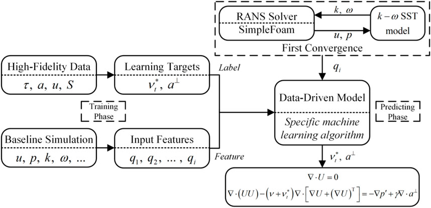
Figure 3. Framework of the current data-driven model.

During the prediction phase, the trained model is integrated into the CFD calculation. When the baseline simulation converges, the data-driven model makes predictions. A modified RANS solver calculates the features and passes them to the data-driven model. The predicted ${\nu }_t^{*}$ and a^⊥ are then utilized in solving the momentum equation. Propagation tests have demonstrated that several thousand time steps are required for the modified closure term to converge. Taking this into account, we adopt a “one-time correction” approach, as suggested by Ho and West [54]. This approach operates as an open-loop control, where the data-driven model is invoked only once at a chosen moment, and the predicted values are frozen and incorporated into the calculation until convergence is reached. Another iterative framework used by Liu et al. [35] involves repeated invocations of the model, using predicted values from each iteration in subsequent predictions. However, given the high number of iterations required in the propagation tests, small errors that might arise within iterative frameworks could be amplified. Hence, the current research adopts the open-loop control approach to mitigate the potential amplification of such errors, which is also influenced by the need for stability and certainty in the results produced by the model.

The propagation tests for the present study, as well as the baseline simulations, are conducted using the finite volume open-source CFD code, OpenFOAM. We utilize the simpleFoam solver, which is designed for steady incompressible Newtonian fluids. The modified simpleFoam solver incorporates Eq. 11 and is capable of computing features while invoking the data-driven model.

3 Machine learning algorithm

3.1 Neural networks

In the present work, neural networks are applied to predict the closure term. A neural network is a mathematical or computational model designed to replicate the structural and functional dynamics of biological neural networks, particularly the central nervous system of animals, such as the brain. These models are employed to approximate or estimate functions without the need for deriving explicit functional relationships. Neural networks can be perceived as a black boxes that establish a mapping relationship between specific features and labels.

A typical neural network comprises an input layer, an output layer, and several hidden layers. The input layer receives the specific features, and the network is updated by minimizing the difference between the output layer and the labels. Neurons are the fundamental components of a neural network, and each neuron receives n inputs from the previous layer, all of which are weighted. An activation function processes the sum of these inputs, combined with a bias term, to produce the neuron’s output. It can be mathematically represented as Eq. 12.

$z=h\left({\displaystyle \sum _{i=1}^n}{\omega }_i{x}_i+b\right),(12)$

where x denotes the inputs from the previous layer, h denotes the activation function, and ω and b represent the weight and bias, respectively.

In this study, two distinct neural networks, N1 and N2, are trained to predict the linear and nonlinear terms, respectively. N1 is utilized to predict the linear term ${\nu }_t^{*}$, while N2 is employed to predict the nonlinear term a^⊥. Despite using the same input features, N1 and N2 differ in their network structure and hyperparameters. The number of neurons in each layer is proportional to the number of input features, denoted as N_q. For N1, the network structure is N_q − 6N_q − 12N_q − 6N_q − 6N_q − 2N_q − N_q. Similarly, for N2, it is N_q − 6N_q − 12N_q − 6N_q − 2N_q − 3N_q. A more complex network structure has the potential to capture complex mapping relationships better; however, it also increases the risk of overfitting. To strike a balance, the current network design is chosen with appropriate complexity and minimized overfitting risk.

The choice of activation function is critical as it introduces nonlinearity between layers of neurons, enabling the learning of complex models, which is essential given the nonlinear nature of most real-world problems. For both N1 and N2, the Rectified Linear Unit (ReLU) function is selected as the activation function, defined as Eq. 13.

$f\left(x\right)=\max \left(0,x\right).(13)$

To optimize the neural networks, both N1 and N2 employ the Adam optimizer [55]. For N1, the learning rate is set to 5 × 10⁻⁵, and L2 regularization is applied with a regularization coefficient λ = 1 × 10⁻⁵. For N2, the learning rate is set to 1 × 10⁻⁴, with L1 regularization in use with a regularization coefficient λ = 1 × 10⁻⁵.

The implementation of N1 and N2 is carried out using the open-source neural network framework, PyTorch [56], owing to its outstanding flexibility and user-friendly interface. As training and prediction are separate processes, N1 and N2 are trained independently outside OpenFOAM. The trained neural networks are saved as TorchScript models, which provide an intermediary representation of the PyTorch model capable of execution in C++ code. By importing the TorchScript model into OpenFOAM, the trained neural networks can be invoked within the RANS solver. This separation of training and prediction significantly enhances work efficiency and facilitates the integration of the data-driven model into the computational framework.

3.2 Features for neural networks

Throughout the history of data-driven turbulence model development, the selection of input features has remained a pivotal concern during the model training phase. Input features are instrumental in recognizing and characterizing the flow field and its associated structures. Turbulence properties are highly complex, involving the interaction and evolution of multiple physical quantities. Therefore, for an accurate prediction of turbulent field behavior, the selection of input features must incorporate considerations of flow variables and their physical implications.

However, from a data perspective, acquiring and processing certain physical quantities can be expensive and computationally intensive. Hence, considerations of data availability and computational efficiency must guide the selection and extraction process of input features. Additionally, the concept of generalization performance is essential, as it ensures the model’s ability to generalize to unfamiliar data. It is crucial to establish a consistent form of input features that can be obtained across diverse datasets. While increasing the number of input features can enhance prediction performance, it may also lead to training complexities and excessive consumption of computational resources. Therefore, feature selection should strike a balance between physical relevance, data availability, interpretability, and computational efficiency.

In this study, two types of input features have been utilized. One type is derived from Ling et al. [57], where inputs with invariance are generated by constructing integrity bases. The other type is based on empirical knowledge and constructed from mean flow quantities. Inspired by Wu et al. [27], we adopt the minimal integrity basis for constructing the input features. To simplify the model and facilitate trailing, we choose to utilize only the strain rate tensor S and rotation rate tensor Ω to construct the minimal integrity basis, resulting in a reduced number of invariant bases (6 in total). The input features for N1 and N2 are delineated in Table 1.

Table 1

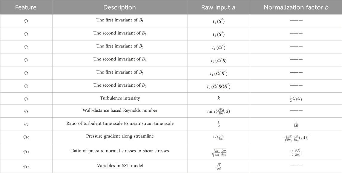
Table 1. Input features for neural networks.

The features q₁-q₆ listed in Table 1 satisfy Galilean invariance, where $\widehat{\mathit{S}}=\frac{1}{2}\frac{k}{ϵ}(\nabla \mathit{U}+{(\nabla \mathit{U})}^{\text{T}})$ and $\widehat{\mathbf{\Omega }}=\frac{1}{2}\frac{k}{ϵ}(\nabla \mathit{U}-{(\nabla \mathit{U})}^{\text{T}})$ represent the dimensionless strain rate tensor and rotation rate tensor, respectively. In the two-dimensional flow setting, the first invariants of tensor bases B₂, B₄ and B₆ are equal to zero, leading us to adopt the second invariants as the input features. The occurrence of both separation bubble and reverse flow can be attributable to the pressure gradient, which is incorporated into q₁₀ and q₁₁. Additionally, turbulence kinetic energy is a crucial parameter for describing turbulent properties. To enhance the precision of flow separation prediction, turbulence kinetic energy is included in q₇, q₈, and q₁₂. As we have observed in the previous discussions, the linear and nonlinear terms close to the lower wall significantly impact velocity prediction. Therefore, the inclusion of wall distance in q₈ is expected to play a significant role in near-wall prediction. Furthermore, considering that the “improvement” is targeted at the k-ω SST model, we introduce the specific dissipation rate ω into q₉ and q₁₂. Compared to the research conducted by Wu et al. [27], the minimal integrity basis no longer includes pressure gradient and turbulence kinetic energy, effectively reducing the total number of input features to 12, thereby simplifying the task for neural networks.

3.3 Normalization of input features

The input features outlined in Table 1 exhibit significant variations that span multiple orders of magnitude, potentially impeding the training process. This wide range of magnitudes among the features results in an unequal influence on prediction outcomes, causing the neural network to be more biased towards features with larger weights during training. Since neural networks rely on the gradient descent method for training, the presence of features with diverse magnitudes requires more iterations to update network parameters effectively. Moreover, the distribution of input features also impacts model performance, and data scaling can assist algorithms in discovering more effective patterns within the data while mitigating interference from anomalous values. Therefore, about the work completed by McConkey et al. [46], the features listed in Table 1 will undergo normalization.

The tensor bases of q₁-q₆ are normalized using the turbulent time scales k/ϵ, while no processing is necessary for q₈ and q₁₂. The remaining four features are normalized using $\widehat{a}=a/b$, where a is derived from the raw input and b is obtained from the normalization factor outlined in Table 1. It is important to note that these normalization factors are specific to local quantities obtained from grid points. To reduce sensitivity to magnitude differences in the data, the normalized features $\widehat{a}$ are compressed using $q^{*}=\log (|\widehat{a}|+1)$. Here, $\widehat{a}$ encompasses both the raw inputs q₁-q₆, q₈, q₁₂ and the normalized inputs. Subsequently, all features are transformed to a range of $\left[0,+\infty \right)$. The final step involves converting q* into the range $\left[\mathrm{0,1}\right]$ using the MinMaxScalar method. The actual input feature obtained through MinMaxScalar is given by Eq. 14.

$q_i=\frac{q_i^{*}-\min \left(q_i^{*}\right)}{\max \left(q_i^{*}\right)-\min \left(q_i^{*}\right)}.(14)$

3.4 Labels for neural networks

In the preceding discussions, it has been ascertained that the learning targets encompass both the linear and nonlinear components of the closure term. Network N1’s label is identified as ${\nu }_t^{*}$, while network N2’s label is identified as a^⊥. The nonlinear term comprises four non-zero components; however, due to the approximation $a_{11}^{\perp }+a_{22}^{\perp }+a_{33}^{\perp }\approx 0$, only three components need to be determined.

The term ${\nu }_t^{*}$ is computed using Eq. 9. Upon obtaining ${\nu }_t^{*}$, the term a^⊥ can be calculated through ${\mathit{a}}^{\perp }=\mathit{a}-2{\nu }_t^{*}\mathit{S}$. ${\nu }_t^{*}$ is normalized by the molecular kinematic viscosity ν from DNS. The maximum value of the normalized term ${\nu }_t^{*}/\nu$ remains on the order of several thousands, necessitating compression treatment with ${\nu }_t^{\mathit{label}}=\log ({\nu }_t^{*}/\nu +1)$. Subsequently, the term ${\nu }_t^{\mathit{label}}$ processed using the MinMaxScalar method is employed as the label for N1.

The normalization of a^⊥ differs slightly in that the compression treatment log (|x| + 1) is no longer required. This is because the nonlinear term signifies the discrepancy between the linear term and the Reynolds stress anisotropy tensor, requiring accurate quantification of both positive and negative values. a^⊥ is normalized by the bulk velocity U_b, which serves as an artificially assigned initial condition for driving periodic hills flows. The resulting normalized nonlinear term is expressed as ${\mathit{a}}^{\perp }/(\frac{1}{2}{\mathit{U}}_b{\mathit{U}}_b)$, subsequently serving as the label for N2 after undergoing the MinMaxScalar process. In practice, the three components of a^⊥ are treated separately, just like the process for ${\nu }_t^{*}$.

3.5 Dataset

The propagation tests and training of the neural network discussed above are conducted with the flow over 2D periodic hills. The computational domain and boundary conditions for this specific flow configuration are illustrated in Figure 4. Cyclic boundary conditions are applied to the inlet and outlet boundaries, and the flow is driven by a constant applied body force. The height of the periodic hills, denoted as h, is chosen as the characteristic length scale, and the Reynolds number is defined as Re = U_bh/ν, where U_b represents the bulk velocity attained through the controlling body force. The height of the computational domain is set to 3.06h. The length of the computational domain is determined by the scaling factor α, representing the steepness of the hills.

Figure 4

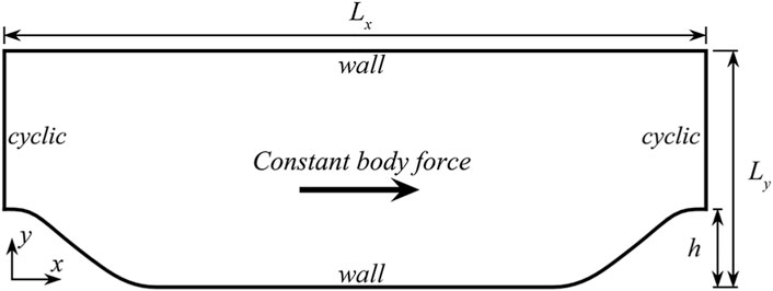
Figure 4. Computational domain for 2D periodic hill flows. The hill height is represented by h. The x and y coordinates correspond to the streamwise and wall-normal directions, respectively.

Figure 5 presents a range of geometries for the flow over periodic hills. The data corresponding to α = 1.5 and α = 1.0 are utilized for training the neural networks, while those associated with α = 1.2 and α = 0.8, 0.5 serve for interpolation and extrapolation tests, respectively. Baseline RANS simulations are conducted for each α to extract the 12 input features from the mean flow field. These baseline simulations employ the steady-state solver “simpleFoam” with the open-source platform OpenFOAM v2112.

Figure 5

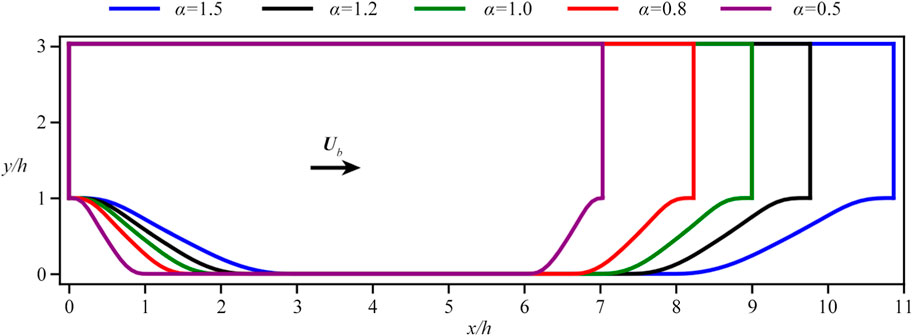
Figure 5. The profiles for different periodic hills considered in the current study, with their scaling factors α = 0.5, 0.8, 1.0, 1.2, 1.5 (from left to right).

The high-fidelity data with varying α are provided by Xiao et al. [58]. Both RANS and DNS simulations are performed at a fixed Reynolds number of Re = 5600. In the dataset by Xiao et al. [58], DNS simulations are carried out on a more refined grid, and the obtained results are subsequently mapped onto a coarser RANS grid with an identical geometry. Throughout the simulation of these four distinct geometries, an equal number of grid cells is employed, with each grid containing 14,751 cells $\left(99\times 149\right)$, which have been validated by Xiao et al. [58]. During the training phase, the labels are calculated using the velocity and Reynolds stress fields extracted from the DNS dataset.

In the derivation of Eq. 11 in Section 2.3, we introduce a scaling factor γ as a modulation parameter. As discussed above, the inclusion of the nonlinear term serves the crucial role of modulating the discrepancies introduced by the linear term. It is observed that the modulation effect can be controlled through the manipulation of the scaling factor γ, leading to better predictions. The determination of an appropriate range for γ involves comprehensive assessments on flow characteristics over varying geometries of periodic hills. A comprehensive suite of 55 simulations is conducted, encompassing a spectrum of γ values spanning from 1 to 2. These simulations are performed across diverse flow scenarios over periodic hills characterized by different α values. The efficacy of the approach is evaluated using the momentum Eq. 11, and the Mean Squared Error (MSE) of the velocity field serves as the primary criterion for evaluation, defined as

$U_{\text{MSE}}=\frac{1}{n}{\displaystyle \sum _{i=1}^n}{\left(\mathit{U}-{\mathit{U}}_{\text{DNS}}\right)}^2,(15)$

where, n represents the number of grid points.

The results of the tests are presented in Figure 6. Across the five distinct test sets, a consistent trend is evident—initial reduction followed by subsequent elevation of MSE with increasing γ. The extent of MSE variation is more pronounced for higher α values. As an illustrative example, for α = 0.5, MSE varies within the confined range of 0.5 × 10⁻⁶ to 0.8 × 10⁻⁶. Notably, within the γ interval of 1.0–1.4, a marginal yet consistent decrement in MSE is observed, though with relatively modest magnitudes. In contrast, for α = 1.5, the MSE spans a broader spectrum of 0.1 × 10⁻⁶ to 1.7 × 10⁻⁶. This divergence underscores the heightened sensitivity of calculations to γ when the hill slope diminishes. Drawing from the comprehensive analysis of the 55 cases, an optimal γ range is determined to be $\left[1.4,1.6\right]$. Within this interval, the velocity computed through Eq. 11 exhibits the least deviation in comparison to DNS. Deliberating upon both training and testing scenarios, we opt for a value of γ = 1.5 in the present study.

Figure 6

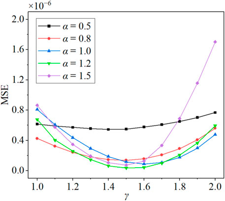
Figure 6. The trend of the mean square error of velocity with the scaling factor γ. The curves represent the variations under five different geometric structures.

4 Numerical results

4.1 Training of neural networks

The two neural networks, N1 and N2, are trained using a dataset that encompasses both the baseline RANS data and the high-fidelity DNS data. During the training process, optimization algorithms are employed to adjust the weights and biases in the neural network with a batch size of 1,024. The Adam optimizer, based on the gradient descent method, is utilized. Its primary concept is to employ the mean and squared mean of the gradient to estimate an adaptive learning rate. Before training, the data associated with α = 1.0 and 1.5, designated for training, are randomly shuffled. Subsequently, approximately 90% the shuffled data is allocated to the training set, while the remaining 10% forms the validation set. In addition, the data associated with α = 0.5, 0.8, 1.2 are used for testing.

A regularization strategy is employed during training to mitigate multicollinearity. The L2 regularization strategy is applied to N1 during training, which entails a loss function defined as Eq. 16.

$Loss=\frac{1}{n}{\displaystyle \sum _{i=1}^n}{\left({\widehat{y}}_i-y_i\right)}^2+\frac{\lambda }{2n}{\displaystyle \sum _{i=1}^n}{\left|{\omega }_i\right|}^2,(16)$

where n is the total number of neurons, ${\widehat{y}}_i$ denotes the predicted value, and y_i represents the label. ω corresponds to the weight of each neuron, and λ represents the regularization coefficient. Initial values of neural network weights and biases are assigned randomly, which satisfy the normal distribution with the expected value of zero. Both N1 and N2 undergo multiple training cycles using the aforementioned method, with the best-performing model being selected. The losses of N1 and N2 during the training process are illustrated in Figure 7.

Figure 7

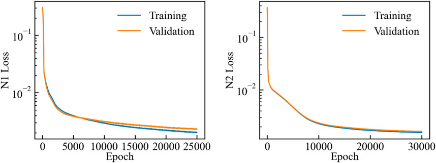
Figure 7. The progression of losses during the training process for N1 and N2.

The trend in Figure 7 confirms that the training of N1 has successfully converged. Notably, the decline in loss is synchronized between the training and the validation sets, a phenomenon that persists even beyond 25,000 epochs. However, it is crucial to recognize that pursuing further epochs could introduce the risk of overfitting. Consequently, a judicious decision is made to conclude the training process at the 25000th epoch. Similarly, we note that N2 reaches convergence around the 30000th epoch, beyond which the loss on the validation set stabilize, indicating a prudent halting point for training. While the loss curve for the validation set frequently dips below that of the training set during the training process, further evaluations reveal that stopping training around the 25000th epoch yields superior predictive and generalization capabilities.

4.2 Predictive performance of neural networks

4.2.1 Predictive performance of closure term

A critical metric for assessing the performance of machine learning models is their generalization capability. While achieving accurate predictions on the training set is imperative, the true value of these models lies in their ability to perform effectively on previously unseen data. We have utilized cases with α = 1.0, 1.5 for training. In this section, we will proceed to evaluate the model’s performance when applied to the case with α = 1.2.

The statistical assessment of the testing case with α = 1.2 is depicted in Figure 8. The resemblance in distribution trends between the predicted and true values is evident, and the symmetry of the error distribution underscores the absence of indications pointing towards overfitting within the two models. Notably, $a_{12}^{\perp }$ displays a distribution with a heightened concentration and a reduced prediction error, relative to the other two components. This observation indicates N2’s enhanced capacity for reliable shear stress predictions, with the 12 chosen input features evidently demonstrating a more robust correlation with shear stress.

Figure 8

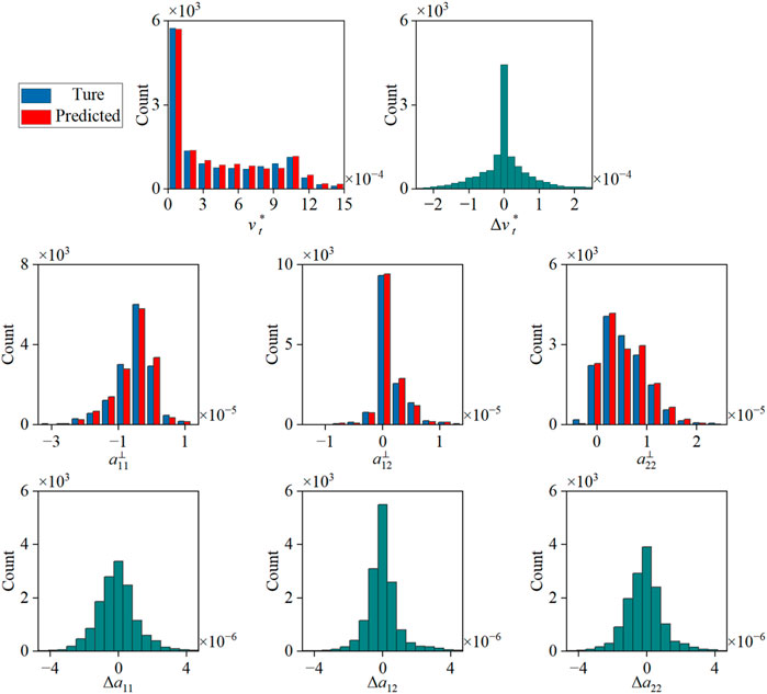
Figure 8. Statistical evaluations of N1 and N2 predictions for the α = 1.2 testing case.

As the ML is used to predict linear and nonlinear terms of the Reynolds stress anisotropy tensor, the sum of both must match to a certain extent. To facilitate a more intuitive comprehension of the closure term, we combine the linear and nonlinear terms to constitute the Reynolds stress anisotropy tensor, as presented in Figure 9. This visual representation elucidates that the performance of the k-ω SST model in approximating the closure term is dissatisfactory. Among the three components depicted, the k-ω SST model manifests trend-consistent outcomes with the DNS data solely in the context of a₁₂. Regarding a₁₁ and a₂₂, the k-ω SST model computes extreme values that are antithetical to those observed within the DNS data. In contrast, our ML model delivers accurate predictions, notably in the middle region of the computational domain. Within the vicinity of flow separation, the ML model demonstrates a heightened accuracy in predicting the Reynolds stress anisotropy tensor. While specific areas within the predictions might experience overestimation, they persist within an acceptable range. However, we note that predictions of network are grid-specific, and when considering the entirety of the flow domain, certain instances of discontinuity may arise. This phenomenon is a prevalent challenge in the application of machine learning to physical modeling. Thankfully, when we propagate the Reynolds stresses to the mean velocity field, this discontinuity does not exert a significant impact on the velocity predictions, just as shown in Section 4.2.2.

Figure 9

Figure 9. Comparison of the Reynolds stress anisotropy tensor a for the α = 1.2 testing case among DNS, ML, and RANS data. The predicted value is a combination of linear and nonlinear terms predicted by models N1 and N2. RANS data is extracted from the baseline simulation using the k-ω SST model.

4.2.2 Predictive performance of mean field

It remains to be tested whether the Reynolds stress predicted by the neural networks is effective when integrated to predict the mean field.

Figure 10 presents the computed mean velocity field, Utilizing Eq. 11. Figure 10A specifically illustrates the substantial enhancement in the streamwise velocity component. As previously mentioned, the outcomes featured in Figure 1A can be regarded as an upper-bound prediction limit. The current velocity profiles eloquently illustrate the proximity of the generalization test outcomes to this upper limit. Noteworthy differences emerge in the upper region of the computational domain, wherein the k-ω SST model generates overestimated velocity predictions, subsequently rectified by the ML model’s corrections. In the flow separation region, the k-ω SST model yields underestimated velocity predictions, whereas the ML model’s predictions more aptly align with the DNS data. Near the lower wall, the k-ω SST model predicts an elongated reverse flow in the streamwise direction, a shortcoming not evident in the ML model’s predictions. Along the right slope, characterized by a narrowing channel width, the ML model exhibits a commendable prediction performance. Particularly noteworthy is its capacity to accurately predict the rapid velocity escalation near the apex (x/h = 0), wherein the ML model distinctly surpasses the predictive performance of the k-ω SST model.

Figure 10

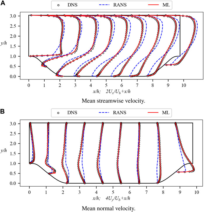
Figure 10. Mean velocity profiles for the α = 1.2 testing case. The profiles are shown at nine streamwise locations x/h = 0, 1, 2, …, 8. Baseline RANS simulations and DNS results are also included for comparison. (A) Mean streamwise velocity. (B) Mean normal velocity.

The ML model also performs well for the normal velocity, as depicted in Figure 10B. The k-ω SST model exhibits under-prediction across the entirety of the computational domain. Although the k-ω SST model correctly captures the direction of the normal velocity, discernible disparities arise in terms of magnitude. This discrepancy is effectively rectified by the ML model, which mitigates the error and enhances the overall conformity to the reference data. For a quantitative assessment, we have conducted MSE computations of velocity for both models, as outlined in Eq. 15. The ensuing results unveil an error magnitude of 3.98 × 10⁻⁷ for the ML model and 1.14 × 10⁻⁵ for the k-ω SST model.

In addition to velocity, we also examine derived quantities, such as the wall shear stress, an entity tightly correlated with flow separation. The computation of wall shear stress derives from the velocity gradient of the first layer grid near the wall. Figure 11 displays the skin friction coefficient along the lower wall, characterized as the ratio of the wall shear stress to the dynamic pressure of the free flow. As observed in this figure, the ML model provides predictions closely aligned to the DNS data, thereby offering additional affirmation for its adeptness in predicting separation bubbles. Another derived quantity of the mean velocity gradient, y⁺, is also calculated. The mean y⁺ corresponding to DNS, ML and k-ω SST model are 0.370, 0.362, and 0.353 respectively. Clearly, in contrast to the k-ω SST model, the ML model consistently delivers precise prognoses for flow separation and reattachment points.

Figure 11

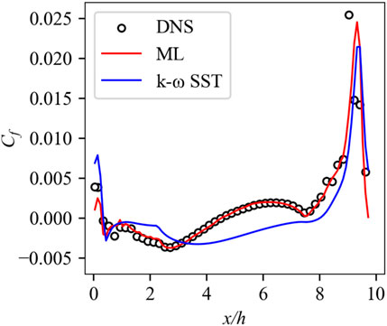
Figure 11. Skin friction coefficient along the bottom wall for the α = 1.2 testing case.

4.3 Extrapolation test

The ML model has exhibited favorable performance in the testing case with α = 1.2, wherein the geometry can be regarded as an interpolation within the training set. However, a critical aspect is to evaluate the ML model’s performance when applied to cases that deviate from the training set. The examination in this section involves the extrapolation tests performed on the α = 0.8, 0.5 cases.

As depicted in Figure 5, the α = 0.8 case presents shorter computational domain lengths and steeper hills. By integrating the closure terms predicted by N1 and N2 into the velocity field, the resultant streamwise velocity profiles are depicted in Figure 12A. The ML model displays superior predictive capabilities compared to the k-ω SST model. Specifically, along the windward side of the right hill, the ML model provides accurate predictions as expected. This includes the hill crest at x/h = 0, where the ML model remarkably predicts the rapid growth rate. Furthermore, in the upper part of the computational domain, the ML model demonstrates enhanced accuracy, consistent with earlier observation. The MSE values of velocity have been computed for both models using Eq. 15, resulting in 9.34 × 10⁻⁷ for the ML model and 4.79 × 10⁻⁶ for the k-ω SST model. Overall, in the unfamiliar case, the ML model delivers satisfactory predictions, indicating that N1 and N2 can adeptly assimilate limited data and generate reasonable inferences.

Figure 12

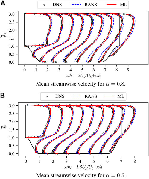
Figure 12. Mean streamwise velocity profiles for the α = 0.8, 0.5 testing case. The profiles are shown at nine streamwise locations x/h = 0, 1, 2, …, 8. Baseline RANS simulations and DNS results are also included for comparison. (A) Mean streamwise velocity for α = 0.8. (B) Mean streamwise velocity for α = 0.5.

Figure 13 provides insight into the error distribution of the ML model and the k-ω SST model, wherein the error is defined as $U_x^{\mathit{DNS}}-U_x$. Evidently, the k-ω SST model tends to over-predict, resulting in errors primarily concentrated on both sides away from 0. In contrast, the ML model exhibits a more symmetric distribution around 0, signifying that the machine learning errors exhibit randomness. This suggests that by increasing the amount of training data, these errors can be further minimized.

Figure 13

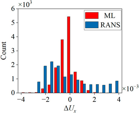
Figure 13. Prediction error $\mathrm{\Delta }{U}_x=U_x^{\mathit{DNS}}-U_x$ of the ML and the RANS models for the α = 0.8 testing case.

Furthermore, the α = 0.5 case represents a more challenging scenario, with the resultant prediction illustrated in Figure 12B. Notably, the distinctions among the three curves presented in this figure are mitigated in comparison to the preceding cases. Directing our attention solely to the predictions of the ML model, it demonstrates a favorable concordance with the DNS data. Within this geometric configuration, the k-ω SST model also exhibits proximity to the DNS data, although this proximity should not be misconstrued as a precise prediction of flow separation. Extensive calculations have unveiled the inadequacies of the k-ω SST model in the context of complex flows, despite its capacity to yield approximate outcomes under specific circumstances.

Figure 14 presents the streamwise velocity contours of the entire flow field for three testing cases, accompanied by streamlines that offer visual comparison of flow characteristics. The k-ω SST model engenders an excessively expanded separation bubble, with its center located further downstream. In contrast, the ML model accurately captures the dimensions of the separation bubble, closely aligning with the DNS data, and positions its center closer to the slope. However, as observed in this figure, the k-ω SST model tends to overestimate the extent of separation bubbles when the dimensions of these bubbles are smaller than the intervals between the periodic hills. As the α decreases, thereby steepening the slope, the separation bubbles exhibited by the DNS data show a tendency for grow. Coinciding with the diminishment of the channel length, the disparity between the DNS and k-ω SST models decreases with the decrease in α. Consequently, in this particular instance, the disparities between the k-ω SST model and DNS are relatively modest.

Figure 14

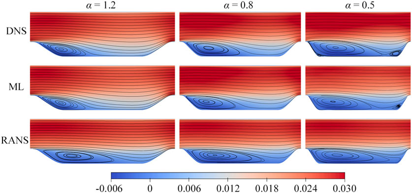
Figure 14. Contours of mean streamwise velocity for the α = 1.2, 0.8, 0.5 testing case. The distinct separate bubbles from DNS, ML model, and RANS simulations are represented by streamlines.

We designate the situation where α = 0.5 as “challenging,” given its manifestation of attributes that extend beyond the scope of the training cases. As depicted in Figure 14, the separation bubble in this instance connects two hills, a phenomenon not previously encountered in the training cases. A diminutive reverse vortex structure becomes discernible between the separation bubble and the left slope, presenting a hurdle for the accurate prediction of the near-wall region. Regrettably, the ML model’s prediction in Figure 12B fares poorly at this location. Nevertheless, remarkably, the ML model’s prediction extends beyond the confines of the training set to a certain degree. Noteworthy is the presence of a smaller separation bubble in the DNS data of Figure 14, shed off from the tail of the larger bubble, a feature absent from the training set. However, the ML model captures a similar configuration, thereby substantiating its capacity for extrapolation. In summation, the predictive efficacy of the ML model can be deemed satisfactory.

The extrapolation test undertaken in this section demonstrates the potential of the current ML model, which delivers accurate predictions even for challenging cases. While residual errors persist, it is posited that expanding the training dataset and incorporating a wider spectrum of geometric structures during the training phase will lead to further attenuation of these errors to a negligible level.

5 Conclusion

In this work, machine learning is employed to enhance turbulence modeling, aiming to refine the prediction capabilities of the RANS model while maintaining its computational efficiency. The widely adopted k-ω SST model serves as the foundational framework, and a data-driven approach is introduced to reconstruct the closure term. This reconstruction is achieved through neural network algorithms, leveraging high-fidelity data. The closure term is decomposed into linear and nonlinear components. The optimal eddy viscosity, denoted as ${\nu }_t^{*}$, is derived by minimizing the difference between the Reynolds stress anisotropy tensor a and the linear term, based on the Boussinesq assumption. The disparity between the linear term and a, designated as a^⊥, as a nonlinear correction, is incorporated into the momentum equation through an appropriate scaling factor. The determination of the appropriate scaling factor hinges on 55 simulation sets. Notably, propagation tests confirm the efficacy of the reconstructed closure term in enhancing the prediction of mean velocity.

We identify 12 key features from the minimal integrity basis and mean flow. These features facilitate the prediction of labels ${\nu }_t^{*}$ and a^⊥. Input features and labels are normalized to train the neural networks N1 and N2, which are designed to predict the linear and nonlinear terms, respectively. Data from periodic hills flows with different α values, signifying hill steepness, are employed. For training purposes, approximately 90% of the data with α = 1.0 and α = 1.5 are utilized, revering the remaining 10% for validation. The model’s generalization capability is gauged through interpolation tests employing the data with α = 1.2, and extrapolation tests utilizing the data with α = 0.8 and α = 0.5.

The ML model demonstrates notable precision in the α = 1.2 testing case. N1 and N2 exhibit satisfactory performance without showing a significant overfitting trend. The reconstructed closure term, a synthesis of the linear and nonlinear components, achieves augmented congruence with high-fidelity data in contrast to the k-ω SST model. By propagating this improved closure term to the mean field, the predictions correct the over-prediction anomalies associated with the k-ω SST model, thereby effectively containing the velocity error to an approximate margin of 1%. In the domain of flow separation, the ML model predicts a separation bubble that closely aligns with the high-fidelity data, whereas the k-ω SST model tends to exhibit an overestimation of its dimensions. Moreover, the ML model furnishes more precise prognostications of the flow reattachment point and showcases improved conformity with the lower wall skin friction coefficient.

The ML model consistently exhibits promising performance in extrapolation tests. In the case of α = 0.8, the ML model’s prediction aligns with DNS data, effectively rectifying the tendency of the k-ω SST model to overestimate. Similarly, in the more challenging α = 0.5 scenario, the ML model provides adept extrapolations. Although slight disparities between the k-ω SST model and DNS arise due to coincidence, the ML model adeptly anticipates the emergence of minor bubbles detaching from the primary separation bubble—a phenomenon not foreseen by the k-ω SST model.

The results presented herein underscore the efficacy of the current data-driven turbulence model, offering a refined closure term. This enhancement translates into improved predictions of velocity and its derived parameters, a critical aspect in engineering applications. This study extends the achievements of Wu et al. [27], wherein the PIML method demonstrated commendable predictive outcomes, accounting for intricate physical considerations. Here, we attain comparable achievements through a more concise neural network architecture, yielding superior velocity predictions within specific regions during both interpolation and extrapolation tests. In the future, the model’s accuracy and generalization potential can be further elevated through the augmentation of training data and expansion of the spectrum of flow geometries encompassed within the training regimen.

Data availability statement

The original contributions presented in the study are included in the article/Supplementary Material, further inquiries can be directed to the corresponding author.

Author contributions

ZC: Methodology, Formal Analysis, Writing–original draft. JD: Funding acquisition, Conceptualization, Writing–review and editing.

Funding

The author(s) declare financial support was received for the research, authorship, and/or publication of this article. This research has been supported by the National Natural Science Foundation of China (Grants Nos 92252102 and 92152109).

Conflict of interest

The authors declare that the research was conducted in the absence of any commercial or financial relationships that could be construed as a potential conflict of interest.

Publisher’s note

All claims expressed in this article are solely those of the authors and do not necessarily represent those of their affiliated organizations, or those of the publisher, the editors and the reviewers. Any product that may be evaluated in this article, or claim that may be made by its manufacturer, is not guaranteed or endorsed by the publisher.

References

1. Alfonsi G. Reynolds-averaged Navier–Stokes equations for turbulence modeling. Appl Mech Rev (2009) 62. doi:10.1115/1.3124648

CrossRef Full Text | Google Scholar

2. Durbin PA. Some recent developments in turbulence closure modeling. Annu Rev Fluid Mech (2018) 50:77–103. doi:10.1146/annurev-fluid-122316-045020

CrossRef Full Text | Google Scholar

3. Speziale CG. Analytical methods for the development of Reynolds-stress closures in turbulence. Annu Rev Fluid Mech (1991) 23:107–57. doi:10.1146/annurev.fl.23.010191.000543

CrossRef Full Text | Google Scholar

4. Shur ML, Strelets MK, Travin AK, Spalart PR. Turbulence modeling in rotating and curved channels: assessing the Spalart-Shur correction. AIAA J (2000) 38:784–92. doi:10.2514/2.1058

CrossRef Full Text | Google Scholar

5. Argyropoulos CD, Markatos N. Recent advances on the numerical modelling of turbulent flows. Appl Math Model (2015) 39:693–732. doi:10.1016/j.apm.2014.07.001

CrossRef Full Text | Google Scholar

6. Mishra AA, Duraisamy K, Iaccarino G. Estimating uncertainty in homogeneous turbulence evolution due to coarse-graining. Phys Fluids (2019) 31:025106. doi:10.1063/1.5080460

CrossRef Full Text | Google Scholar

7. Mishra AA, Girimaji S. Linear analysis of non-local physics in homogeneous turbulent flows. Phys Fluids (2019) 31:035102. doi:10.1063/1.5085239

CrossRef Full Text | Google Scholar

8. Eisfeld B. The importance of turbulent equilibrium for Reynolds stress modeling. Phys Fluids (2022) 34:025123. doi:10.1063/5.0081157

CrossRef Full Text | Google Scholar

9. Duraisamy K, Iaccarino G, Xiao H. Turbulence modeling in the age of data. Annu Rev Fluid Mech (2019) 51:357–77. doi:10.1146/annurev-fluid-010518-040547

CrossRef Full Text | Google Scholar

10. Brunton SL, Noack BR, Koumoutsakos P. Machine learning for fluid mechanics. Annu Rev Fluid Mech (2020) 52:477–508. doi:10.1146/annurev-fluid-010719060214

CrossRef Full Text | Google Scholar

11. Xiao H, Cinnella P. Quantification of model uncertainty in RANS simulations: a review. Prog Aerosp Sci (2019) 108:1–31. doi:10.1016/j.paerosci.2018.10.001

CrossRef Full Text | Google Scholar

12. Panda JP, Warrior H. Data-driven prediction of complex flow field over an axisymmetric body of revolution using machine learning. J Offshore Mech Arct Eng (2022) 144:060903. doi:10.1115/1.4055280

CrossRef Full Text | Google Scholar

13. Panda JP, Warrior HV. Evaluation of machine learning algorithms for predictive Reynolds stress transport modeling. Acta Mech Sin (2022) 38:321544. doi:10.1007/s10409-022-09001-w

CrossRef Full Text | Google Scholar

14. Zhu L, Zhang W, Kou J, Liu Y. Machine learning methods for turbulence modeling in subsonic flows around airfoils. Phys Fluids (2019) 31:015105. doi:10.1063/1.5061693

CrossRef Full Text | Google Scholar

15. Liu Y, Cao W, Zhang W, Xia Z. Analysis on numerical stability and convergence of Reynolds-averaged Navier–Stokes simulations from the perspective of coupling modes. Phys Fluids (2022) 34:015120. doi:10.1063/5.0076273

CrossRef Full Text | Google Scholar

16. Maulik R, Sharma H, Patel S, Lusch B, Jennings E. A turbulent eddy-viscosity surrogate modeling framework for Reynolds-averaged Navier-Stokes simulations. Comput Fluids (2021) 227:104777. doi:10.1016/j.compfluid.2020.104777

CrossRef Full Text | Google Scholar

17. Singh AP, Medida S, Duraisamy K. Machine-learning-augmented predictive modeling of turbulent separated flows over airfoils. AIAA J (2017) 55:2215–27. doi:10.2514/1.J055595

CrossRef Full Text | Google Scholar

18. Pochampalli R, Oezkaya E, Zhou BY, Suarez Martinez G, Gauger NR. Machine learning enhancement of Spalart-Allmaras turbulence model using convolutional neural network. AIAA Scitech (2021) 1017. doi:10.2514/6.2021-1017

CrossRef Full Text | Google Scholar

19. Wang Z, Zhang W. A unified method of data assimilation and turbulence modeling for separated flows at high Reynolds numbers. Phys Fluids (2023) 35:025124. doi:10.1063/5.0136420

CrossRef Full Text | Google Scholar

20. Jäckel F. A closed-form correction for the Spalart–Allmaras turbulence model for separated flows. AIAA J (2023) 61:2319–30. doi:10.2514/1.J061649

CrossRef Full Text | Google Scholar

21. Ling J, Templeton J. Evaluation of machine learning algorithms for prediction of regions of high Reynolds-averaged Navier-Stokes uncertainty. Phys Fluids (2015) 27:085103. doi:10.1063/1.4927765

CrossRef Full Text | Google Scholar

22. Ling J, Ruiz A, Lacaze G, Oefelein J. Uncertainty analysis and data-driven model advances for a jet-in-crossflow. J Turbomach (2017) 139:021008. doi:10.1115/1.4034556

CrossRef Full Text | Google Scholar

23. Ling J, Kurzawski A, Templeton J. Reynolds-averaged turbulence modelling using deep neural networks with embedded invariance. J Fluid Mech (2016) 807:155–66. doi:10.1017/jfm.2016.615

CrossRef Full Text | Google Scholar

24. Song X, Zhang Z, Wang Y, Ye S, Huang C. Reconstruction of RANS model and cross-validation of flow field based on tensor basis neural network. In: Fluids Engineering Division Summer Meeting; July, 2019; San Francisco, California, USA (2019).

CrossRef Full Text | Google Scholar

25. Parashar N, Srinivasan B, Sinha SS. Modeling the pressure-hessian tensor using deep neural networks. Phys Rev Fluids (2020) 5:114604. doi:10.1103/PhysRevFluids.5.114604

CrossRef Full Text | Google Scholar

26. Wang JX, Wu JL, Xiao H. Physics-informed machine learning approach for reconstructing Reynolds stress modeling discrepancies based on DNS data. Phys Rev Fluids (2017) 2:034603. doi:10.1103/PhysRevFluids.2.034603

CrossRef Full Text | Google Scholar

27. Wu JL, Xiao H, Paterson E. Physics-informed machine learning approach for augmenting turbulence models: a comprehensive framework. Phys Rev Fluids (2018) 3:074602. doi:10.1103/PhysRevFluids.3.074602

CrossRef Full Text | Google Scholar

28. Chang CW, Fang J, Dinh NT. Reynolds-averaged turbulence modeling using deep learning with local flow features: an empirical approach. Nucl Sci Eng (2020) 194:650–64. doi:10.1080/00295639.2020.1712928

CrossRef Full Text | Google Scholar

29. Xu R, Zhou XH, Han J, Dwight RP, Xiao H. A PDE-free, neural network-based eddy viscosity model coupled with RANS equations. Int J Heat Fluid Flow (2022) 98:109051. doi:10.1016/j.ijheatfluidflow.2022.109051

CrossRef Full Text | Google Scholar

30. Heyse JF, Mishra AA, Iaccarino G. Estimating RANS model uncertainty using machine learning. J Glob Power Propuls Soc (2021) 2021:1–14. doi:10.33737/jgpps/134643

CrossRef Full Text | Google Scholar

31. Zhang S, Li H, You R, Kong T, Tao Z. A construction and training data correction method for deep learning turbulence model of Reynolds-averaged Navier–Stokes equations. AIP Adv (2022) 12:065002. doi:10.1063/5.0084999

CrossRef Full Text | Google Scholar

32. Brenner O, Piroozmand P, Jenny P. Efficient assimilation of sparse data into RANS-based turbulent flow simulations using a discrete adjoint method. J Comput Phys (2022) 471:111667. doi:10.1016/j.jcp.2022.111667

CrossRef Full Text | Google Scholar

33. Tang H, Wang Y, Wang T, Tian L. Discovering explicit Reynolds-averaged turbulence closures for turbulent separated flows through deep learning-based symbolic regression with non-linear corrections. Phys Fluids (2023) 35. doi:10.1063/5.0135638

CrossRef Full Text | Google Scholar

34. Sanhueza RD, Smit SH, Peeters JW, Pecnik R. Machine learning for RANS turbulence modeling of variable property flows. Comput Fluids (2023) 255:105835. doi:10.1016/j.compfluid.2023.105835

CrossRef Full Text | Google Scholar

35. Liu W, Fang J, Rolfo S, Moulinec C, Emerson DR. An iterative machine-learning framework for RANS turbulence modeling. Int J Heat Fluid Flow (2021) 90:108822. doi:10.1016/j.ijheatfluidflow.2021.108822

CrossRef Full Text | Google Scholar

36. Liu W, Fang J, Rolfo S, Moulinec C, Emerson DR. On the improvement of the extrapolation capability of an iterative machine-learning based RANS framework. Comput Fluids (2023) 256:105864. doi:10.1016/j.compfluid.2023.105864

CrossRef Full Text | Google Scholar

37. Kaandorp ML, Dwight RP. Data-driven modelling of the Reynolds stress tensor using random forests with invariance. Comput Fluids (2020) 202:104497. doi:10.1016/j.compfluid.2020.104497

CrossRef Full Text | Google Scholar

38. Wu L, Cui B, Xiao Z. Two-equation turbulent viscosity model for simulation of transitional flows: an efficient artificial neural network strategy. Phys Fluids (2022) 34:105112. doi:10.1063/5.0104243

CrossRef Full Text | Google Scholar

39. Zhao Y, Akolekar HD, Weatheritt J, Michelassi V, Sandberg RD. RANS turbulence model development using CFD-driven machine learning. J Comput Phys (2020) 411:109413. doi:10.1016/j.jcp.2020.109413

CrossRef Full Text | Google Scholar

40. Frey Marioni Y, de Toledo Ortiz EA, Cassinelli A, Montomoli F, Adami P, Vazquez R. A machine learning approach to improve turbulence modelling from DNS data using neural networks. Int J Turbomach Propuls Power (2021) 6:17. doi:10.3390/ijtpp6020017

CrossRef Full Text | Google Scholar

41. Schmelzer M, Dwight RP, Cinnella P. Discovery of algebraic Reynolds stress models using sparse symbolic regression. Flow Turbul Combust (2020) 104:579–603. doi:10.1007/s10494-019-00089-x

CrossRef Full Text | Google Scholar

42. Huijing JP, Dwight RP, Schmelzer M. Data-driven RANS closures for three-dimensional flows around bluff bodies. Comput Fluids (2021) 225:104997. doi:10.1016/j.compfluid.2021.104997

CrossRef Full Text | Google Scholar

43. Zhang Y, Dwight RP, Schmelzer M, Gómez JF, Han Z, Hickel S. Customized data-driven RANS closures for bi-fidelity LES–RANS optimization. J Comput Phys (2021) 432:110153. doi:10.1016/j.jcp.2021.110153

CrossRef Full Text | Google Scholar

44. Cherroud S, Merle X, Cinnella P, Gloerfelt X. Sparse Bayesian learning of Explicit Algebraic Reynolds Stress models for turbulent separated flows. Int J Heat Fluid Flow (2022) 98:109047. doi:10.1016/j.ijheatfluidflow.2022.109047

CrossRef Full Text | Google Scholar

45. Wu J, Xiao H, Sun R, Wang Q. Reynolds-averaged Navier–Stokes equations with explicit data-driven Reynolds stress closure can be ill-conditioned. J Fluid Mech (2019) 869:553–86. doi:10.1017/jfm.2019.205

CrossRef Full Text | Google Scholar

46. McConkey R, Yee E, Lien FS. Deep structured neural networks for turbulence closure modeling. Phys Fluids (2022) 34:035110. doi:10.1063/5.0083074

CrossRef Full Text | Google Scholar

47. Guo X, Xia Z, Chen S. Computing mean fields with known Reynolds stresses at steady state. Theor Appl Mech Lett (2021) 11:100244. doi:10.1016/j.taml.2021.100244

CrossRef Full Text | Google Scholar

48. Guo X, Xia Z, Chen S. Practical framework for data-driven RANS modeling with data augmentation. Acta Mech Sin (2021) 37:1748–56. doi:10.1007/s10409-021-01147-2

CrossRef Full Text | Google Scholar

49. Volpiani PS, Meyer M, Franceschini L, Dandois J, Renac F, Martin E, et al. Machine learning-augmented turbulence modeling for RANS simulations of massively separated flows. Phys Rev Fluids (2021) 6:064607. doi:10.1103/PhysRevFluids.6.064607

CrossRef Full Text | Google Scholar

50. Berrone S, Oberto D. An invariances-preserving vector basis neural network for the closure of Reynolds-averaged Navier–Stokes equations by the divergence of the Reynolds stress tensor. Phys Fluids (2022) 34:095136. doi:10.1063/5.0104605

CrossRef Full Text | Google Scholar

51. Menter FR. Two-equation eddy-viscosity turbulence models for engineering applications. AIAA J (1994) 32:1598–605. doi:10.2514/3.12149

CrossRef Full Text | Google Scholar

52. Pasinato HD, Krumrick EA. Errors characterization of a RANS simulation. J Verif Valid Uncertain Quantif (2021) 6:021001. doi:10.1115/1.4050074

CrossRef Full Text | Google Scholar

53. Thompson RL, Sampaio LEB, de Bragança Alves FA, Thais L, Mompean G. A methodology to evaluate statistical errors in DNS data of plane channel flows. Comput Fluids (2016) 130:1–7. doi:10.1016/j.compfluid.2016.01.014

CrossRef Full Text | Google Scholar

54. Ho J, West A. Field inversion and machine learning for turbulence modelling applied to three-dimensional separated flows. AIAA Aviation (2021) 2903. doi:10.2514/6.2021-2903

CrossRef Full Text | Google Scholar

55. Kingma DP, Ba J. Adam: a method for stochastic optimization (2014). https://arxiv.org/abs/1412.6980 (Accessed 27 November 2023).

Google Scholar

56. Paszke A, Gross S, Massa F, Lerer A, Bradbury J, Chanan G, et al. Pytorch: an imperative style, high-performance deep learning library. Adv Neural Inf Process Syst (2019) 32. doi:10.48550/arXiv.1912.01703

CrossRef Full Text | Google Scholar

57. Ling J, Jones R, Templeton J. Machine learning strategies for systems with invariance properties. J Comput Phys (2016) 318:22–35. doi:10.1016/j.jcp.2016.05.003

CrossRef Full Text | Google Scholar

58. Xiao H, Wu JL, Laizet S, Duan L. Flows over periodic hills of parameterized geometries: a dataset for data-driven turbulence modeling from direct simulations. Comput Fluids (2020) 200:104431. doi:10.1016/j.compfluid.2020.104431

CrossRef Full Text | Google Scholar