A comparison of ionospheric TEC between the South Atlantic anomaly region and the Indian Ocean region based on TIEGCM simulations in 2002

1 Introduction

The ionosphere is greatly affected by solar EUV radiation and geomagnetic activity, and shows many spatiotemporal variations, such as latitudinal variations, seasonal variations, diurnal variations, South Atlantic anomaly (SAA) and Weddell Sea anomaly (WSA) [1]. The ionosphere plays an important role in space weather, and there is a strong coupling process between it and the upper and lower regions. At high altitudes, the particle in ionosphere interacts with plasma in the magnetosphere, which allows high-energy particles and electrodynamic energy to enter the Earth, while at low altitudes, the ionosphere is regulated by tropospheric weather and surface topology [2,3]. On either side of the Earth’s magnetic equator, there is a very important phenomenon in the ionosphere called Equatorial ionization anomaly (EIA) [4]. In the past few decades, numerous research had been done on EIA. [5] theoretically investigated the daily variation of this latitudinal distribution of EIA, in which production, loss, and transport of ionization were taken into account. With the Sheffield University plasmasphere-ionosphere model (SUPIM), [6] researched the characteristic of ionosphere, and the F region electrodynamic drift generates the plasma fountain and the anomaly, which was symmetric with respect to the magnetic equator. Furthermore, by analyzing the ROCSAT-1 satellite data and SAMI2 model simulations, [7] investigated the formation of plasma density structure in the low-latitude F region, and the result showed that the formation of four-peaks structure can be explained by the longitudinal variation of the daytime vertical $E\times B$ drift.

Meanwhile, empirical orthogonal function (EOF) method has been widely used in ionospheric studies and achieved fruitful results. With EOF method, [8] developed an empirical model of ionospheric total electron content (TEC) over Wuhan, some experiments had been done to improve the external driver of the model, and the EOF model had higher precision compared with International Reference Ionosphere 2000 (IRI-2000). [9] constructed an empirical ionospheric model of the TEC over North America (20°–60°N, 40° to 140°W) from GPS TEC data collected by Massachusetts Institute of Technology (MIT) Haystack Observatory during the years 2001–2012, and the temporal variations were expressed analytically in terms of local time, season, solar activity, and the spatial variations by cubic-spline functions, and this model could reflect the majority of the quiet time monthly means and the characteristic temporal-spatial variations in the North America. In terms of magnetic storm, [10] performed a TEC model during storm conditions with the combination of EOF and regression analyses techniques, and the hour of the day, the day number of the year, F10.7p and A indices, were chosen as inputs for the modeling techniques to take into account diurnal and seasonal variation of TEC, solar, and geomagnetic activities, respectively, and this model performed well for storms with nonsignificant ionospheric TEC response and storms that occurred during period of low solar activity. Besides, [11] used the EOF analysis technique to construct a parameterized time-varying global Az model, and their results demonstrated the effectiveness of the combined data ingestion and EOF modeling technique in improving the specifications of ionospheric density variations. [12] investigated spatial and temporal TEC variations in GNSS observable through EOF model and substantiated their findings against existing empirical International Reference Ionosphere 2016 (IRI-2016) and NeQuick-2 models, and EOF model had superior performance compared to other regional and global models in terms of temporal-spatial composition and percentage deviation and correlation plots.

The SAA is a magnetic anomaly region on the Earth, the magnetic field strength of the SAA is 30%–50% weaker compared to other regions at the same latitude [13], and the larger magnetic declination here results in an anomaly in the four-peak structure of EIA [14]. Therefore, in the SAA region, the inner radiation belts are closer to the Earth, and more particles from outer space arrive closer to the Earth’s surface [15,16]. The morphology of equatorial F region irregularity (EFI) in the SAA longitude sector could be affected by seasonally ionospheric responses to the energetic particle precipitation in SAA, and sunset equatorial electrodynamics plays a key role in controlling the seasonal and longitudinal occurrences of the quiet time EFI [17]. In addition, the ionosphere of SAA has attracted some attentions. [18] modeled the ionizing effect of ∼45 TECU and ∼23 TECU in the topside ionosphere at middle and low latitudes, including a near-equatorial forbidden zone outside of the SAA, and the important basis of the long duration and wide latitudinal extension of the positive ionospheric storm was obtained, and they suggested there was a good correlation between the increase of TEC and the extension of high-energy electrons. [19] utilized the Global Self-consistent Model of the Thermosphere, Ionosphere and Protonosphere (GSM TIP) to predict the main and recovery phases of ionospheric storms in the SAA region. [20] made a theoretical study of the upper and lower boundaries of the ionospheric generator region in the SAA on the basis of the models of Mass Spectrometer Incoherent Scatter Model (NRLMSISE-00) and IRI-2016.

In general, there are few works to analyse the regional specificity of ionosphere TEC in the SAA obtained from TIEGCM. Recently, [21] used TIEGCM simulations to compare ionosphere TEC distributions between 2002 and 2008 in the SAA. They focused on the difference of TEC between solar maximum and minimum conditions, but they did not mention the difference of model TEC between SAA and other areas. Therefore, this paper chose another region to compare with SAA to study the characteristic of TEC in the SAA region, and this study focused on the spatiotemporal variations of ionospheric TEC in two regions within 1 year. Meanwhile, it is necessary to mention the Macau Scientific Satellite-1 (MSS-1), which is the first scientific satellite to use a low inclination orbit to monitor the geomagnetic field and space environment in the South Atlantic Anomaly (SAA) near the equator, and one of the objectives of MSS-1 is to study the specificity of SAA region. Therefore, this paper is also the preliminary work for the follow-up study of the measurements obtained from MSS-1. Besides, a comparison of geomagnetic indices Dst and TEC was performed to test the response of regional TEC to geomagnetic activities in the SAA and IO regions. To analyze the differences between TEC in SAA region and TEC in other regions, this paper compared the distribution characteristics of ionospheric TEC between SAA region (10°N to 60°S, 100°W to 20°E) and Indian Ocean (IO) region (10°N to 60°S, 20°E to 140°E) in 2002, and the EOF method was used to explain these differences in detail. In this study, TIEGCM was used to simulate hourly TEC value of 2002 in the SAA region and the IO region. In addition, the EOF analysis was performed to compare the temporal-spatial variations. Section 2 introduces the TIEGCM and EOF methodology. Section 3 gives the main results and discussion. The summary is given in Section 4.

2 Data and methods

2.1 TIEGCM

TIEGCM is a global 3D time-varying numerical model developed by the National Center for Atmospheric Research (NCAR) [22–24]. By using the finite difference method, the self-consistent solutions of the dynamics equation, thermodynamic equation and continuity equation of the neutral component and some charged particles in the thermosphere atmosphere are obtained. The input parameters include the solar radiation index F10.7, the 81-day average F10.7a of F10.7 and the geomagnetic index Kp. The lower boundary of the model is driven by tidal climatology based on the Global Scale wave model (SGWM). TIEGCM has been used to carry out many researches in the field of space weather, and has achieved numerous results [25–32]. The TIEGCM V2.0 is used in this work and it has a horizontal resolution of 2.5 longitude ×2.5 latitude, 57 pressure surfaces from ∼97km to ∼500 km with a vertical resolution of 1/4 scale height.

2.2 EOF analysis method

EOF analysis, also known as principal component analysis (PCA), is a data decomposition technique in which the original data is represented by orthogonal basis functions and principal component sets. The EOF function is determined by the data itself by calculating the eigenvector of the covariance matrix of the data or by singular value decomposition. The raw data is divided into several patterns to fully represent its properties. The key point is to preserve the changes presented in the data set as much as possible while reducing the dimension of the data set. It can be summed up as a spatiotemporal field dimension reduction method [33–35]. From the perspective of spatial variations, EOF method can be regarded as the decomposition of main spatial distribution. From the perspective of temporal variations, EOF method can be understood as an analysis method to extract the main oscillation signal types of variable field, and decompose a field sequence with a complex oscillation system into several relatively single oscillation component systems [36].

EOF method has been widely used in the research of space weather [21,37–41]. In this paper, we arrange the TEC grid data (28 longitude ×49 latitude, time resolution 1 h) simulated by TIEGCM in the selected area, and got a grid of 1,372 × 8,736. 8,736 is the data of 24 h 1 day in the first 364 days of 2002, and the EOF method is applied to these data. Besides, the distribution of space and time is separated and decomposed into time function and space function, as shown below Eq. 1 (Yu et al., 2023):

$TEC\left(\theta ,\phi ,t\right)={\displaystyle \sum _{i=1}^n}EO{F}_i\left(\theta ,\phi \right)T_i\left(t\right)(1)$

As shown in Figure 1, the first three modes are selected to explain the spatial (EOF_i) and temporal (T_i) distribution of TEC. The three modes accounts for 65.59%, 25.22% and 3.98% for the SAA region, and 48.49%, 40.60% and 5.24% for the IO region. The total percentage of variability are 94.79% in the SAA region and 94.33% in the IO regions, and thus can reflect the contribution of the mechanism in this mode to the variation of TEC.

Figure 1

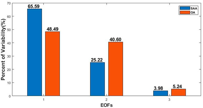
Figure 1. Percentage of variability explained by the first three EOFs obtained from the TIEGCM simulations in the SAA and IO regions.

3 Results and discussion

In this section, the ionospheric MEAN TEC field and the first three modes of variability (EOFi, Ti) in the SAA and IO regions obtained from TIEGCM in 2002 are compared and discussed. Moreover, the correlation coefficient between TEC and Dst is performed in the SAA and IO regions.

3.1 MEAN TEC field

Figure 2A shows the plots of the mean TEC in the SAA region. The MEAN TEC is the result of average treatment to TEC throughout 1 year in the SAA region, and it is the same treatment in the IO region. The most obvious is the peak regions of 100°W to 75W°, which correspond to the peak EIA in South America. It is one of the four peaks of the global EIA distribution. From 100°W to 75°W, the mean TEC presents two maximum area, which are symmetric in general. It can be seen that another maximum area appears near the equator in 30°W to 20°E. Furthermore, the TEC decreases as latitude increases in general. Figure 2B shows the plots of the mean TEC in the IO region. From Figure 2B, there is a maximum distribution of TEC at low latitudes. Besides, TEC shows a change of strength in the latitudinal direction with two peaks at 25°E and 125°E. The maximum areas in Figures 2A, B located in the South America and the Africa, which are parts of the global four-peak structure. Figure 2C shows the diurnal and seasonal variations of TEC in the SAA region in 2002. The ANNUAL TEC is the result of average treatment to TEC throughout whole area in the SAA region, and it is the same treatment in the IO region. From Figure 2C we can see that the mean TEC has significant diurnal variations. Taking the variations in April as an example, the TEC rise at about 5:00LT and reached the maximum at about 14:00LT, and the value of TEC decline at about 16:00LT and reached its minimum at about 3:00LT. In addition, seasonal variations can also be seen. The seasonal variation presents a double-peak structure, with a main peak in August to October, the secondary peak in February to April, a main valley in June and July, and the secondary valley in November and December. Figure 2D shows the diurnal and seasonal variations of TEC in the IO region in 2002. As Figure 2D shows, the TEC in the IO region has similar variations with the SAA region. However, it is noticeable the peaks duration is shorter and the peak intensity is less in the IO region than that in the SAA region.

Figure 2

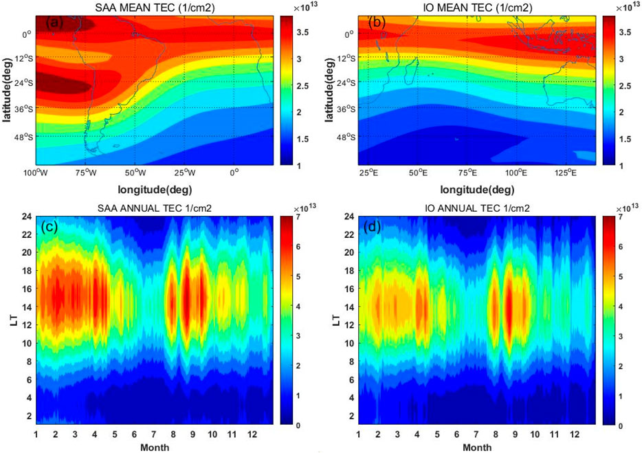
Figure 2. (A) TEC time-averaged maps (1/cm²) derived from the TIEGCM simulations of SAA region. (B) TEC time-averaged maps (1/cm²) derived from the TIEGCM simulations of IO region. (C) The diurnal and seasonal variations of TEC in the SAA region. (D) The diurnal and seasonal variations of TEC in the IO region.

The distributions of MEAN TEC in the SAA and IO regions shown in Figures 2A, B were similar to the result of Oh et al. [7]. Due to the presence of magnetic anomaly in the SAA region, the deviations between geomagnetic and geographic equator produced longitudinal and hemispheric variations in the neutral meridional winds, and then affected EIA distribution [42]. Lin et al. (2017) and [43] suggested that the field-aligned plasma was transported from the summer to winter hemispheres in the morning by neutral winds, and this effect became less around noon. Meanwhile, this created a stronger equatorial fountain effect in the southern hemisphere than that in the northern hemisphere, with more $E\times B$ drift through longitudinally dependent dynamo process occurring south of the equator [44–46]. For the diurnal variations shown in Figures 2C, D, [47] considered that this variation was the result of the equatorial particle fountain (EPF) effect during the day and the $E\times B$ drift velocity during the night. The seasonal variations appeared in the SAA and IO regions, which indicated the TEC was dependent on the seasons. The characteristics were consistent with the results of [21].

3.2 First mode

Figure 3A presents the EOF1 in the SAA regions. The two maximum area are distributed around 100°W, 10°N and 26°S, and the phenomenon of EIA only exists between 100°W and 50°W. The peak regions of 100°W to 75°W still exist, and they distributed on both sides of 12°S, which reflects the symmetrical distribution of EIA in South America. Besides, EOF1 appears to decrease from south to north between 50°W and 20°E. Figure 3B displays the EOF in the IO region. As Figure 3B shows, there is a peak around 135°E and 10°S. Moreover, the EOF decreases from north to south between 100°E and 140°E, and the maximum in the IO region is one peak, which reflects the distribution of EIA in central Pacific. There is a decrease in the zonal direction in EOF1 in the SAA and IO region, which is also consistent with the characteristics in MEAN TEC, and the combined analysis of the two graphs shows that the minimum region of EOF1 is between 25°W and 75°E. As shown in Figures 3C, D, the result of Ti is divided into two dimensions, with the vertical axis representing 24 h and the horizontal axis representing 364 days. The maximum of T1 occurs at 18:00LT, and minimum of T1 occurs at 4:00LT in the SAA region. While the maximum of T1 occurs at 10:00LT, and minimum occurs at 16:00LT in the IO region. For the seasonal variation, T1 is less in June, July and December than in other months in the SAA and IO regions.

Figure 3

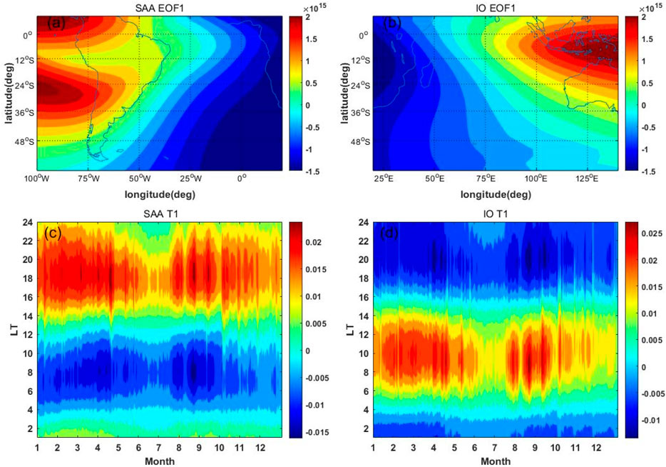
Figure 3. (A) EOF1 derived from the TIEGCM simulations in the SAA region. (B) EOF1 derived from the TIEGCM simulations in the IO region. (C) T1 derived from the TIEGCM simulations in the SAA region. (D) T1 derived from the TIEGCM simulations in the IO region.

Compared with MEAN TEC, EOF1 highlighted the maximums of four-peak structure, the bimodal structure in the SAA region accords with the distribution of EIA, as the research of [44]. The $E\times B$ drift produced the EPF effect with particles settling on both sides of the equator. Besides, this variation in the zonal direction might be related to the change of the lower tide, namely, the dynamo effect in region E [48]. Due to the deviation of the geomagnetic field, the maximum in the SAA region tended to be south of the equator, while the maximum in the IO region occurred near the equator. There were zonal variations of EOF1 in the SAA and IO regions, which had been attributed to variations in tides. [49] thought the tides would act on variations at E-layer because of the heat exchange and radiative absorption, which caused the zonal variation in the SAA and IO regions. In the research of [50], the thermospheric zonal wind also shows a similar variation. Furthermore, the seasonal variation shown in Figures 3C, D was consistent with the study by [21]. However, the T1 maximum occurred at dusk in the SAA region, but at dawn in the IO region. Annual variations in solar activity affected the variations in the ionosphere over 1 year, and the intensity of the EPF effect determines the variation of ionospheric intensity, and the EOF method highlighted it.

3.3 Second mode

Figures 4A, B present the EOF2 in the SAA and IO regions. EOF2 focuses on the peak in Africa and ignores the peak located in South America in the SAA regions, and EOF2 have a single center rather than a bimodal structure like EOF1. It shows decrease from north to south in middle latitude in the SAA region. There is a peak at 10°E around equator in the SAA region, and it exists a decrease from east to west. Besides, the maximum located at 30°E around equator in the IO region, and it exist a decrease from west to east and from north to south. Moreover, the maximum area in the SAA region is smaller than that in the IO region. Figures 4C, D present the T2 in the SAA and IO regions. The maximum of T2 occurs at 11:00LT in the SAA region, and the minimum occurs at 0:00LT, and T2 is less in June and July in the SAA region. The maximum of T2 occurs at 18:00LT in the IO region, and the minimum occurs at 6:00LT, and T2 is also less in June and July.

Figure 4

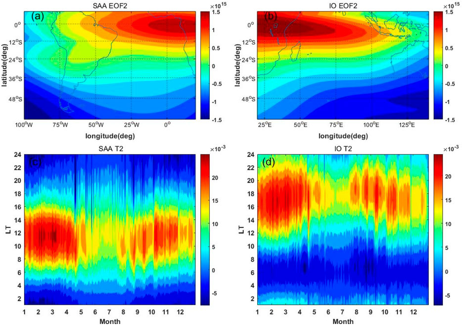
Figure 4. (A) EOF2 derived from the TIEGCM simulations in the SAA region. (B) EOF2 derived from the TIEGCM simulations in the IO region. (C) T2 derived from the TIEGCM simulations in the SAA. (D) T2 derived from the TIEGCM simulations in the IO region.

This EOF mode focused on the peak located in Africa. Consistent with the first mode, the zonal variation was influenced by the lower tides. Moreover, [48] made a comparison between the electron density simulated by TIEGCM and the electron density observed by IMAGE-FUV, which explained the four-peaked longitudinal variation by the effects of an eastward propagating zonal wavenumber-3 diurnal tide (DE3). Besides, the longitudinal variations were relative with solar radiation, and as the latitude increases, the particle deposition decreases. Combined with T1 of the first mode, the maximum of time distribution was mainly at noon and dusk, while the daytime $E\times B$ drift and nighttime downward drift was obvious. Furthermore, the various events of the vertical $E\times B$ drift velocity variations at magnetic equator and the resultant ionospheric featured at low and mid latitudes were researched, [47] revealed the practical consequences of these $E\times B$ events on the equatorial radio signal propagation and the good agreement found with the results of SUPIM. In the second mode, the EOF results showed that the results in the SAA region are more related to the daytime, while the results in the IO region were more related to the nighttime. This result was related to the characteristic of EOF method. When combined with T1, it could be seen that both daytime and nighttime $E\times B$ drift had an impact on Ti in the SAA and IO regions, but the extent of the effect was different. SAA was more affected at dawn, and IO was more affected at dusk.

3.4 Third mode

Figures 5A, B present the EOF3 in the SAA and IO regions. Figure 5A shows EOF3 in the SAA region, and it shows zonal variation in low and middle latitudes. There are two minimum areas, which occur around at 45°W,36°S and 50°W,10°N, and the maximum of EOF3 exist near the low latitudes of 100°W and 20°E. Besides, EOF3 increases from 50°W to 100°W and from 40°W to 20°E. Figure 5B shows EOF3 in the IO region. The minimum is around at 85°E and 10°S, and the maximum is around 23°E and 140°E. The decline of EOF3 from north to south can also be seen in the IO region. Figures 5C, D present the T3 in the SAA and IO regions. Both figures have distinct seasonal and diurnal features. The maximum of T3 occurs around 8:00LT in the SAA region, and the minimum occurs around 18:00LT. The maximum of T3 occurs around 5:00LT in the IO region, and minimum occurs at 15:00LT. There is 3-h lag in the SAA region. Moreover, there are similar characteristic in the SAA and IO regions. The minimum occurs in June and July in the SAA and IO regions, and the dawn-dusk variation appears in both regions.

Figure 5

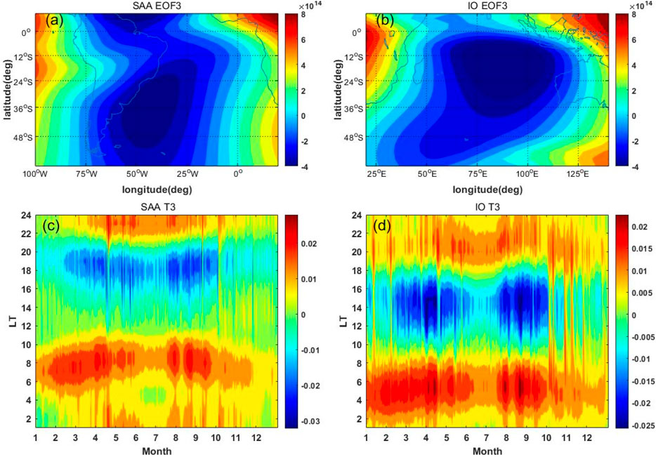
Figure 5. (A) EOF3 derived from the TIEGCM simulations in the SAA region. (B) EOF3 derived from the TIEGCM simulations in the IO region. (C) T3 derived from the TIEGCM simulations in the SAA region. (D) T3 derived from the TIEGCM simulations in the IO region.

As shown in Figures 5A, B, the zonal variations occurred. The maximum areas near 23°E in the two figures corresponded to each other, which could be seen as the four-peak structure is a prominent feature of EIA structure. Although the third mode in the EOF method had a small proportion of variability (3.98% and 5.24%), it still had a clear distribution feature. The maximum were the South America and Africa parts of the four-peak structure. Similar to the first two modes, the solar activity was the main reason for the seasonal variation, and the low tides determined the zonal variation.

3.5 Correlation analysis

Figure 6A shows monthly average TEC in two regions. TEC in the SAA region is higher than that in IO throughout the year particularly from January to April and October to December This might be because there is more particle deposition in the SAA region than that in the IO region [15,16]. Besides, TEC from June to August in the two regions are similar. TEC differ markedly in other months, with less values in the IO region. To compare the influence to ionosphere TEC from geomagnetic field and particle deposition in two regions, the correlation analysis is performed between TEC and Dst. Figure 6B show the hourly TEC in the SAA region and the Dst index during 2002. Figure 6C show the hourly TEC in the IO region and the Dst index during 2002. The correlation coefficient between TEC and Dst is −0.0248 in the SAA region and 0.0534 in the IO region. However, some research show TEC should be related with geomagnetic activities. [51–53], and the result is contrary to expectations. Therefore, there is reason to believe that the TIEGCM is flawed in the impact of geomagnetic activities, and this flaw may be caused by inadequate simulations of the geomagnetic field and particle deposition in the SAA region.

Figure 6

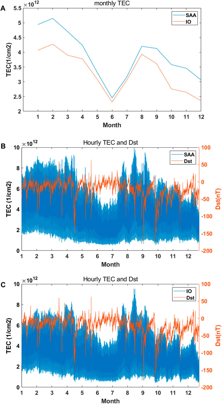
Figure 6. (A) Monthly average TEC in the SAA and IO regions in 2002. (B) Hourly TEC in the SAA region and Dst index in 2002. (C) Hourly TEC in the IO region and Dst index in 2002.

4 Conclusion

In this paper, the ionospheric TEC distribution was simulated by TIEGCM model in the SAA and IO regions in 2002, and EOF method is carried out on these data, and the spatiotemporal variables are separated. The three modes account for 94.7% and 94.3% respectively in the SAA and IO, which represent the basic characteristics of the spatial and temporal characteristic of TEC. In addition, a comparison of TEC between SAA and IO region is performed. Besides, the correlation coefficient between TEC and Dst is done in the SAA and IO regions.

According to the MEAN TEC of the SAA and IO regions, the existence of EIA four-peak structure can be seen. EIA in the SAA region is distributed on both sides of 12°S, while EIA in IO region is distributed on both sides of the equator. Both meridional and zonal variations exist in the MEAN TEC, which may because of the larger magnetic inclination in the SAA region. The first mode accounts for 65.59% and 48.49% of the data variability in the SAA and IO regions respectively. EOF1 reflects the zonal distribution of TEC and the main part of four-peak structure, which is considered to be caused by the difference of geomagnetic field and atmospheric tide, and the enhancement of TEC in SAA region at dusk is emphasized, but the enhancement of TEC in IO region at dawn is emphasized in the first mode. The second mode accounts for 25.22% and 40.60% of the data variability in the SAA and IO regions. EOF2 reflects the zonal and meridian variations, which is closely related to solar radiation and EPF effect. In combination with the two modes, the SAA region is susceptible to the related physical processes during the day, and the IO region is susceptible to the processes at night. The third mode accounts for 3.98% and 5.24% of the data variability in the SAA and IO regions. EOF3 reflects the strong-weak-strong structure of TEC varying with longitude.

As for the temporal variations, the variation of ionospheric TEC shows obvious diurnal and seasonal variations in the SAA and IO regions. TEC value in spring and autumn are lower than those in summer and winter in the southern hemisphere, particularly from January to April and October to December. The EOF methods can separate the dawn-dust variations of TEC. Besides, by comparing the correlation of TEC and Dst between SAA and IO region, we found the difference is not significant. This result indicates that there are some deficiencies in simulation to the specificity of SAA, and the deficiencies are likely caused by the model’s inaccurate simulation of the magnetic field and particle deposition in the SAA region.

Data availability statement

The datasets presented in this study can be found in online repositories. The names of the repository/repositories and accession number(s) can be found in the article/Supplementary Material.

Author contributions

ZL: Conceptualization, Data curation, Funding acquisition, Investigation, Methodology, Project administration, Resources, Supervision, Validation, Writing–review and editing. YW: Conceptualization, Data curation, Formal Analysis, Investigation, Methodology, Software, Visualization, Writing–original draft, Writing–review and editing. JS: Formal Analysis, Writing–review and editing. LW: Formal Analysis, Writing–review and editing. JL: Supervision, Writing–review and editing. HZ: Writing–review and editing. XX: Project administration, Writing–review and editing. CG: Writing–review and editing.

Funding

The author(s) declare that financial support was received for the research, authorship, and/or publication of this article. This research was funded by the National Natural Science Foundation of China (grant numbers 42074183) and the Open Project Program of State Key Laboratory of Lunar and Planetary Sciences (Macau University of Science and Technology) (Macau FDCT grant no. SKL-LPS(MUST)-2021-2023).

Conflict of interest

The authors declare that the research was conducted in the absence of any commercial or financial relationships that could be construed as a potential conflict of interest.

Publisher’s note

All claims expressed in this article are solely those of the authors and do not necessarily represent those of their affiliated organizations, or those of the publisher, the editors and the reviewers. Any product that may be evaluated in this article, or claim that may be made by its manufacturer, is not guaranteed or endorsed by the publisher.

References

1. Forbes JM, Palo SE, Zhang X. Variability of the ionosphere. J Atmos Solar-Terrestrial Phys (2000) 62(8):685–93. doi:10.1016/s1364-6826(00)00029-8

CrossRef Full Text | Google Scholar

2. Clilverd MA, Smith AJ, Thomson NR. The annual variation in quiet time plasmaspheric electron density, determined from whistler mode group delays. Planet Space Sci (1991) 39(7):1059–67. doi:10.1016/0032-0633(91)90113-o

CrossRef Full Text | Google Scholar

3. Rishbeth H, Mendillo M. Patterns of F2-layer variability. J Atmos Solar-Terrestrial Phys (2001) 63(15):1661–80. doi:10.1016/s1364-6826(01)00036-0

CrossRef Full Text | Google Scholar

4. Appleton EV. Two anomalies in the ionosphere. Nature (1946) 157(3995):691. doi:10.1038/157691a0

CrossRef Full Text | Google Scholar

5. Anderson DN. A theoretical study of the ionospheric F region equatorial anomaly—I. Theory. Theory(j) Planet Space Sci (1973) 21(3):409–19. doi:10.1016/0032-0633(73)90040-8

CrossRef Full Text | Google Scholar

6. Balan N, Bailey GJ. Equatorial plasma fountain and its effects: possibility of an additional layer. J Geophys Res (1995) 100(21):21421–32. doi:10.1029/95ja01555

CrossRef Full Text | Google Scholar

7. Oh SJ, Kil H, Kim WT, Paxton LJ, Kim YH. The role of the vertical <I&amp;gt;<B&amp;gt;E&amp;lt;/B&amp;gt;</I&amp;gt;×<I&amp;gt;<B&amp;gt;B&amp;lt;/B&amp;gt;</I&amp;gt; drift for the formation of the longitudinal plasma density structure in the low-latitude F region. Gottingen, Germany: Copernicus Publications (2008) 26(7):2061–7. doi:10.5194/angeo-26-2061-2008

CrossRef Full Text | Google Scholar

8. Mao T, Wan WX, Liu LB. An EOF based empirical model of TEC over wuhan. Chin J Geophys (2005) 48(4):827–34. doi:10.1002/cjg2.720

CrossRef Full Text | Google Scholar

9. Chen Z, Zhang SR, Coster AJ, Fang G. EOF analysis and modeling of GPS TEC climatology over North America. J Geophys Res Space Phys (2015) 120(4):3118–29. doi:10.1002/2014ja020837

CrossRef Full Text | Google Scholar

10. Uwamahoro JC, Habarulema JB. Modelling total electron content during geomagnetic storm conditions using empirical orthogonal functions and neural networks. J Geophys Res Space Phys (2015) 120(12):000–11. doi:10.1002/2015ja021961

CrossRef Full Text | Google Scholar

11. Aa E, Ridley AJ, Huang W, Zou S, Liu S, Coster AJ, et al. An ionosphere specification technique based on data ingestion algorithm and empirical orthogonal function analysis method. Space Weather (2018) 16:1410–23. doi:10.1029/2018SW001987

CrossRef Full Text | Google Scholar

12. Ansari K, Park KD, Panda SK. Empirical Orthogonal Function analysis and modeling of ionospheric TEC over South Korean region. Acta Astronautica (2019) 161:313–24. doi:10.1016/j.actaastro.2019.05.044

CrossRef Full Text | Google Scholar

13. Mandea M, Purucker M. The varying core magnetic field from a space weather perspective(J). Space Sci Rev (2018) 214:1–20. doi:10.1007/s11214-017-0443-8

CrossRef Full Text | Google Scholar

14. Lin CH, Wang W, Hagan ME, Hsiao CC, Immel TJ, Hsu ML, et al. Plausible effect of atmospheric tides on the equatorial ionosphere observed by the FORMOSAT-3/COSMIC: three-dimensional electron density structures. Geophys Res Lett (2007) 34(11). doi:10.1029/2007gl029265

CrossRef Full Text | Google Scholar

15. Domingos J, Jault D, Pais MA, Mandea M. The South atlantic anomaly throughout the solar cycle. Earth Planet Sci Lett (2017) 473:154–63. doi:10.1016/j.epsl.2017.06.004

CrossRef Full Text | Google Scholar

16. Dachev TP. South-atlantic anomaly magnetic storms effects as observed outside the international space station in 2008–2016. J Atmos Solar-Terrestrial Phys (2018) 179:251–60. doi:10.1016/j.jastp.2018.08.009

CrossRef Full Text | Google Scholar

17. Ko CP, Yeh HC. COSMIC/FORMOSAT-3 observations of equatorial F region irregularities in the SAA longitude sector. J Geophys Res Space Phys (2010) 115(A11). doi:10.1029/2010ja015618

CrossRef Full Text | Google Scholar

18. Suvorova AV, Huang CM, Dmitriev AV, Kunitsyn VE, Andreeva ES, Nesterov IA, et al. Effects of ionizing energetic electrons and plasma transport in the ionosphere during the initial phase of the December 2006 magnetic storm. J Geophys Res Space Phys (2016) 121(6):5880–96. doi:10.1002/2016ja022622

CrossRef Full Text | Google Scholar

19. Dmitriev AV, Suvorova AV, Klimenko MV, Ratovsky KG, Rakhmatulin RA, et al. Predictable and unpredictable ionospheric disturbances during St. Patrick's Day magnetic storms of 2013 and 2015 and on 8–9 March 2008. J Geophys Res Space Phys (2017) 122(2):2398–423. doi:10.1002/2016ja023260

CrossRef Full Text | Google Scholar

20. Yi SQ, Xu XJ, Zhou ZL, Chang Q, Wang X, Luo L, et al. Theoretical study of the ionospheric dynamo region inside the South Atlantic Anomaly. Earth Planet Phys (2023) 7(1):84–92. doi:10.26464/epp2023015

CrossRef Full Text | Google Scholar

21. Yu J, Li Z, Wang Y, Shao J, et al. An empirical orthogonal function study of the ionospheric TEC predicted using the TIEGCM model over the South Atlantic anomaly in 2002 and 2008. J Universe (2023) 9(2):102. doi:10.3390/universe9020102

CrossRef Full Text | Google Scholar

22. Roble RG, Ridley EC, Richmond AD, Dickinson RE. A coupled thermosphere/ionosphere general circulation model. Geophys Res Lett (1988) 15(12):1325–8. doi:10.1029/gl015i012p01325

CrossRef Full Text | Google Scholar

23. Richmond AD, Ridley EC, Roble RG. A thermosphere/ionosphere general circulation model with coupled electrodynamics. Geophys Res Lett (1992) 19(6):601–4. doi:10.1029/92gl00401

CrossRef Full Text | Google Scholar

24. Qian L, Burns AG, Emery BA, et al. The NCAR TIE-GCM: a community model of the coupled thermosphere/ionosphere system. Model ionosphere–thermosphere Syst (2014) 73–83. doi:10.1002/9781118704417.ch7

CrossRef Full Text | Google Scholar

25. Chang LC, Lin CH, Liu JY, Balan N, Yue J, Lin J. Seasonal and local time variation of ionospheric migrating tides in 2007–2011 FORMOSAT-3/COSMIC and TIE-GCM total electron content. J Geophys Res Space Phys (2013) 118(5):2545–64. doi:10.1002/jgra.50268

CrossRef Full Text | Google Scholar

26. Maute A, Richmond AD. Examining the magnetic signal due to gravity and plasma pressure gradient current with the TIE-GCM. J Geophys Res Space Phys (2017) 122(12):486–12. doi:10.1002/2017ja024841

CrossRef Full Text | Google Scholar

27. Li Z, Knipp D, Wang W, Sheng C, Qian L, Flynn S. A comparison study of NO cooling between TIMED/SABER measurements and TIEGCM simulations. J Geophys Res Space Phys (2018) 123(10):8714–29. doi:10.1029/2018ja025831

CrossRef Full Text | Google Scholar

28. Li Z, Knipp D, Wang W. Understanding the behaviors of thermospheric nitric oxide cooling during the 15 May 2005 geomagnetic storm. J Geophys Res Space Phys (2019) 124:2113–26. doi:10.1029/2018JA026247

CrossRef Full Text | Google Scholar

29. Li Z, Sun M, Li J, Zhang K, Zhang H, Xu X, et al. Significant variations of thermospheric nitric oxide cooling during the minor geomagnetic storm on 6 may 2015. Universe (2022) 8:236. doi:10.3390/universe8040236

CrossRef Full Text | Google Scholar

30. Rao SS, Chakraborty M, Kumar S, Singh AK. Low-latitude ionospheric response from GPS, IRI and TIE-GCM TEC to solar cycle 24. Astrophysics Space Sci (2019) 364:216–4. doi:10.1007/s10509-019-3701-2

CrossRef Full Text | Google Scholar

31. Zhang KD, Wang H, Wang WB, Liu J, Zhang S, Sheng C. Nighttime meridional neutral wind responses to SAPS simulated by the TIEGCM: a universal time effect. Earth Planet Phys (2021) 5(1):1–11. doi:10.26464/epp2021004

CrossRef Full Text | Google Scholar

32. Wang H, Lühr H, Zhang KD. Longitudinal variation in the thermospheric superrotation: CHAMP observation and TIE-GCM simulation. Geophys Res Lett (2021) 48(18):e2021GL095439. doi:10.1029/2021gl095439

CrossRef Full Text | Google Scholar

33. Björnsson H, Venegas SA. A manual for EOF and SVD analyses of climatic data. CCGCR Rep (1997) 97(1):112–34.

Google Scholar

34. Wilks DS. Principal component (EOF) analysis. Int Geophys (2011) 100:519–62. Academic Press. doi:10.1016/b978-0-12-385022-5.00012-9

CrossRef Full Text | Google Scholar

35. Bro R, Smilde AK. Principal component analysis. Anal Methods (2014) 6(9):2812–31. doi:10.1039/c3ay41907j

CrossRef Full Text | Google Scholar

36. Ding YG, Liang JY, Liu JF. New research on diagnoses of meteorological variable fields using EOF/PCA(J). Chin J Atmos Sci (2005) 29(2):307–13.

Google Scholar

37. Lei J, Dou X, Burns A, Wang W, Luan X, Zeng Z, et al. Annual asymmetry in thermospheric density: observations and simulations. J Geophys Res Space Phys (2013) 118(5):2503–10. doi:10.1002/jgra.50253

CrossRef Full Text | Google Scholar

38. Talaat ER, Zhu X. Spatial and temporal variation of total electron content as revealed by principal component analysis. Gottingen, Germany: Copernicus Publications (2016) 34(12):1109–17. doi:10.5194/angeo-34-1109-2016

CrossRef Full Text | Google Scholar

39. Ruan H, Lei J, Dou X, Liu S, Aa E. An exospheric temperature model based on CHAMP observations and TIEGCM simulations. Space Weather (2018) 16(2):147–56. doi:10.1002/2017sw001759

CrossRef Full Text | Google Scholar

40. Flynn S, Knipp DJ, Matsuo T, Mlynczak M, Hunt L. Understanding the global variability in thermospheric nitric oxide flux using empirical orthogonal functions (EOFs). J Geophys Res Space Phys (2018) 123(5):4150–70. doi:10.1029/2018ja025353

CrossRef Full Text | Google Scholar

41. Li Z, Knipp D, Wang W, Shi Y, Wang M, Su Y, et al. An EOFs study of thermospheric nitric oxide flux based on TIEGCM simulations. J Geophys Res Space Phys (2019) 124(11):9695–708. doi:10.1029/2019ja027004

CrossRef Full Text | Google Scholar

42. Balan N, Rajesh PK, Sripathi S, Tulasiram S, Liu J, Bailey G. Modeling and observations of the north–south ionospheric asymmetry at low latitudes at long deep solar minimum. Adv Space Res (2013) 52(3):375–82. doi:10.1016/j.asr.2013.04.003

CrossRef Full Text | Google Scholar

43. Tulasi Ram S, Su SY, Liu CH. FORMOSAT-3/COSMIC observations of seasonal and longitudinal variations of equatorial ionization anomaly and its interhemispheric asymmetry during the solar minimum period. J Geophys Res Space Phys (2009) 114(A6). doi:10.1029/2008ja013880

CrossRef Full Text | Google Scholar

44. Deminov MG, Kochenova NA, Sitnov YS. Longitudinal variations of the electric field in the dayside equatorial ionosphere. Geomagn Aeron (1988) 28:57–60.

Google Scholar

45. Batista IS, De Medeiros RT, Abdu MA, de Souza JR, Bailey GJ, de Paula ER. Equatorial ionospheric vertical plasma drift model over the Brazilian region. J Geophys Res Space Phys (1996) 101(A5):10887–92. doi:10.1029/95ja03833

CrossRef Full Text | Google Scholar

46. Ren Z, Wan W, Liu L, Heelis RA, Zhao B, Wei Y, et al. Influences of geomagnetic fields on longitudinal variations of vertical plasma drifts in the presunset equatorial topside ionosphere. J Geophys Res Space Phys (2009) 114(A3). doi:10.1029/2008ja013675

CrossRef Full Text | Google Scholar

47. Horvath I, Essex EA. Vertical <i&amp;gt;E&amp;lt;/i&amp;gt; × <i&amp;gt;B&amp;lt;/i&amp;gt; drift velocity variations and associated low-latitude ionospheric irregularities investigated with the TOPEX and GPS satellite data. Gottingen, Germany: Copernicus Publications (2003) 21(4):1017–30. doi:10.5194/angeo-21-1017-2003

CrossRef Full Text | Google Scholar

48. Hagan ME, Maute A, Roble RG, Richmond AD, Immel TJ, England SL. Connections between deep tropical clouds and the Earth's ionosphere. Geophys Res Lett (2007) 34(20). doi:10.1029/2007gl030142

CrossRef Full Text | Google Scholar

49. Hagan ME, Forbes JM. Migrating and nonmigrating diurnal tides in the middle and upper atmosphere excited by tropospheric latent heat release. J Geophys Res Atmospheres (2002) 107(D24). ACL 6-1-ACL 6-15. doi:10.1029/2001jd001236

CrossRef Full Text | Google Scholar

50. Zhang K, Wang W, Wang H, Dang T, Liu J, Wu Q. The longitudinal variations of upper thermospheric zonal winds observed by the CHAMP satellite at low and midlatitudes. J Geophys Res Space Phys (2018) 123(11):9652–68. doi:10.1029/2018ja025463

CrossRef Full Text | Google Scholar

51. Sergeeva MA, Maltseva OA, Gonzalez-Esparza JA, Mejia-Ambriz JC, De la Luz V, Corona-Romero P, et al. TEC behavior over the Mexican region. Ann Geophys (2018) 61(1):GM104. doi:10.4401/ag-7465

CrossRef Full Text | Google Scholar

52. Sunardi B, Muslim B, Sakya AE, Rohadi S, Sulastri S, Murjaya J. Ionospheric earthquake effects detection based on total electron content (TEC) GPS correlation[C]//IOP conference series: Earth and environmental science. IOP Publishing (2018) 132(1):012014. doi:10.1088/1755-1315/132/1/012014

CrossRef Full Text | Google Scholar

53. Zhang K, Wang H, Yamazaki Y. Effects of subauroral polarization streams on the equatorial electrojet during the geomagnetic storm on 1 June 2013: 2. The temporal variations. J Geophys Res Space Phys (2022) 127(2):e2021JA030180. doi:10.1029/2021ja030180

CrossRef Full Text | Google Scholar