Spin glass dynamics through the lens of the coherence length

1 Introduction

The dynamical processes found in spin glasses mimic those from a wide variety of physical systems, not limited to glass formers, polymers, granular materials, phase separation in the early Universe, and the social sciences. Because their dynamical properties can be measured directly, they provide a window into the behavior of far-from-equilibrium systems. This review will explore the spin glass coherence length, ξ(t, t_w; H), its definition, extraction from experiment and simulations, and applications. Here, t_w is the age of the spin glass system before the measurement time, t begins, and H is the magnetic field. An inherent advantage of the use of ξ(t, t_w; H) to describe dynamical properties is that the spin glass transition temperature, T_g is implicit. A precise value of T_g is not required even for explorations close to T_g.

The first explicit experimental procedure for extraction of the spin glass was proposed and demonstrated by Joh et al. [1]. They noted that the relevant free energy barrier energy change from imposition of a magnetic field H was given by what they termed the “Zeeman” energy, E_Z where,

$E_Z=N_s{\chi }_{\text{FC}}{H}^2.(1)$

Here, N_s is the number of spins in a volume subtended by ξ(t, t_w; H), and χ_FC is the field-cooled susceptibility per spin. They took $N_s=(4/3)\pi {[\xi (t,t_w;H)]}^3$ whereas, subsequently, a value based on the structure of the four spin coherence length was introduced [2],

$N_s={\left[\xi \left(t,t_w;H\right)\right]}^{D-\left(\theta /2\right)}(2)$

where θ is the replicon exponent [3].

The Sherrington-Kirpatrick (SK) infinite range exchange Hamiltonian [4] for spin glasses exhibits states within an ultrametric geometry [5] which has a pictorial equivalent [6] of an hierarchical organization. Free energy barriers separate states with occupancies that increase exponentially with diminishing overlap. The Parisi solution [7, 8] of the SK model are “pure states” separated by infinite barriers. This geometry was shown by analogy to replicate dynamical transitions between states with finite free energy barriers [9]. Putting all these factors together leads to an inflection point in the time dependence of the magnetization, and hence a maximum in the logarithmic derivative of the time dependent magnetization, known as S (t, t_w; H), the relaxation function:

$S\left(t,t_w;H\right)=\frac{dM\left(t,t_w;H\right)}{dlnt}.(3)$

Experimentally, the magnetization is measured at constant temperature T after an aging time t_w. Empirically, the maximum of S (t, t_w; H) occurs at a time t ≈ t_w [10] associated with the largest free energy barrier generated by the growth of the spin glass coherence length ξ(t, t_w; H) where H is the magnetic field.

In a thermoremanent magnetization (TRM) experiment, H is applied in the paramagnetic state, kept constant as the spin glass is cooled to a temperature T below the condensation temperature T_g, and the magnetization is measured after the time t_w when H is changed (most often, cut to zero). In a zero-field cooled (ZFC) experiment, H = 0 initially as the spin glass is cooled to T, and the magnetization measured upon application of H after the time t_w. It is important to understand that the free energy barriers are not “chemical” in their origin. Rather, they are created by larger and larger numbers of correlated spins, the volume containing N_s subtended by ξ(t, t_w; H) according to Eq. 2.

Thus, the maximum free energy barrier height, Δ_max is associated with t_w according to an Arrhenius law,

${\mathrm{\Delta }}_{\text{max}}\approx k_{\text{B}}Tln\left[\frac{t_w}{{\tau }_0}\right](4)$

where τ₀ is an exchange time usually taken as ℏ/k_BT_g. From Eq. 1, we can define an “effective” waiting time $t_w^{\text{eff}}$ in the presence of a magnetic field as,

${\mathrm{\Delta }}_{\text{max}}-N_s{\chi }_{\text{FC}}{H}^2=k_{\text{B}}Tln{t}_w^{\text{eff}}-k_{\text{B}}Tln{\tau }_0,(5)$

where $t_w^{\text{eff}}$ is taken as the time when S (t, t_w; H) reaches its peak in the absence/presence of H for TRM/ZFC experiments, respectively.

Combining Eqs 1, 5 enables the only means for extraction of the spin glass coherence length from experiment. In order to keep this value explicit, we shall label it ξ_Zeeman.

Mathematical simulations from the Janus Collaboration [11], using a special purpose computer, can address the value of ξ directly. In temperature cycling experiments that will be addressed below, they project (at least) two different coherence lengths [12].

The first is ξ_micro (t_w, T), the microscopic coherence length computed directly from the replicon propagator [13, 14] in Eq. 6

${\mathcal{G}}_{\text{R}}\left(\mathbf{r},t,T\right)=\frac{1}{V}\sum _{\mathbf{x}}\stackrel{̄}{{\left({⟨s_{\text{x},t}{s}_{\mathbf{x}+\mathbf{r},t}⟩}_T-{⟨s_{\mathbf{x},t}⟩}_T{⟨s_{\mathbf{x}+\mathbf{r},t}⟩}_T\right)}^2},(6)$

where for Ising spins, s_x = ±1. The replicon correlator ${\mathcal{G}}_{\text{R}}$ decays to zero in the long-distance limit. One therefore computes ξ_micro (t_w, H) by exploiting the integral estimators [15, 16] in Eqs 7 and 8

$I_k\left(t,T\right)={\int }_0^{\infty }dr{r}^k\mathcal{G}\left(\mathbf{r},t;T\right),(7)$

and

${\xi }_{k,k+1}\left(t,T\right)=\frac{I_{k+1}\left(t,T\right)}{I_k\left(t,T\right)}.(8)$

The ξ_1,2 (t_w, T) is designated as the microscopic coherence length ξ_micro (t_w, T).

Physically [12], “ξ_micro (t_w, T) is the size of the (glassy) domains within the sample (it is the largest length scale at which we can regard the system as ordered at time t_w.”

Another length scale is introduced in simulations [12] when comparing the same system at two times t₁ and t₂ (t₁ < t₂): ζ(t₁, t₂). It “characterizes the long-distance decay of the pair-correlation function corresponding to the set of spins taking opposite signs at times t₁ and t₂. Physically, ζ(t₁, t₂) is the typical size of regions where coherent rearrangements have occurred between times t₁ and t₂ … because of the ongoing formation of a new spin order at time t₂. For fixed t₁, ζ(t₁, t₂) grows with t₂ starting from ζ(t₁, t₂ = t₁) = 0.”

At a given temperature, ξ_Zeeman (t_w, T) “fairly closely follows the behavior of the microscopic length ξ_micro (t_w, T)” [12, 17–19] so that, for all practical purposes, they can be taken equal. For varying temperature protocols, the scenario is more intricate because of the presence of temperature chaos at large temperature changes. The length scales are quantitatively compared in Figure 5 of [18].

Now that we have defined the relevant length scales, we show in the next section how they elucidate the dynamical properties of spin glasses.

2 Physical properties

The first experimental extraction of ξ_Zeeman (t_w, T) [1] compared results from two approaches: power law dynamics [20] vs. activated dynamics [21]. The results are reproduced in Figure 1. Knowing χ_FC per spin from other measurements allows for the extraction of ξ_Zeeman (t_w, T) from Eq. 2. For example, from Figure 1 at t_w = 1, 000 s, N_s ≈ 3 × 10⁶ spins. They set $\xi (t_w,T)\approx {[N_s(t_w,T)]}^{1/3}$ giving ξ(t_w = 1, 000, T = 28 K) = 100 a₀, where a₀ is the average distance between Mn ions. Subsequently it was shown [3] that the correct extraction of ξ(t_w, T) is given by ${[N_s(t_w,T)]}^{1/d_f}$, where d_f is the fractal dimension equal to D − (θ/2), with θ the replicon exponent [16]. In general, θ ∼ 0.3–0.4 so that its omission in Ref. [1] results in only a small error.

Figure 1

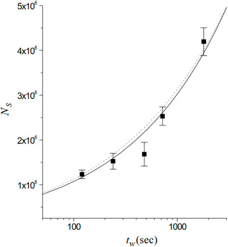
Figure 1. A plot of N_s reproduced from [1] for CuMn 6 al.% vs. t_w on a log scale at fixed temperature T = 0.89 T_g = 28 K. The solid curve drawn through the points is the prediction for power law dynamics [20], while the dashed curve is the prediction for activated dynamics [21], with their exchange factor set equal to T_g (i.e., independent of T and t). As is seen from the two curves, the two fits are equally good.

The uses of ξ(t_w, T) to describe physical processes provides a powerful quantitative tool. Pertinent examples are described below.

2.1 Slowing down of the growth of ξ(t_w, T)

The Janus Collaboration utilizes a special purpose-built computer [16] to examine the dynamics of the Ising spin glass. They were able to explore the (re-normalized) aging rate [22],

$z_c\left(T,\xi \right)=\frac{T}{T_g}\frac{dln{t}_w}{dln\xi }.(9)$

The re-normalizing factor T/T_g makes z_c (T, ξ) ≈ z_c(ξ) [23].

We can rewrite Eq. 9 as Eq. 10,

$ln{t}_w=\frac{z_c{T}_g}{T}ln\xi +\text{const}(10)$

The aging rate, z_c, was found to vary substantially from experiment to experiments, depending upon the temperature and nature of the spin glass sample. For example, for a bulk polycrystalline sample of CuMn (6 at%) [1] found z_c = 5.917 at a reduced temperature of T/T_g = 0.89. For a polycrystalline bulk spinel they found z_c = 7.576 at a reduced temperature of T/T_g = 0.72.

In thin films [24] found for 11.7 at. % that z_c = 9.62 at reduced temperatures of T/T_g = 0.43, 0.59, and 0.78. Working at T/T_g = 0.95 [25], found z_c = 6.80 in bulk polycrystalline CuMn (5 at%).

The Janus collaboration [22] found a hint to reconcile these apparently conflicting values from experiment by computing ξ over a temperature range 0.5 ≤ T/T_g ≤ 1. Figure 2 exhibits their results.

Figure 2

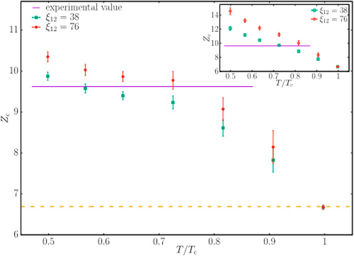
Figure 2. Value of the experimental aging rate for spin glasses Z_c(T) = z_c (T, ξ)T/T_c, reproduced from Ref. [22]. The straight line is the experimental value of z_c(T) ≈ 9.62 from Ref. [23].

Experimentally, there is a significant confirmation for this variation of z_c. Ref. [22] found that the growth of ξ(t_w, T) slows down as ξ(t_w, T) increases. That is, z_c increases as ξ(t_w, T) increases. In order to achieve large values of ξ(t_w, T) to test this simulation prediction, we were blessed with a single crystal of CuMn, 6 at%, grown by Dr. D.L.Schagel, the description of which is contained in Ref. [26]. By working at 28 K (T_g = 31.5 K) and at long waiting times (up to 10₅ s), the value extracted for ξ(t_w, T) reached 150 nm, the largest coherence length ever reported for a glassy system [26]. The value of ξ(t_w, T) vs. t_w is plotted in Figure 3, from which z_c = 12.37 ± 1.07 can be extracted. This is to be compared with z_c ≈ 9.62 extracted at shorter waiting times for smaller values of ξ(t_w, T).

Figure 3

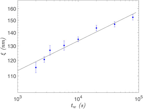
Figure 3. ξ(t_w, T) as a function of the waiting time t_w at a measuring temperature of T = 28 K (T_g = 31.5 K) reproduced from Ref. [26]. The staight line is a fit to ln t_w = (z_cT_g/T) ln ξ + const. [recall Eq. 10], yielding Z_c = 12.37 ± 1.07.

2.2 Scaling law

The coherence length ξ(t_w, T) can be measured precisely for spin glasses both in experiment and through simulations. However, known analysis methods lead to discrepancies either for large external magnetic fields or close to the transition temperature. This problem can be solved through introduction of a scaling law that takes into account both the magnetic field and the time-dependent coherence length. This is especially important because temperatures T ≈ T_g are most relevant for the study of glass formers (ξ is restricted to a very narrow window of variation if one moves away from T_g).

Historically, non-linear magnetization effects, and their scaling properties in spin glasses, were first introduced by Malozemoff, Barbara, and Imry [27–29] who introduced the relation for the singular part of the magnetic susceptibility,

${\chi }_s=H^{2/\delta }f\left(t_r/H^{2/\varphi }\right),(11)$

where f(x) is a constant for x → 0; f(x) = x^−γ for x → ∞; ϕ = γδ/(δ − 1) ≡ βδ; and t_r is the reduced temperature T/T_g.

This form was used by Lévy and Ogielski [30], and Lévy [31] who measured the AC non-linear susceptibilities of very dilute AgMn alloys above and below T_g as a function of frequency, temperature, and magnetic field. Their critical exponents from Eq. 11 differed substantially from Monte Carlo simulations for short-range Ising systems [32]. The discrepancy in their value of γ was very large, and most probably arose from the lack of an exact value for T_g in their experiments. This illustrates the value of and need for a different approach for scaling the non-linear magnetization of spin glasses in the vicinity of T_g.

The scaling argument goes as follows. Let M(t, t_w; H) be the magnetization per spin. The generalized susceptibilities χ₁, χ₃, χ₅, … are defined through the Taylor expansion,

$M\left(H\right)={\chi }_{1}H+\frac{{\chi }_3}{3!}{H}^3+\frac{{\chi }_5}{5!}{H}^5+\mathcal{O}\left(H^7\right).(12)$

We have omitted t and t_w for brevity. Our hypothesis is that, in the non-equilibrium regime for a spin glass close to T_g in the presence of a small magnetic field,

$\begin{array}{c}\hfill M\left(t,t_w;H\right)={\left[\xi \left(t+t_w\right)\right]}^{y_H-D}\\ \hfill \times \mathcal{F}\left(H{\left[\xi \left(t+t_w\right)\right]}^{y_H},\frac{\xi \left(t+t_w\right)}{\xi \left(t_w\right)}\right)\end{array}(13)$

According to full-aging spin-glass dynamics [30] Eq. 13 tells us that ξ(t + t_w)/ξ(t_w) will be approximately constant close to the maximum of the relaxation rate [i.e., peak of S(t)], so that we omit this dependence. Thus, combining Eqs 12, 13, one can express the generalized susceptibilities χ₁, χ₃, χ₅, … in terms of the spin glass coherence length ξ(t, t_w; H):

${\chi }_{2n-1}\propto |\xi \left(t_w\right){|}^{2n{y}_H-D},(14)$

where we have omitted the arguments t and H for convenience, and Eq. 15

$2y_H=D-\frac{\theta \left(\bar{x}\right)}{2},(15)$

with $\theta (\bar{x})$ the replicon exponent [3].

The first term of M(H) in Eq. 12 is χ₁, which contains the linear term as well as the first non-linear scaling term, so that we write,

${\chi }_1=\frac{\widehat{S}}{T}+\frac{a_1\left(T\right)}{{\xi }^{\theta \left(\bar{x}\right)/2}}(16)$

where a₁(T) is some unknown constant, hopefully varying smoothly with temperature.

The free-energy variation per spin in the presence of a magnetic field can be derived by integrating the magnetic density Eq. 12 with respect to the magnetic field in Eq. 17,

$\mathrm{\Delta }F=-\left[\frac{{\chi }_1}{2}{H}^2+\frac{{\chi }_3}{4!}{H}^4+\frac{{\chi }_5}{6!}{H}^6+\mathcal{O}\left(H^8\right)\right].(17)$

Substituting the scaling from Eqs 14, 16, the free energy ΔF can be written as (we drop the $\bar{x}$ dependence of θ for brevity) in Eq. 18,

$\begin{array}{c}\hfill \mathrm{\Delta }F=-\left[\frac{\widehat{S}}{2T}{H}^2+\frac{a_1\left(T\right)}{{\xi }^{\theta /2}}{H}^2+a_3\left(T\right){\xi }^{D-\theta }{H}^4\right.\\ \hfill \left.+a_5\left(T\right){\xi }^{2D-\left(3\theta /2\right)}{H}^6+\mathcal{O}\left(H^8\right)\right],\end{array}(18)$

where again the a_n(T) are unknowns and hopefully again smoothly varying functions of temperature. Using the effective response time, $t_H^{\text{eff}}$, to reflect the total free-energy change at magnetic field H with respect to H → 0⁺,

$\begin{array}{c}\hfill ln\left[\frac{t_H^{\text{eff}}}{t_{H\to 0^{+}}^{\text{eff}}}\right]=N_s\mathrm{\Delta }F\\ \hfill =-b\left[\left(\frac{\widehat{S}}{2T}+\frac{a_1\left(T\right)}{{\xi }^{\theta /2}}\right){\xi }^{D-\left(\theta /2\right)}{H}^2\right]\\ \hfill \left.+a_3\left(T\right){\xi }^{2D-\left(3\theta /2\right)}{H}^4+a_5\left(T\right){\xi }^{3D-2\theta }{H}^6+\mathcal{O}\left(H^8\right)\right]\end{array}(19)$

where the coefficient b is a geometrical factor, and we have absorbed the k_BT term in the a_n(T) coefficients. The correction term $a_1(T)/{\xi }^{\theta (\tilde{x})/2}$ is small compared to $\widehat{S}/T$, so it will be neglected in subsequent expressions. Equation 19 shows that the higher order terms have the functional form, in Eq. 20,

${\chi }_{2n-1}\frac{H^{2n}}{\left(2n\right)!}=a_{2n-1}\left(T\right){\xi }^{-\theta \left(\tilde{x}\right)/2}{\left[{\xi }^{2y_H}{H}^2\right]}^n(20)$

where, in Eq. 21

$2y_H=D-\frac{\theta \left(\tilde{x}\right)}{2}(21)$

This leads to the new scaling relation,

$ln\left(\frac{t_H^{\text{eff}}}{t_{H\to O^{+}}^{\text{eff}}}\right)=\left.\frac{\widehat{S}}{T}{\xi }^{D-\left(\theta /2\right)}{H}^2+{\xi }^{-\theta /2}\mathcal{G}\left({\xi }^{D-\left(\theta /2\right)}{H}^2;T\right)\right).(22)$

where the geometrical factor b has been absorbed into the scaling function $\mathcal{G}$).

Among the many uses of Eq. 22, two can be highlighted. The first is the issue surrounding the magnetization encompassed in ξ_Zeeman (t_w, T). The original introduction proposal, Ref. [1], envisaged the reduction of the barrier heights Δ(t_w, T) by E_Z [Eq. 1] to be caused by the magnetization induced by the magnetic field within the volume subtended by the spin glass coherence length ξ(t_w, T), viz Eq. 1. A subsequent treatment [33] associated E_Z with the magnetization associated with the fluctuations of the entire system of N spins, namely, $\propto \sqrt{N}$. The magnetic field dependence is very different, the former E_z ∝ H² while the latter E_Z ∝ H.

A comparison of the two was exhibited in Fig. 10 of Ref. [17], reproduced here as Figure 4. The magnitude of the magnetic fields contained in Figure 4 are quite large. The authors of Ref. [33] state that the proportionality to H fails at low magnetic fields. The reader can judge whether a linear fit to H is obeyed by the left-hand of Figure 4. The right-hand of Figure 4 is the fit to the scaling law, valid over the full range of H, large and small. Again, the reader can judge which fit is preferable.

Figure 4

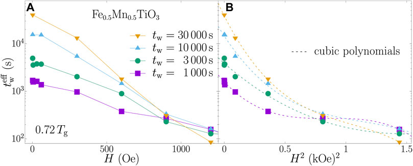
Figure 4. (A) Effective waiting times (log scale) derived from field-change experiments on an Ising sample (Fe_0.5Mn_0.5TiO₃) as a function of magnetic field H. The plot reproduces Figure 10 of Paga et al. [17] (solid lines are linear interpolations to data with the same t_w). (B) The same data plotted against H². The dotted lines are fits to Eq. 19.

The second is the value of the condensation temperature, T_g. In principle, determination of T_g would require an infinite t_w because ξ(T) → ∞ when T → T_g. One expects that any experiment at finite t_w would yield a maximum for the non-linear susceptibility at a temperature we shall call T_g (t_w) because t_w is finite.

In principle then, by measuring T_g (t_w) for ever larger t_w, one could extrapolate to the true t_w → ∞ condensation temperature T_g. If nothing else, measurements at large values of t_w on laboratory time scales could establish an upper bound for T_g.

The non-linear susceptibility χ₃ diverges as Eq. 23

${\chi }_3\left(t_w\to \infty ;T\right)={\chi }_0\frac{T_g\left(t_w\to \infty \right)}{|T_g\left(t_w\to \infty \right)-T{|}^{\gamma }},(23)$

where χ₀ is a constant independent of temperature, and γ = 6.13 (11) from Ref. [32]. For finite t_W, χ₃ (t_w, T) only has a maximum as a function of temperature. A way of arriving at this maximum would be to fit the data to the function, in Eq. 24

${\chi }_3\left(t_w,T\right)={\chi }_0\frac{T_g\left(t_w\right)}{|T_g\left(t_w\right)-T{|}^{\gamma }},(24)$

and then use data points from just two or three temperatures to extract T_g (t_w). For larger and larger t_w, one could in principle extrapolate to the true T_g. This is just a suggestion for a feasible process for taking laboratory data for finite t_w and extrapolating to find T_g (t_w → ∞).

2.3 Temperature chaos

Temperature chaos is one of the outstanding mysteries posed by spin glasses. It consists of the complete reorganization of the equilibrium configurations by the slighted change in temperature.” [34] These are the opening lines of a major paper titled “Temperature chaos is a non-local effect” and set the stage for this section. Even the existence of temperature chaos in spin glasses has been questioned [35–38]. Recent experiments [39] and simulations [40] have shed light on its existence and nature, but there are many questions that remain.

From this article’s perspective, the opening gambit was the renormalization group perspective of Bray and Moore [41]. They introduced a length scale associated with temperature chaos that, for all practical purposes, can be simplified to,

${\ell }_c\left(T_1,T_2\right)=a_0{\left[\frac{T_2}{T_1-T_2}\right]}^{1/\zeta }(25)$

where ζ = d_s − θ, d_s the fractal dimension of the correlated region, and θ is the replicon exponent. The system is in an equilibrium state at a temperature T₁, after which the temperature is dropped to T₂. Temperature chaos obtains with a length scale ℓ_c. The reason that ℓ_c is important is that, for a coherence length ξ(t_w, T) not infinite, temperature chaos requires a finite temperature drop. The condiction is, shown in Eq. 26

$\begin{array}{c}\hfill \text{Temperature\hspace{0.17em}chaos}:{\ell }_c\left(T_1,T_2\right)\le \xi \left(t_w,T_1\right),\\ \hfill \text{Reversible}:{\ell }_c\left(T_1,T_2\right)\ge \xi \left(t_w,T_1\right),\end{array}(26)$

where by “reversible” we mean that the system “remembers where it came from” when the temperature is dropped from T₁ to T₂, i.e., no temperature chaos.

Though the relationship Eq. 25 is for a spin glass in equilibrium, realistically, this is never the case. Fortunately, recently an analysis was provided [40] which is titled “Temperature chaos is present in off-equilibrium spin-glass dynamics,” so that we can use the relationship Eq. 25 experimentally. Note that both t_w and ΔT = T₁ − T₂ are controllable parameters. Hence, we can probe the onset of temperature chaos by examining spin glass dynamics under difference conditions, and in particular, can control its onset.

Experiments have probed temperature chaos. The first definitive paper [42] defined the length scale for chaos as L_ΔT given by Eq. 27,

$L_{\mathrm{\Delta }T}\sim L_0|\mathrm{\Delta }T/J{|}^{-1/\zeta }(27)$

equivalent to our Eq. 25 with L_ΔT ≡ ℓ_c (T₁, T₂), and J an exchange energy in units of temperature. They extract and effective chaos length scale, L_eff from the following plot (their Figure 4, our Figure 5): Their plot generates 1/ζ = 2.6 or ζ = 0.38. This value is a factor of nearly 3 below the rather universally accepted value of ζ = 1.1 (see Appendix B in Ref. [39], for a full listing of theoretical values for ζ).

Figure 5

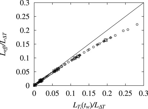
Figure 5. Reproduced from Figure 4 in [42]. Scaling plot of L_eff with L_ΔT = L₀ (cΔT/J)^−2.6 with c = 5. The solid straight line represents scaling in the absence of temperature chaos.

It is difficult to understand why their value for ζ was so far off from what is now regarded as the fairly accepted value near unity. An origin may be lie in their measurement protocol, namely, a zero-field magnetization measurement where the magnetic field is applied after cycling to T₁. Magnetic field chaos [43, 44] could then be compounded with temperature chaos, and distort the extraction of a value for 1/ζ.

In order to circumvent this possibility, Zhai et al. [39] worked with a protocol where the magnetic field remained constant across temperature cycling. The idea was to use the field-cooled magnetization to investigate temperature chaos in spin glasses. This protocol involved turning on a magnetic field H above the condensation temperature, T_g, keeping it constant throughout the temperature cycling protocol.

The specific steps were as follows. The decay of the field cooled (FC) magnetization, M_FC(t, T₁, H) is measured at the first temperature stop T₁ after cooling in the current magnetic field and waiting a time t_w1. The decay curve is denoted as the “reference curve.” Then, temperature cycling is engaged, where one first cools to temperature T₁, waits a time t_w1, cools to T₂, waits a time t_w2, then rapidly warms back to T₁, and measures the decay of the magnetization M_FC(t, T₁, H).

In order to observe TC, T₁ was fixed and the temperature T₂ was gradually lowered in separate experimental runs to T₂ = T₁ − ΔT. Following the temperature drop, if,

$x=\frac{{\ell }_c\left(T_1,T_2\right)}{\xi \left(T_1,t_{w1}\right)}\ge 1,(28)$

the coherence length will continue to grow, and one remains in the reversible state. However, in Eq. 29

$x=\frac{{\ell }_c\left(T_1,T_2\right)}{\xi \left(T_1,t_{w1}\right)}\le 1(29)$

temperature chaos sets in and one finds a diminished coherence length after heating back to temperature T₁ (see the discussion below of memory).

As a consequence, under reversible dynamics, Eq. 28, the decay curve of M_FC(t, T₁, H) after temperature cycling can be superposed on the reference decay curve, allowing for a positive shift in time for M_FC(t, T₁, H) during the time that T < T₁. However, after the onset of temperature chaos, The decay curves cannot be superposed for any positive shift of M_FC(t, T₁, H) in time.

This is seen explicitly in Figure 6 which was reproduced from Figure 1 of Ref [39]. By changing T₁, t_w1, Eq. 25 can be probed to yield a value for 1/ζ. A value for ζ ≈ 1.1 was extracted in [39], very close to a majority of the theoretical values.

Figure 6

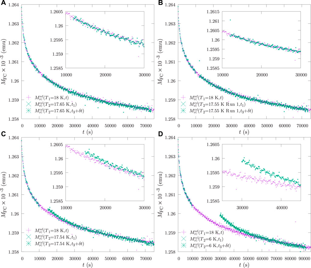
Figure 6. The example of T₁ = 18 K, reproduced from Figure 1 in [39]. The temperature is gradually lowered to T₂ after t_w1 = 10⁴ s and heated back to T₁ after t_w2 = 10³ s. The temperature cycling curve is then shifted by δt to overlap the reference curve. In the reversible temperature range, (A) and (B), the cycling curve can be overlapped with the reference curve over the whole period $\approx 7\times 10^4$ s. In the chaotic range, (C) and (D), the cycling curve can only be partially overlapped. Hence, temperature chaos, at T₁ = 18 K, t_w1 = 10⁴ s, sets in for ΔT > 450 mK.

This experimental evidence for the existence of temperature chaos in spin glasses will prove important in our subsequent treatments of rejuvenation and memory. We shall argue that temperature chaos is responsible for the former, and plays an important role in a quantitative treatment of the latter. In any case, the experiments of Ref. [34] have shown that temperature chaos is present in spin glasses, and will be shown to have a profound impact in other dynamical spin glass phenomena.

2.4 Rejuvenation

The singular publication that engendered the attention of both theorists and experimentalists for over three decades was that of Jonason et al. [45] titled “Memory and Chaos Effects in Spin Glasses.” They displayed the remarkable figure (Figure 7 reproduced from Figure 1 in their paper). The system is “aged” at 12 K, becoming “older.” Upon lowering the temperature, it returns to the reference curve, thus becoming “younger”. This is termed “rejuvenation.” It was attributed to temperature chaos, namely, the spin glass “forgot” its previous history of aging when the temperature was lowered beyond the threshold for temperature chaos.

Figure 7

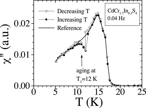
Figure 7. Reproduced from Figure 1 of Ref. [45]. Out-of-phase susceptibility χ′′ of the CdCr_1.7In_0.3S₄ spin glass. The solid line is measured upon heating the sample at a constant rate on 0.1 K/min (reference curve). Open diamonds: the measurement is done during cooling at this same rate, except that the cooling procedure has been stopped at 12 K during 7 h to allow for aging. Cooling then resumes down to 5 K: χ′′ is not influenced and goes back to the reference curve (chaos). This is termed rejuvenation. Solid circles: after this cooling procedure, the data is taken while reheating at the previous constant rate, exhibiting memory of the aging stage at 12 K.

This assignment has yet to be proven unequivocally. A very recent paper [18] by Paga et al. displayed the results of temperature cycling to explore this claim, and indeed to relate rejuvenation to the spin glass coherence length. Figure 8 reproduces their Figure 2. While Figure 8 appears definitive, there needs to be an exploration of $t_w^{\text{eff}}$ for temperature above and below the temperature for the onset of temperature chaos to arrive at an unequivocal relationship between rejuvenation and temperature chaos. For the moment, Figure 8 seems entirely consistent with that interpretation.

Figure 8

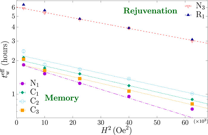
Figure 8. Reproduced from Figure 2 of Ref. [18]. We use the abbreviations N (native), R (rejuvenation), and C (cycle). By native, we mean the temperature is lowered from above T_g (here, T_g = 41.6 K to the lower temperature T₂ in the usual cycling protocol (here, T₂ = 26 K, t_w2 = 3 h), and the effective waiting time is given by the peak in S(t) for different magnetic fields H. The points are labeled N₃ in Figure 8. Next, the system is cooled from above T_g to the temperature T₁ = 30 K and aged for 1 h. The temperature is then dropped to T₂ = 26 K, and aged for 3 h. The points are labelled R₁ in Figure 8. As can be seen from the figure, the two procedures yield nearly exactly the same $t_w^{\text{eff}}$ for all values of H², independent of the aging at T₁. This is a clear demonstration of rejuvenation. In addition, the spin glass coherence lengths can be extracted from the slope of $t_w^{eff}vs{H}^2$. One finds ${\xi }_{N_3}/a_0=11.96(9)$ and ${\xi }_{R_1}/a_0=11.787(8)$, showing the development of spin glass order is the same without and with aging at T₁. Memory is measured through a full temperature cycle, from T₁, t_w1 → T₂, t_w2 → T₁ when $t_w^{\mathrm{e}\mathrm{ff}}$ is measured as rapidly as possible. The text discusses the physical meaning for the three protocols, C₁, C₂, and C₃.

2.5 Memory

Though rejuvenation in spin glasses is remarkable, the even more remarkable is memory. Once the system has rejuvenated back to the reference curve, upon reheating it traces out the same behavior as it exhibited upon cooling, even with temperature chaos between T₁ and T₂. This is explicitly demonstrated in Figure 7. On the surface it seems quite inconsistent. How can the system exhibit memory when it has experienced temperature chaos? There have been a multitude of papers and models that addressed this conundrum. Most involve heuristic models with adjustable parameters that can fit the data represented in Figure 7. A recent treatment [18] gives an interpretation that is free of real space models and the concomitant adjustable parameters, and is based upon the behavior of the spin glass coherence length. The beauty of this formulation is that every term in its interpretation can be tested experimentally, something that previous models lack.

The concept is as follows. Upon cooling the spin glass from above T_g to the first measuring temperature T₁, the system is aged for a time t_w1. As a consequence, the spin glass coherence length grow from nucleation to ξ(t_w1, T). When the temperature is then lowered to T₂, the correlations created at T₁ are essentially frozen. This concept has been introduced by Bouchaud et al. [45]. What is new is that, when the system is aged at T₂ for a time t_w2, the system has created new coherent regions that have nothing to do with those created at T₁. Hence, when heating back to T₂, the two correlated regions interfere, thereby reducing the spin glass coherence length from the native value created at T₁, t_w1.

This is exhibited explicitly in Figure 8 in the lower part of the figure. The C_n represent three separate temperature and waiting time cycles, and illustrate unequivocally the relationship between memory and competing coherence lengths. Each of the cycles has three steps: 1) the system is “prepared” at T₁ = 30 K by waiting for the same time t_w1 = 1 h 2) The temperature is then dropped to T₂ and the system is aged for t_w2. 3) The system is than heated back to T₁ = 30 K and $t_w^{\text{eff}}$ measured as rapidly as possible. C₁ sets T₂ = 26 K and t_w2 = 1/6 h. C₂ sets T₂ = 26 K and t_w2 = 3 h. Finally, C₃ sets T₂ = 16 K and t_w2 = 3 h. Memory is quantified by comparing the magnitude of the coherence length measured at step (3) with the native coherence length [the coherence length of the initially prepared state at step (1)]. If the two lengths are the same, memory is perfect. If after step (3), the measured coherence length is smaller than the initially prepared state at step (1), memory is less, a direct result of the interference of the two states. The slopes in Figure 8 are steeper, the larger the coherence length being measured because the volume of the correlated region is larger [Eq. 1].

Consider C₁. The system has “morphed” from the prepared state into a chaotic regime, but only aged for a short time (1/6 h). The coherence length in the chaotic state has grown during this time, so that its interference with the initially prepared coherence length is significant. Hence, the memory is less, exhibited by the shallower slope as compared to the native slope exhibited in Figure 8. Now, C₂ increases t_w2 to 3 h, so that the coherence length in the chaotic state can grow beyond it is value in C₁. This should lead to greater interference, a smaller memory, and a more shallow slope than found for C₁. This is explicit in Figure 8.

Finally, the C₃ protocol has the same t_w2 as C₂, but the temperature drop to T₂ is much greater, T₂ = 16 K. At such a low temperature, the growth of the chaotic coherence length is very slow (almost none), so there should be almost no interference, and the memory should be nearly perfect. This again is explicitly exhibited in Figure 8 where the slope of C₃ is close to the slope for the native slope.

These three temperature cycles, and their properties exhibited in Figure 8, are strong evidence for the interpretation of memory through interfering coherence volumes. This is at odds with Ref. [46] where it is argued that the coherence length returned to the native value upon reheating. By adjusting t_w2 one can change the value of ξ(T₁, t_w1, T₂, t_w2) at will, from no loss to complete loss of memory. This have been born out in our Figure 8, and also in independent experiments by Freedberg et al. [47].

3 Summary

The purpose of this paper is to display spin glass dynamics through the lens of the spin glass coherence length. We have shown how it use can unite the seeming independent features observed both in the laboratory and through simulations. They provide a unifying picture for what seem to be independent complex phenomena.

Data availability statement

The raw data supporting the conclusions of this article will be made available by the authors, without undue reservation.

Author contributions

JH: Visualization, Writing–original draft, Writing–review and editing. RO: Conceptualization, Data curation, Formal Analysis, Funding acquisition, Investigation, Project administration, Resources, Supervision, Validation, Visualization, Writing–original draft, Writing–review and editing.

Funding

The author(s) declare that financial support was received for the research, authorship, and/or publication of this article. This work has been supported by the U.S. Department of Energy, Office of Basic Energy Sciences, Division of Materials Science and Engineering, under Award DE-SC0013599.

Acknowledgments

We thank Dr. I. Paga for a close reading of this manuscript, and for her important insights.

Conflict of interest

The authors declare that the research was conducted in the absence of any commercial or financial relationships that could be construed as a potential conflict of interest.

The handling editor FRT declared a past co-authorship with the author RO.

Publisher’s note

All claims expressed in this article are solely those of the authors and do not necessarily represent those of their affiliated organizations, or those of the publisher, the editors and the reviewers. Any product that may be evaluated in this article, or claim that may be made by its manufacturer, is not guaranteed or endorsed by the publisher.

References

1. Joh YG, Orbach R, Wood GG, Hammann J, Vincent E. Extraction of the spin glass correlation length. Phys Rev Lett (1999) 82:438–41. doi:10.1103/PhysRevLett.82.438

CrossRef Full Text | Google Scholar

2. Marinari E, Parisi G, Ruiz-Lorenzo J, Ritort F. Numerical evidence for spontaneously broken replica symmetry in 3d spin glasses. Phys Rev Lett (1996) 76:843–6. doi:10.1103/PhysRevLett.76.843

PubMed Abstract | CrossRef Full Text | Google Scholar

3. Baity-Jesi M, Calore E, Cruz A, Fernandez LA, Gil-Narvion JM, Gordillo-Guerrero A, et al. Matching microscopic and macroscopic responses in glasses. Phys Rev Lett (2017) 118:157202. doi:10.1103/PhysRevLett.118.157202

PubMed Abstract | CrossRef Full Text | Google Scholar

4. Sherrington D, Kirkpatrick S. Solvable model of a spin-glass. Phys Rev Lett (1975) 35:1792–6. doi:10.1103/PhysRevLett.35.1792

CrossRef Full Text | Google Scholar

5. Mézard M, Parisi G, Sourlas N, Toulouse G, Virasoro M. Replica symmetry breaking and the nature of the spin glass phase. J Phys France (1984) 45:843–54. doi:10.1051/jphys:01984004505084300

CrossRef Full Text | Google Scholar

6. Parisi G. Spin glasses and fragile glasses: statics, dynamics, and complexity. Proc Natl Acad Sci (2006) 103:7948–55. doi:10.1073/pnas.0601120103

PubMed Abstract | CrossRef Full Text | Google Scholar

7. Parisi G. Toward a mean field theory for spin glasses. Phys Lett A (1979) 73:203–5. doi:10.1016/0375-9601(79)90708-4

CrossRef Full Text | Google Scholar

8. Parisi G. A sequence of approximated solutions to the s-k model for spin glasses. J Phys A: Math Gen (1980) 13:L115–21. doi:10.1088/0305-4470/13/4/009

CrossRef Full Text | Google Scholar

9. Hammann J, Lederman M, Ocio M, Orbach R, Vincent E. Spin-glass dynamics Relation between theory and experiment: a beginning. Physica A Stat Mech its Appl (1992) 185:278–94. doi:10.1016/0378-4371(92)90467-5

CrossRef Full Text | Google Scholar

10. Nordblad P, Svedlindh P, Lundgren L, Sandlund L. Time decay of the remanent magnetization in a cumn spin glass. Phys Rev B (1986) 33:645–8. doi:10.1103/PhysRevB.33.645

CrossRef Full Text | Google Scholar

11. Baity-Jesi M, Baños R, Cruz A, Fernandez L, Gil-Narvion J, Gordillo-Guerrero A, et al. Janus ii: a new generation application-driven computer for spin-system simulations. Comput Phys Commun (2014) 185:550–9. doi:10.1016/j.cpc.2013.10.019

CrossRef Full Text | Google Scholar

12. Baity-Jesi M, Calore E, Cruz A, Fernandez LA, Gil-Narvion JM, Gonzalez-Adalid Pemartin I, et al. Memory and rejuvenation effects in spin glasses are governed by more than one length scale. Nat Phys (2023) 19:978–85. doi:10.1038/s41567-023-02014-6

CrossRef Full Text | Google Scholar

13. de Almeida JRL, Thouless DJ. Stability of the sherrington-kirkpatrick solution of a spin glass model. J Phys A: Math Gen (1978) 11:983–90. doi:10.1088/0305-4470/11/5/028

CrossRef Full Text | Google Scholar

14. De Dominicis C, Giardina I. Random fields and spin glasses: a field theory approach. Cambridge University Press (2006). doi:10.1017/CBO9780511534836

CrossRef Full Text | Google Scholar

15. Belletti F, Cotallo M, Cruz A, Fernandez LA, Gordillo-Guerrero A, Guidetti M, et al. Nonequilibrium spin-glass dynamics from picoseconds to a tenth of a second. Phys Rev Lett (2008) 101:157201. doi:10.1103/PhysRevLett.101.157201

PubMed Abstract | CrossRef Full Text | Google Scholar

16. Belletti F, Cruz A, Fernandez LA, Gordillo-Guerrero A, Guidetti M, Maiorano A, et al. An in-depth view of the microscopic dynamics of ising spin glasses at fixed temperature. J Stat Phys (2009) 135:1121–58. doi:10.1007/s10955-009-9727-z

CrossRef Full Text | Google Scholar

17. Paga I, Zhai Q, Baity-Jesi M, Calore E, Cruz A, Fernandez LA, et al. Spin-glass dynamics in the presence of a magnetic field: exploration of microscopic properties. J Stat Mech Theor Exp (2021) 2021:033301. doi:10.1088/1742-5468/abdfca

CrossRef Full Text | Google Scholar

18. Collaboration J, Paga I, He J, Baity-Jesi M, Calore E, Cruz A, et al. arxiv: quantifying memory in spin glasses (2023).

Google Scholar

19. Paga I, Zhai Q, Baity-Jesi M, Calore E, Cruz A, Cummings C, et al. Superposition principle and nonlinear response in spin glasses. Phys Rev B (2023) 107:214436. doi:10.1103/PhysRevB.107.214436

CrossRef Full Text | Google Scholar

20. Koper GJM, Hilhorst HJ. A domain theory for linear and nonlinear aging effects in spin glasses. J Phys France (1988) 49:429–43. doi:10.1051/jphys:01988004903042900

CrossRef Full Text | Google Scholar

21. Fisher DS, Huse DA. Nonequilibrium dynamics of spin glasses. Phys Rev B (1988) 38:373–85. doi:10.1103/PhysRevB.38.373

PubMed Abstract | CrossRef Full Text | Google Scholar

22. Baity-Jesi M, Calore E, Cruz A, Fernandez LA, Gil-Narvion JM, Gordillo-Guerrero A, et al. Aging rate of spin glasses from simulations matches experiments. Phys Rev Lett (2018) 120:267203. doi:10.1103/PhysRevLett.120.267203

PubMed Abstract | CrossRef Full Text | Google Scholar

23. Zinn-Justin J. Quantum field theory and critical phenomena. In: International series of monographs on physics. Oxford University Press (2021). General theoretical arguments suggest that z_c is is also ξ independent at exactly T = T_g.

Google Scholar

24. Zhai Q, Harrison DC, Tennant D, Dahlberg ED, Kenning GG, Orbach RL. Glassy dynamics in cumn thin-film multilayers. Phys Rev B (2017) 95:054304. doi:10.1103/PhysRevB.95.054304

CrossRef Full Text | Google Scholar

25. Kenning GG, Tennant DM, Rost CM, da Silva FG, Walters BJ, Zhai Q, et al. End of aging as a probe of finite-size effects near the spin-glass transition temperature. Phys Rev B (2018) 98:104436. doi:10.1103/PhysRevB.98.104436

CrossRef Full Text | Google Scholar

26. Zhai Q, Martin-Mayor V, Schlagel DL, Kenning GG, Orbach RL. Slowing down of spin glass correlation length growth: simulations meet experiments. Phys Rev B (2019) 100:094202. doi:10.1103/PhysRevB.100.094202

CrossRef Full Text | Google Scholar

27. Malozemoff AP, Barbara B, Imry Y. Further studies of nonlinear susceptibility of GdAl and MnCu spin glasses. J Appl Phys (1982) 53:2205–7. doi:10.1063/1.330818

CrossRef Full Text | Google Scholar

28. Malozemoff AP, Imry Y, Barbara B. Scaling of susceptibility and the size of the critical region in an amorphous GdAl spin glass (invited). J Appl Phys (1982) 53:7672–7. doi:10.1063/1.330179

CrossRef Full Text | Google Scholar

29. Chandra P, Coleman P, Ritchey I. The anisotropic kagome antiferromagnet: a topological spin glass? J Phys France (1993) 3:591–610. doi:10.1051/jp1:1993104

CrossRef Full Text | Google Scholar

30. Lévy LP, Ogielski AT. Nonlinear dynamic susceptibilities at the spin-glass transition of ag:mn. Phys Rev Lett (1986) 57:3288–91. doi:10.1103/PhysRevLett.57.3288

PubMed Abstract | CrossRef Full Text | Google Scholar

31. Lévy LP. Critical dynamics of metallic spin glasses. Phys Rev B (1988) 38:4963–73. doi:10.1103/PhysRevB.38.4963

CrossRef Full Text | Google Scholar

32. Baity-Jesi M, Baños RA, Cruz A, Fernandez LA, Gil-Narvion JM, Gordillo-Guerrero A, et al. Critical parameters of the three-dimensional ising spin glass. Phys Rev B (2013) 88:224416. doi:10.1103/PhysRevB.88.224416

CrossRef Full Text | Google Scholar

33. Bert F, Dupuis V, Vincent E, Hammann J, Bouchaud JP. Spin anisotropy and slow dynamics in spin glasses. Phys Rev Lett (2004) 92:167203. doi:10.1103/PhysRevLett.92.167203

PubMed Abstract | CrossRef Full Text | Google Scholar

34. Fernandez LA, Marinari E, Martin-Mayor V, Parisi G, Yllanes D. Temperature chaos is a non-local effect. J Stat Mech Theor Exp (2016) 2016:123301. doi:10.1088/1742-5468/2016/12/123301

CrossRef Full Text | Google Scholar

35. Sasaki M, Nemoto K. Memory effect, rejuvenation and chaos effect in the multi-layer random energy model. J Phys Soc Jpn (2000) 69:2283–90. doi:10.1143/JPSJ.69.2283

CrossRef Full Text | Google Scholar

36. Sasaki M, Martin OC. Discreteness and entropic fluctuations in generalized-random-energy-model-like systems. Phys Rev B (2002) 66:174411. doi:10.1103/PhysRevB.66.174411

CrossRef Full Text | Google Scholar

37. Sales M, Bouchaud JP, Ritort F. Temperature shifts in the sinai model: static and dynamical effects. J Phys A: Math Gen (2003) 36:665–84. doi:10.1088/0305-4470/36/3/306

CrossRef Full Text | Google Scholar

38. Rizzo T. Ultrametricity between states at different temperatures in spin-glasses. Eur Phys J B (2002) 29:425–35. doi:10.1140/epjb/e2002-00274-x

CrossRef Full Text | Google Scholar

39. Zhai Q, Orbach RL, Schlagel DL. Evidence for temperature chaos in spin glasses. Phys Rev B (2022) 105:014434. doi:10.1103/PhysRevB.105.014434

CrossRef Full Text | Google Scholar

40. Baity-Jesi M, Calore E, Cruz A, Fernandez LA, Gil-Narvion J, Gonzalez-Adalid Pemartin I, et al. Temperature chaos is present in off-equilibrium spin-glass dynamics. Commun Phys (2021) 4:74. doi:10.1038/s42005-021-00565-9

CrossRef Full Text | Google Scholar

41. Bray AJ, Moore MA. Chaotic nature of the spin-glass phase. Phys Rev Lett (1987) 58:57–60. doi:10.1103/PhysRevLett.58.57

PubMed Abstract | CrossRef Full Text | Google Scholar

42. Jönsson PE, Yoshino H, Nordblad P. Symmetrical temperature-chaos effect with positive and negative temperature shifts in a spin glass. Phys Rev Lett (2002) 89:097201. doi:10.1103/PhysRevLett.89.097201

PubMed Abstract | CrossRef Full Text | Google Scholar

43. Kondor I. On chaos in spin glasses. J Phys A: Math Gen (1989) 22:L163–8. doi:10.1088/0305-4470/22/5/005

CrossRef Full Text | Google Scholar

44. Billoire A, Coluzzi B. Magnetic field chaos in the sherrington-kirkpatrick model. Phys Rev E (2003) 67:036108. doi:10.1103/PhysRevE.67.036108

PubMed Abstract | CrossRef Full Text | Google Scholar

45. Jonason K, Vincent E, Hammann J, Bouchaud JP, Nordblad P. Memory and chaos effects in spin glasses. Phys Rev Lett (1998) 81:3243–6. doi:10.1103/PhysRevLett.81.3243

CrossRef Full Text | Google Scholar

46. Bouchaud JP, Dupuis V, Hammann J, Vincent E. Separation of time and length scales in spin glasses: temperature as a microscope. Phys Rev B (2001) 65:024439. doi:10.1103/PhysRevB.65.024439

CrossRef Full Text | Google Scholar

47. Freedberg J, Meese WJ, He J, Schlagel DL, Dahlberg ED, Orbach RL. arxiv: on the nature of memory and rejuvenation in glassy systems (2023).

Google Scholar