A lidar for detecting atmospheric turbulence based on modified Von Karman turbulence power spectrum

1 Introduction

Atmospheric turbulence is universal in the atmosphere, and its state is always flowing and has no rules. It is mainly concentrated in the boundary layer at the bottom of the atmosphere. It can be used to transfer the energy between the atmosphere and the surface, and carry out the transformation and exchange of materials. The formation of turbulence is due to the temperature changes in the atmosphere and the random change of radiant heat convection on the surface, resulting in random fluctuations in the atmospheric refractive index at different locations in the atmosphere, which will lead to the distortion of the laser wave front and destroy the coherence of the laser, which will seriously affect the optical transmission quality of the laser, and optical turbulence effect will occur when transmitted in turbulence. The degradation of coherence will seriously weaken the optical quality of laser, causing random drift of light, redistribution of laser energy on the beam cross-section, fluctuation of light wave arrival angle, and fluctuation of light intensity on a certain receiving area [1]. The random drift of the laser beam brings difficulties to the reception of optical communication, and the fluctuation of light intensity on the receiving area introduces noise into the communication signal. Physical quantities often used to measure atmospheric turbulence information: atmospheric refractive index structure constant $C_n^2$ and atmospheric coherence length $r_0$ (also known as Fried constant), which represents the spatial coherence characteristics of light waves on cross sections when the beam is transmitted in atmospheric turbulence [2]. The distribution of atmospheric turbulence intensity with the measured height is called atmospheric turbulence profile. Therefore, local climate change and precipitation can be understood by obtaining real-time and accurate atmospheric turbulence profile.

Establishing an analytical model for turbulence effects can quickly estimate the degradation of laser coherence caused by turbulence. This study is based on the modified Von Karman turbulence, which takes into account the size of the inner and outer scales of turbulence, so the research results are more consistent with the actual situation. As early as 1976, people began to use the “multi phase screen method” to simulate the impact of turbulent atmosphere on laser transmission, and since then this method has been widely used in the study of the transmission of light waves in atmospheric turbulence [3]. There are many methods that have been developed to generate random phase screens that conform to the characteristics of turbulent atmosphere, mainly including the “power spectrum inversion method” and the “Zernike polynomial expansion method”. The power spectrum method has been widely used in the generation of turbulent phase screens. In recent years, an increasing number of research reports have shown that turbulence in the top troposphere and stratosphere of the atmosphere has deviated from the Kolmogorov turbulence statistical law, that is, Kolmogorov turbulence is not the only turbulence model present in the atmosphere.

In recent years, extensive research has been conducted on modified Von Karman turbulence. In 2012, Wu et al. conducted a study on the intensity scintillation of coherent synthesized array beams propagating in turbulent atmospheres [4]. In 2012, Cui et al. developed an light intensity scintillation lidar for atmospheric turbulence detection, and obtained the scintillation index and atmospheric refractive index structure constant in the horizontal direction through experiments [5]. In 2015, based on the modified Rytov method, Ke et al. used the partially coherent Gaussian Schell (GSM) beam model and combined it with Andrews’ phenomenological scintillation model to derive the variance expression of logarithmic light intensity fluctuations for different turbulence scenarios [6].

In 2015, Wei et al. studied the scintillation index of echoes in tilted atmospheric turbulence, and the expression for obtaining the axial scintillation index of the echo [7]. In 2015, Chen et al. conducted an experimental study on the propagation characteristics of vortex beams in atmospheric turbulence and the scintillation index of vortex beams with different topological charges. The results show that in weak turbulence state, the scintillation index of vortex beam is higher than that of Gaussian beam, but in strong turbulence state, after propagating for 400 m, the scintillation index of vortex beam is lower than that of Gaussian beam [8]. In 2016, Zhu Ling et al. from Beijing University of Posts and Telecommunications used the modified Von Karman theory as a model, compared the closeness of phase screens generated by different algorithms to actual turbulence [9]. In 2017, Wang et al. studied the intensity distribution and fluctuation characteristics of Gaussian laser under different weather conditions, and analyzed the atmospheric scintillation index [10].

In 2020, Aly et al. derived the oblique path scintillation index of spherical waves in a closed form and proposed a polynomial model for refractive index structural parameters [11]. In 2018, Wang et al. have developed a rigorous physical and mathematical beam model that effectively suppresses the scintillation of atmospheric turbulent light intensity [12]. In 2021, Mert et al. studied the propagation changes of hyperbolic sine Gaussian beams and their point like scintillation in turbulent atmosphere. Under scintillation conditions, the scintillation index of all selected HSG beams was lower than that of Gaussian beams [13]. In 2022, Wu et al. established a mathematical model for the variance of logarithmic light intensity fluctuations under near-ground oblique atmospheric turbulence and multi beam propagation in free space optical communication based on the theory of multi beam propagation, and obtained the light intensity fluctuation characteristics of single beam and multi beam [14].

In this paper, based on the modified Von Karman turbulence refractive index power spectrum, the power spectrum method and the Zernike polynomial method are used for low-frequency compensation to simulate the modified Von Karman turbulence phase screen. The influence of phase screen parameters on the simulation results of the modified Von Karman turbulence is discussed. In order to verify the feasibility of Mie-Scattering lidar for detecting atmospheric turbulence based on modified Von Karman turbulence power spectrum model, some simulations were conducted on the beam drift, angle of arrival fluctuations, and intensity scintillation of Gaussian beams, which further determine the reliability of Mie-scattering lidar for detecting modified Von Karman turbulence. Based on the guidance for simulation analysis, a Mie-scattering lidar system for detecting the intensity of atmospheric turbulence is developed, and the atmospheric turbulence profile is obtained by inversion of detected scintillation index.

2 The generation of principle and implementation of turbulent phase screen

2.1 Phase screen simulation theory

For the research of atmosphere turbulence, Kolmogorov theory is currently the most widely used theory [15], which is the foundation of other turbulence theories and defines some important parameters to describe the physical characteristics of turbulence. Firstly, the inner scale is $l_0$ and the outer scale is $L_0$, and L₀>>l₀. Secondly, the atmospheric refractive index structure constant $C_n^2$, the turbulence intensity is proportional to $C_n^2$; Thirdly, the atmospheric coherence length $r_0$, and turbulence intensity is inversely proportional to $r_0$. The relation between atmospheric refractive index structure constant $C_n^2$ and atmospheric coherence length is given in Eq. 1 [9]:

$r_0={\left[0.423k^2\sec \left(\zeta \right){\displaystyle \underset{path}{\int }}{C}_n^2\left(z\right)dz\right]}^{-3/5}(1)$

This describes the integral of $C_n^2$ over the transmission path, where $k=2\pi /\lambda$, it is the laser wave number, $\zeta$ is the zenith Angle of the beam transmission.

The propagation of light waves in random media can be divided into two processes [16]: the propagation process of light waves in vacuum and the wave front phase modulation process related to the fluctuation of refractive index of the medium, as shown in Figure 1.

Figure 1

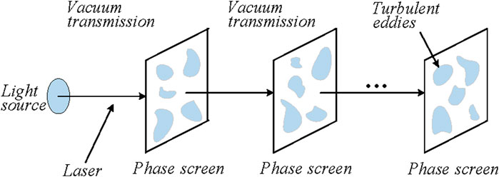
Figure 1. Simulation of light transmission under atmospheric turbulence conditions.

Through the decomposition process, we can segment the turbulent path into a set of thin planes parallel to each other and perpendicular to the direction of propagation. The light field travels from the front surface of each thin plane to the back surface through a plane of thickness $\Delta z$, on which phase modulation is performed. The light field then travels through the vacuum and continues to travel in the same way.

At present, the simulation methods for turbulent random phase screens are basically divided into two categories: one is the power spectrum inversion method, which has the characteristics of rich high-frequency components and insufficient low-frequency components; Another is Zernike polynomial method, which has the characteristics of rich low-frequency components and insufficient high-frequency components. The power spectrum inversion method is more universal; however, the Zernike polynomial method is only applicable to Kolmogorov spectra. In this paper, considering the characteristics of traditional spectral inversion methods and Zernike polynomial methods, the Zernike polynomial method is used to compensate for low frequency in the power spectral inversion method and improve the accuracy of the phase screen.

2.2 FFT method phase screen

FFT spectrum inversion method is also power spectrum inversion method, obtains the phase distribution of atmospheric disturbances based on the power spectral density function of atmospheric turbulence.

The power spectrum expression under the modified Von Karman model is given in Eq. 2 [2]:

${\varphi }_n\left(\kappa \right)=0.033C_n^2\frac{\exp \left(-\frac{{\kappa }^2}{{{\kappa }_m}^2}\right)}{{\left({\kappa }^2+{{\kappa }_0}^2\right)}^{11/6}},0\le \kappa \le \infty (2)$

where ${\kappa }_0=2\pi /L_0$, ${\kappa }_m=5.92/l_0$. Using the modified Von Karman turbulence spectrum model, and performing fast Fourier transform, the following form can be obtained (Eq. 3) [17]:

$\begin{array}{l}\phi \left(m\Delta x,n\Delta y\right)=\frac{2\pi k}{N}{\left(\frac{0.033C_n^2\Delta z2\pi }{\Delta x\Delta y}\right)}^{1/2}{\displaystyle \sum _{m^{\prime }=1}^N}{\displaystyle \sum _{n^{\prime }=1}^N}\left\{R\left(m^{\prime },n^{\prime }\right)\right.\\ \times \exp \left(\frac{j2\pi m{m}^{\prime }}{N}+\frac{j2\pi n{n}^{\prime }}{N}\right)\times {\left.\frac{\exp \left(-A/{{\kappa }_m}^2\right)}{{\left(A+{{\kappa }_0}^2\right)}^{11/6}}\right\}}^{1/2}\end{array}(3)$

where $A={\left[2\pi m^{\prime }/\left(N\Delta x\right)\right]}^2+{\left[2\pi n^{\prime }/\left(N\Delta y\right)\right]}^2$.

2.3 Zernike polynomial method phase screen

The Zernike polynomial is composed of an infinite sum of items, each of which is obtained by multiplying the coefficients of the previous term and the formula, and the sum of the products is the final result. Polynomials form a complete set of standard orthogonal bases, each corresponding to a unique type of phase distortion, such as defocus, spherical aberration, etc. The atmospheric turbulence distortion wavefront $\varphi \left(r\right)$ can be decomposed into orthogonal Zernike polynomials in the circular domain using Eq. 4 [18]:

$\varphi \left(r\right)={\displaystyle \sum _{j=1}^{\infty }}{a}_j\cdot Z_j\left(r\right)(4)$

where, j is the order, $a_j$ is the coefficient of the Zernike polynomial of order j, $Z_j\left(r\right)$ is the jth-order Zernike polynomial.

Using a linear combination of several Zernike polynomials to represent the atmospheric turbulence phase screen, the expression can be written as in Eq. 5 [17]:

${\phi }_{LF}\left(x,y\right)={\displaystyle \sum _{j=1}^{\infty }}{a}_j\cdot Z_j\left(x,y\right)(5)$

Among them, the mean of the coefficients of various Zernike polynomials is 0. Through using the covariance matrix of Zernike polynomial coefficients, and performing matrix singular value decomposition to obtain the Zernike polynomial coefficients of the wavefront phase, a phase screen can been generated finally.

There is a statistical correlation between various Zernike patterns, the covariance matrix ${\mathrm{\Gamma }}_a$ of the Zernike coefficient vector $a$ of the atmospheric wavefront gives the covariance expression between the items $i$ and $j$ Zernike polynomial coefficients as in Eq. 6 [18]:

When $\left(i-j\right)=even$,

$〈a_i{a}_j〉={\left(\frac{D}{r_0}\right)}^{5/3}\frac{2.246{\left(-1\right)}^{\left(n_i+n_j-2m_i\right)/2}\sqrt{\left(n_i+1\right)\left(n_j+1\right)}\mathrm{\Gamma }\left(\frac{14}{3}\right)\mathrm{\Gamma }\left(\left(n_i+n_j-\frac{5}{3}\right)/2\right)}{\mathrm{\Gamma }\left(\left(n_i-n_j+\frac{17}{3}\right)/2\right)\mathrm{\Gamma }\left(\left(n_j-n_i+\frac{17}{3}\right)/2\right)\mathrm{\Gamma }\left(\left(n_i+n_j+\frac{23}{3}\right)/2\right)}{\delta }_{m_i{m}_j}(6)$

When $\left(i-j\right)=odd$, $〈a_i{a}_j〉=0$.

Where $〈〉$ represents the ensemble average of signals, D is the aperture of the optical system, $r_0$ is the atmospheric coherence length, $\mathrm{\Gamma }$ is a gamma function, $n_i$ and $m_i$ is the radial and angular levels corresponding to $Z_i$, $n_j$ and $m_j$ is the radial and angular levels corresponding to $Z_j$.Then the singular value decomposition is carried out.

From the above equations, we can simulate the phase screens of atmospheric turbulence at different intensities. The high frequency component of the Zernike phase screen is severely missing, while the low frequency component is abundant. Increasing the order of Zernike polynomials can compensate for the insufficient high-frequency of the phase screen generated by Zernike polynomial method. Therefore, the low-frequency compensation power spectrum inversion method is based on the power spectrum inversion method and uses the Zernike polynomial method to compensate for the missing low-frequency components in the power spectrum inversion method. The numerical simulation phase screen is generated by the superposition of low-frequency and high-frequency components, where the high-frequency components are generated by the traditional spectrum inversion method, and the low-frequency components are obtained by the Zernike polynomial method. The turbulent phase screen after low-frequency compensation is obtained as in Eq. 7:

$\begin{array}{l}\phi \left(x,y\right)=C{\displaystyle \sum _{{\kappa }_x}}{\displaystyle \sum _{{\kappa }_y}}a\left({\kappa }_x,{\kappa }_y\right)\sqrt{{\varphi }_n\left({\kappa }_x,{\kappa }_y\right)}\\ \exp \left(i\left({\kappa }_{x}x+{\kappa }_{y}y\right)\right)+{\displaystyle \sum _{j=1}^{\infty }}{a}_j\cdot Z_j\left(x,y\right)\end{array}(7)$

2.4 Evaluation of phase structure function

With the continuous progress of theoretical research, it has been discovered that there are disadvantages in the Kolmogorov model. The inner and outer scales in actual turbulent environments cannot be as perfect as approximate conditions, nor can they guarantee an always isotropic and uniform environment. In order to better match the actual turbulent environment, a modified Von Karman model has been developed based on the original model. It specifies the specific numerical values for inner and outer scales, and introduces a Bessel function in the structural function, which can better simulate the actual situation of turbulence.

The statistical characteristics of atmospheric turbulence phase can be described using the phase structure function. The structural function form under the modified Von Karman model is defined as in Eq. 8 [6]:

$\begin{array}{l}{D}_{\varphi }^{theory}\left(r\right)=\frac{2\left(11/6\right)!}{2^{5/6}{\pi }^{8/3}}{\left[\frac{24}{5}\left(\frac{6}{5}\right)!\right]}^{5/6}{\left(r_0{f}_0\right)}^{-5/3}\\ \left[\frac{\left(5/6\right)!}{2^{1/6}}-{\left(2\pi r{f}_0\right)}^{5/6}{K}_{5/6}\left(2\pi r{f}_0\right)\right]\end{array}(8)$

where the abscissa r is the distance between any two points on the two-dimensional plane where the telescope enters the pupil; Ordinate $D_{\varphi }^{theory}\left(r\right)$ is the value of the phase structure function; $K_{5/6}\left(\cdot \right)$ is the second type of modified Bessel function. This form introduces complex calculations such as the second type of modified Bessel function and factorial. The inner and outer scales specify the size range of turbulent air masses, and the value of the structural function represents the disturbance energy that the air masses can possess.

2.5 Simulation results and validation of spectral inversion method

When using the power spectrum method to simulate the modified Von Karman turbulent phase screen. According to the relevant requirements of the simulation parameter range [19], the simulation parameters are set as: the wavelength of light wave is 0.532 μm, the atmospheric coherence length is r₀ = 1.5, 0.15, and 0.01 m, respectively, the square phase screen with length and width of 3 m, the number of grids is 1024 × 1024, the transmission distance is 1500 m, the phase screen spacing is Δz = 100 m, inner scale of turbulence is 0.01 m, outer scale of turbulence is 1 m, and the Zernike polynomial order is 8. The simulation results are shown in Figure 2, and the phase structure function is shown in Figure 3.

Figure 2

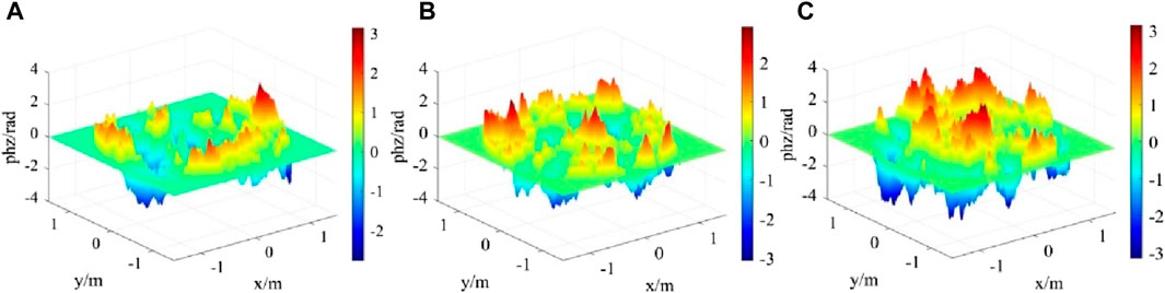
Figure 2. Uncompensated FFT phase screen under three turbulence intensities (A) r₀ = 2 m (B) r₀ = 0.15 m (C) r₀ = 0.01 m.

Figure 3

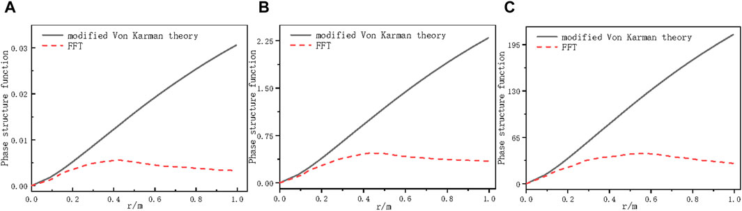
Figure 3. Phase structure function curves of uncompensated FFT under three turbulence intensities (A) r₀ = 2 m PSF curve (B) r₀ = 0.15 m PSF curve (C) r₀ = 0.01 m PSF curve.

From Figure 2, it can be seen that different turbulence intensities have a significant impact on the spectral width of the phase screen. The stronger the atmospheric turbulence intensity, the greater the phase fluctuation of the phase screen.

From Figure 3, it can be seen that as the turbulence intensity continues to increase, the value of the phase structure function also continues to increase, indicating that the energy in the vortex is constantly increasing and the disturbance effect is increasing; When the r value is small, the value of the phase structure function approaches the theoretical value, indicating that the high-frequency component of the phase screen is rich and the low-frequency component is insufficient.

2.6 Zernike polynomial low frequency compensation results and verification

The Zernike polynomial low-frequency compensation power spectrum method is used to simulate the modified Von Karman turbulent phase screen, the simulation parameters are set as: the wavelength of light wave is 0.532 μm, the atmospheric coherence length is r₀ = 1.5, 0.15, and 0.01 m, respectively, the square phase screen with length and width of 3 m, the number of grids is 1024 × 1024, the transmission distance is 1500 m, the phase screen spacing is Δz = 100 m, inner scale of turbulence is 0.01 m, outer scale of turbulence is 1 m, and the Zernike polynomial order is 8. The simulation results are shown in Figure 4.

Figure 4

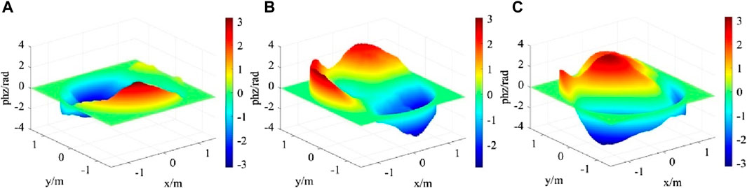
Figure 4. Zernike polynomial low-frequency compensation FFT phase screen under three turbulence intensities (A) r₀ = 2 m (B) r₀ = 0.15 m (C) r₀ = 0.01 m.

From Figure 4, the overall phase screen is relatively smooth. The smaller the atmospheric coherence length, the greater the phase fluctuation of the phase screen. In practical applications, relevant parameters should be selected based on the parameters of the laser emission system and the actual situation of the atmospheric environment.

When the simulation parameters are set as: the wavelength of light wave is 0.532 μm, the atmospheric coherence length is r₀ = 1.5 m, the square phase screen with length and width of 3 m, the number of grids is 1024 × 1024, the transmission distance is 1500 m, the phase screen spacing is Δz = 50, 100, and 150 m, respectively, inner scale of turbulence is 0.01 m, outer scale of turbulence is 1 m, and the Zernike polynomial order is 8. The simulation results are shown in Figure 5.

Figure 5

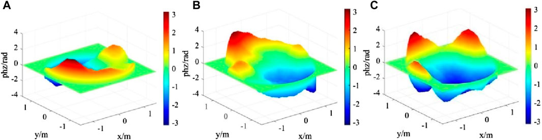
Figure 5. Zernike polynomial low-frequency compensated FFT phase screen under moderate turbulence with different phase screen spacing (A) Δz = 50 m (B) Δz = 100 m (C) Δz = 150 m.

From Figure 5, the different phase screen spacing has a significant impact on the amplitude width of the phase screen. The larger the phase screen spacing, the greater the phase fluctuation of the phase screen.

When the simulation parameters are: the wavelength of light wave is 0.532 μm, the atmospheric coherence length is r₀ = 0.15 m, the square phase screen with length and width of D = 1.5, 2.4, and 3 m, respectively, the number of grids is 1024 × 1024, the transmission distance is 1500 m, the phase screen spacing is Δz = 100 m, inner scale of turbulence is 0.01 m, outer scale of turbulence is 1m, and the Zernike polynomial order is 8. The simulation results are shown in Figure 6.

Figure 6

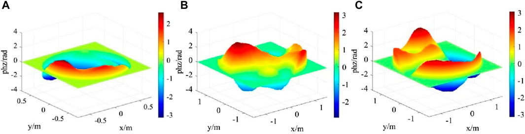
Figure 6. .Zernike polynomial low-frequency compensated FFT phase screen under moderate turbulence with different phase screen widths (A) D = 1.5 m (B) D = 2.4 m (C) D = 3 m.

From Figure 6, the different phase screen widths have a significant impact on the amplitude width of the phase screen, the larger the phase screen width, the greater the phase fluctuation of the phase screen.

When the simulation parameters are set as follows: the wavelength of light wave is 0.532 μm, the atmospheric coherence length is r₀ = 0.15 m, the square phase screen with length and width of D = 3 m, the number of grids is 1024 × 1024, the transmission distance is 1500 m, the phase screen spacing is Δz = 100 m, inner scale of turbulence is 0.01 m, outer scale of turbulence is 1 m, the Zernike polynomial order is eight and 38, respectively. The simulation results are shown in Figure 7.

Figure 7

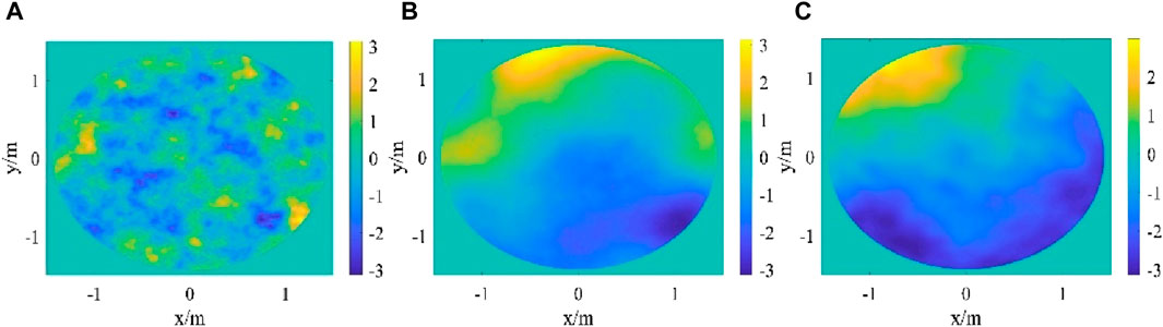
Figure 7. Zernike polynomial low-frequency compensated FFT phase screen with different orders of moderate turbulence (A) Uncompensated FFT (B) 8 order Zernike polynomial (C) 38 order Zernike polynomial.

From Figure 7, the phase screen has rich low-frequency components and very smooth phase fluctuations through eight-order Zernike polynomial compensation. After compensating with the 38th order Zernike polynomial, the low-frequency components of the phase screen are also very rich, but the phase fluctuations are no longer smooth. As mentioned above, the Zernike polynomial phase screens have the characteristics of rich low-frequency components and insufficient high-frequency components, as the order of Zernike polynomials increases, the high-frequency component of the phase screen increases, and the phase screen gradually becomes less smooth. Therefore, lower-order Zernike for low-frequency compensation has a better effect than higher-order Zernike for low-frequency compensation, and the phase screen is smoother. In this paper, an eight-order Zernike polynomial is selected to compensate for the missing low-frequency components in the power spectrum method and improve the accuracy of the phase screen.

To analyze the performance of the Zernike polynomial low-frequency compensation, a phase structure function was used for statistical analysis. The phase screen generated before and after the Zernike polynomial low frequency compensation is statistically analyzed, and its phase structure function is compared with the theoretical phase structure function of atmospheric turbulence. The comparison results are shown in Figure 8.

Figure 8

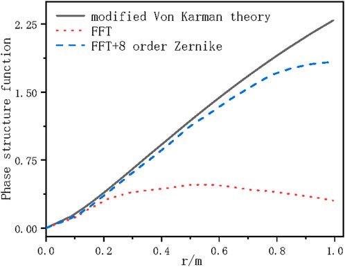
Figure 8. Zernike polynomial low-frequency compensated FFT Phase structure function.

It can be seen that the phase screen simulated using the power spectrum method before adding low-frequency compensation is relatively close to the theoretical value curve in the high-frequency region, but has a significant difference from the theoretical value in the low-frequency region. After eight-order Zernike polynomial low-frequency compensation, the phase structure function in the low-frequency region is closer to the theoretical value curve, which indicating that the compensation is effective.

3 Simulation of light intensity transmitted by gaussian beams in modified von karman turbulence

3.1 The intensity of the gaussian beams fluctuates

When considering the inner and outer scales, the axial scintillation index of the Gaussian beam is obtained asin Eqs 9–16 [20, 21]:

${\sigma }_I^2\left(r,z\right)=\exp \left[{\sigma }_{\ln x}^2\left(l_0\right)-{\sigma }_{\ln x}^2\left(L_0\right)+\frac{0.51{\sigma }_G^2}{{\left(1+0.69{\sigma }_G^{12/5}\right)}^{5/6}}\right]-1(9)$

where

$\begin{array}{l}{\sigma }_{\ln x}^2\left(l_0\right)=0.49{\sigma }_1^2\left(\frac{1}{3}-\frac{1}{2}\overline{\mathrm{\Theta }}+\frac{1}{5}{\overline{\mathrm{\Theta }}}^2\right){\left(\frac{{\eta }_x{Q}_l}{{\eta }_x+Q_l}\right)}^{7/6}\\ \times \left[1+1.75{\left(\frac{{\eta }_x}{{\eta }_x+Q_l}\right)}^{1/2}-0.25{\left(\frac{{\eta }_x}{{\eta }_x+Q_l}\right)}^{7/12}\right]\end{array}(10)$

$\begin{array}{l}{\sigma }_{\ln x}^2\left(L_0\right)=0.49{\sigma }_1^2\left(\frac{1}{3}-\frac{1}{2}\overline{\mathrm{\Theta }}+\frac{1}{5}{\overline{\mathrm{\Theta }}}^2\right){\left(\frac{{\eta }_{x0}{Q}_l}{{\eta }_{x0}+Q_l}\right)}^{7/6}\\ \times \left[1+1.75{\left(\frac{{\eta }_{x0}}{{\eta }_{x0}+Q_l}\right)}^{1/2}-0.25{\left(\frac{{\eta }_{x0}}{{\eta }_{x0}+Q_l}\right)}^{7/12}\right]\end{array}(11)$

$\begin{array}{l}{\sigma }_G^2=3.86{\sigma }_1^2\left\{0.4\frac{{\left[{\left(1+2\mathrm{\Theta }\right)}^2+{\left(2\mathrm{\Lambda }+3/Q_l\right)}^2\right]}^{11/12}}{{\left[{\left(1+2\mathrm{\Theta }\right)}^2+4{\mathrm{\Lambda }}^2\right]}^{1/2}}\left.\sin \left(\frac{11}{6}{\phi }_1+{\phi }_2\right)\right]\right.\\ -\frac{6\mathrm{\Lambda }}{Q_l^{11/6}\left[{\left(1+2\mathrm{\Theta }\right)}^2+4{\mathrm{\Lambda }}^2\right]}\left.-\frac{11}{6}{\left(\frac{1+0.31\mathrm{\Lambda }{Q}_l}{Q_l}\right)}^{5/6}\right\}\end{array}(12)$

where

$\begin{array}{l}\frac{1}{{\eta }_x}=\frac{0.38}{1-3.2\overline{\mathrm{\Theta }}+5.29{\overline{\mathrm{\Theta }}}^2}+0.47\\ \times {\sigma }_1^2{Q}_l^{1/6}{\left(\frac{1/3-0.5\overline{\mathrm{\Theta }}+0.2{\overline{\mathrm{\Theta }}}^2}{1+2.2\overline{\mathrm{\Theta }}}\right)}^{6/7}\end{array}(13)$

${\eta }_{x0}=\frac{{\eta }_x{Q}_0}{{\eta }_x+Q_0}(14)$

${\phi }_1={\tan }^{-1}\left[\frac{\left(1+2\mathrm{\Theta }\right)Q_l}{3+2\mathrm{\Lambda }{Q}_l}\right](15)$

${\phi }_2={\tan }^{-1}\left[\frac{2\mathrm{\Lambda }}{1+2\mathrm{\Theta }}\right](16)$

The parameter $Q_0=64{\pi }^{2}z/k{L}_0^2$ and $Q_l=10.89z/k{l}_0^2$ correspond to the relevant terms of the inner and outer scales, respectively.

Figure 9 shows the variation of Gaussian beam scintillation index with Rytov variance, taking into account the inner and outer scales of turbulence, based on the above equation, in which the wavelength of light wave is 0.532 μm, the waist radius is 20 cm, the inner scale is l₀ = 0.01 m, the outer scale is L₀ = 1 m, and the turbulence intensity is $C_n^2=4\times {10}^{-13}{m}^{-2/3}$. From Figure 10, the trend of the four curves is roughly the same, that is, as the Rytov variance continues to increase, the scintillation index rapidly increases to a peak, and then slowly decreases. In the weak fluctuation region, the difference in scintillation index values is not significant, while in the medium strong turbulence region, the difference in scintillation index is more significant: when the Rytov variance is the same, as the inner and outer scales of the turbulence increase, the scintillation index also increases.

Figure 9

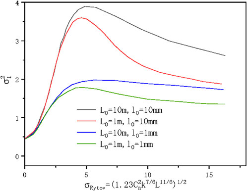
Figure 9. The scintillation index curve of Gaussian beam with different values of inner and outer scales.

Figure 10

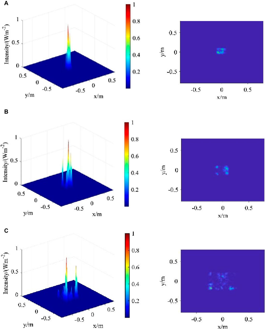
Figure 10. Light intensity distribution map under three turbulence intensities (A) r₀ = 2 m (B) r₀ = 0.15 m (C) r₀ = 0.01 m.

3.2 Simulation of the intensity scintillation effect of Gaussian beams propagating in modified Von Karman turbulence

Based on the fundamental mode Gaussian beam field intensity formula [14], the intensity distribution of Gaussian beams after propagation in atmospheric turbulence is simulated. Figure 11 shows the simulation results, in which the wavelength of light wave is 0.532 μm, the waist radius of a Gaussian beam is 20 cm, the square phase screen with length and width of D = 1.6 m, the number of grids is 1024 × 1024, the transmission distance is 1500 m, the phase screen spacing is Δz = 100 m, the order of Zernike polynomial is selected to be 8, and the atmospheric coherence length is r₀ = 2, 0.15, and 0.01 m, respectively.

Figure 11

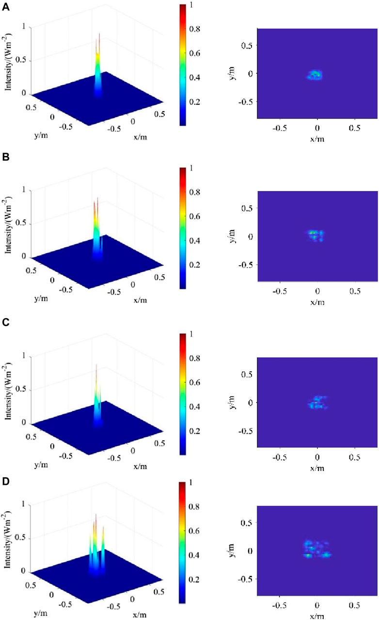
Figure 11. Light intensity distribution map under different conditions (A) L = 1500 m, Δz = 80 m (B) L = 1500 m, Δz = 200 m (C) L = 6500 m, Δz = 80 m (D) L = 6500 m, Δz = 200 m.

In Figure 10, when a Gaussian beam propagates in a turbulent atmosphere, the spot image of the Gaussian beam will disperse as the atmospheric coherence length decreases. That is, the stronger the turbulence intensity, the greater the degree of dispersion of the Gaussian beam’s spot. This indicates that the turbulence intensity has a significant impact on the overall intensity and uniformity of the light intensity.

Figure 11 shows the distribution of light intensity under moderate turbulence intensity, in which the wavelength of light wave is 0.532 μm, the waist radius of a Gaussian beam is 20 cm, the square phase screen with length and width of D = 1.6 m, the number of grids is 1024 × 1024, the transmission distance is L = 1500 and 6500 m, respectively, the phase screen spacing is Δz = 80 and 100 m, respectively, and the order of Zernike polynomial was selected to be 8.

It can be seen that when a Gaussian beam propagates in a turbulent atmosphere, the spot image of the Gaussian beam will disperse with the increase of transmission distance and phase screen spacing. That is, the greater the transmission distance, the greater the degree of dispersion of the Gaussian beam’s spot, which indicating that the transmission distance has a significant impact on the overall intensity and uniformity of light intensity.

The atmospheric turbulence fluctuation can be divided into two types: strong fluctuation and weak fluctuation. Based on a large amount of data and experimental detection, most turbulence situations are currently under weak fluctuation conditions. This paper mainly focuses on the corresponding research in weak fluctuation situations. In the state of weak turbulence fluctuations, Rytov exponent is defined as an important parameter to measure the fluctuation conditions, which is defined as in Eq. 17 [22]:

${\sigma }_{Rytov}^2\left(L\right)=1.23C_n^2{k}^{7/6}{L}^{11/6}(17)$

where, $C_n^2$ is the atmospheric refractive index structure constant, $k$ is the wave number, $L$ is the transmission distance. When ${\sigma }_{Rytov}^2<1$, the corresponding interval is the weak turbulence zone; When ${\sigma }_{Rytov}^2\sim 1$, the corresponding interval is the medium turbulence zone; when ${\sigma }_{Rytov}^2>1$, the corresponding interval is the strong turbulence zone. It is often not enough to divide the turbulence intensity zone solely based on the magnitude of ${\sigma }_{Rytov}^2$ value. Therefore, the scintillation index is often use to more accurately describe the magnitude of turbulence intensity. The lidar return signal intensity on the receiving surface fluctuates over time, which is called scintillation. The scintillation index ${\sigma }_I^2$ is used to describe the intensity of light intensity fluctuations, which is the normalized variance of light intensity fluctuations.

Figure 12 shows a comparison between the average value and theoretical values of the scintillation index for a Gaussian beam emitted by a Mie-scattering lidar, which has been simulated multiple times for modified Von Karman turbulence at a distance of 10000 m in a vertical path.

Figure 12

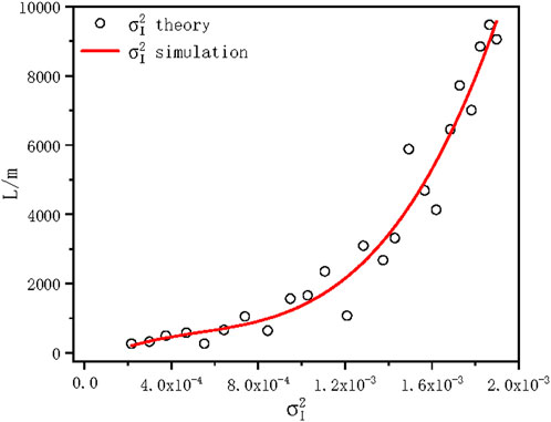
Figure 12. Comparison between the average value and theoretical values of the scintillation index of a Gaussian beam propagating vertically at 10000 m for modified Von Karman turbulence.

It is obvious that as the distance of laser beam transmission in the atmosphere increases, it is increasingly affected by turbulence. The scintillation index of the Gaussian beam simulated fluctuates around the theoretical value, therefore, the simulated scintillation index has a certain consistency with the theoretical value, indicating that the reliability and rationality of the “multi phase screen” method in simulating laser propagation in turbulent atmosphere.

4 Experiment results and analysis

4.1 Mie-Scattering Lidar system

We have designed a Mie-scattering lidar system for detecting atmospheric turbulence based on system simulation parameter results and residual light intensity scintillation theory. The lidar includes laser emission system, receiving system, spectroscopic system and data acquisition system. The laser emission system emits a laser beam, the receiving system receives return signals generated jointly by aerosol scattering effects, and atmospheric turbulence effects, etc., the spectroscopic system separates signals of various wavelengths, and the data acquisition system can amplify and filter the echo signal for display. The schematic diagram and actual Mie-scattering lidar system are shown in Figures 13, 14, respectively.

Figure 13

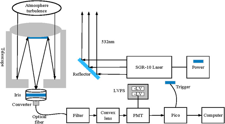
Figure 13. Schematic diagram of Mie-scattering lidar system.

Figure 14

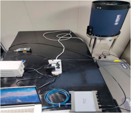
Figure 14. The actual Mie-scattering lidar system used in the experiment.

The system uses a power SGR-10 pulse laser as the laser source, emitting a pulse laser at wavelength of 532 nm with the pulse frequency of 10 Hz. After transmitted into the atmosphere, the laser interacts with molecules and particles in the atmosphere, as well as atmospheric turbulence, to generate a backscattered return signal, which is received by a large aperture telescope, filtered by a small aperture, and then is converged and enters a optical fiber. Through optical fiber, the return signal is incident into the spectroscopic system, and is detected by a photomultiplier tube (PMT). The PMT converts the received optical signal into an electrical signal, which is amplified by an amplifier and sent to the data acquisition and processing system. Figure 15 shows the actual structure of a spectroscopic system, which includes a iris diaphragm, a 532 nm filter, a convex lens, and a PMT. Table 1 lists the main parameters of Mie-scattering lidar for detecting atmospheric turbulence.

Figure 15

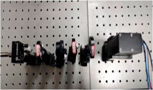
Figure 15. Actual structure of spectroscopic system.

Table 1

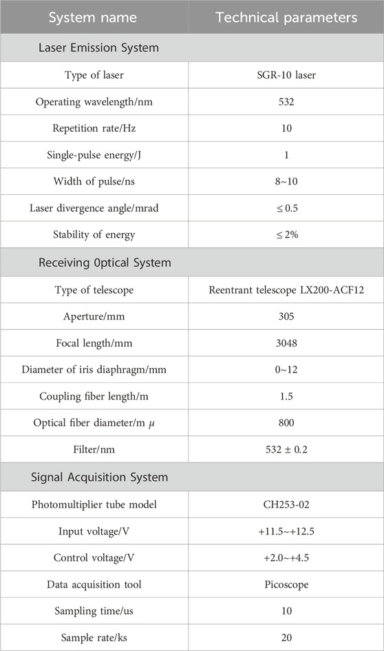
Table 1. Main parameters of Mie-scattering lidar for detecting atmospheric turbulence.

4.2 Measurement results and analysis

When detecting atmospheric turbulence, the Mie-scattering lidar can be regarded as weak fluctuation, the emitted Gaussian beam can be approximately regarded as spherical wave, and the light wave propagation belongs to the turbulence inertial region propagation. In this paper, based on the guidance for simulation analysis, a Mie-scattering lidar system for detecting the intensity of atmospheric turbulence is developed at North Minzu University (106°06′E, 38°29′N) in Yinchuan area, and some experiments were carried out for verifying the atmospheric turbulence detection ability by Mie-Scattering Lidar using modified Von Karman turbulence power Spectrum.

For the modified Von Karman and Kolmogorov turbulent power spectrum, on the path from z = 0 to z = L, the axial scintillation index of spherical waves under the weak fluctuation condition are expressed as in Eqs 18–19, respectively [23]:

$\begin{array}{l}{\sigma }_I^2\left(L\right)=4{\sigma }_{\chi }^2\left(L\right)=\frac{-7.56k^{7/6}\cdot \exp \left({\kappa }_0^2/{\kappa }_m^2\right)}{{\kappa }_m^{5/3}}\\ {\int }_0^L{C}_n^2\left(z\right)\left\{{\left[{\left(\frac{z\left(L-z\right)}{L}\right)}^2\cdot {\kappa }_m^4+k^2\right]}^{5/12}-2k^{5/6}\right\}dz\end{array}(18)$

${\sigma }_I^2\left(L\right)=4{\sigma }_{\chi }^2\left(L\right)=2.25k^{7/6}{\int }_0^L{C}_n^2\left(z\right){\left[\frac{z\left(L-z\right)}{L}\right]}^{5/6}dz(19)$

where, $\kappa$ is space wave number.

Because the measured values in the experiment are generally voltage signals, and the voltage $U$ is proportional to the light intensity $I$, the scintillation index can be converted into voltage form, namely in Eq. 20, [24]:

${\sigma }_I^2={\sigma }_U^2=\frac{〈U^2〉-{〈U〉}^2}{{〈U〉}^2}(20)$

where $〈〉$ represents the ensemble average of light intensity.

In summary, the methods for detecting atmospheric turbulence information adopted in this paper are as follows: Based on the scintillation theory of residual light intensity, the scintillation index at each distance of return signal is obtained according to Eq. 20. Then, according to Eqs 18, 19, the variation trend between the scintillation index and the structure constant of atmospheric refractive index along the propagation path at a certain time is obtained by inversion, and the atmospheric turbulence profile can be obtained.

Figure 16 shows the scintillation index profile at different weather conditions. Here, the height resolution is 44 m and the diameter of iris diaphragm is $d_0=0.9mm$. On 9 August 2023, the weather was sunny and the temperature was higher; On 7 August 2023, the weather was cloudy, with low temperatures and thicker clouds.

Figure 16

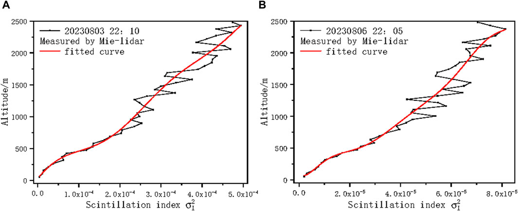
Figure 16. The scintillation index profile under different weather conditions (A) on sunny day (B) on cloudy day.

From Figure 16, the scintillation index basically conforms to the trend of gradually increasing with the increase of height, which is consistent with the scintillation index characteristics and simulation results. In combination with the scintillation index profile obtained in Figure 16, the modified Von Karman turbulence profile under two different weather conditions is calculated by Newton iteration method, as shown in Figure 17.

Figure 17

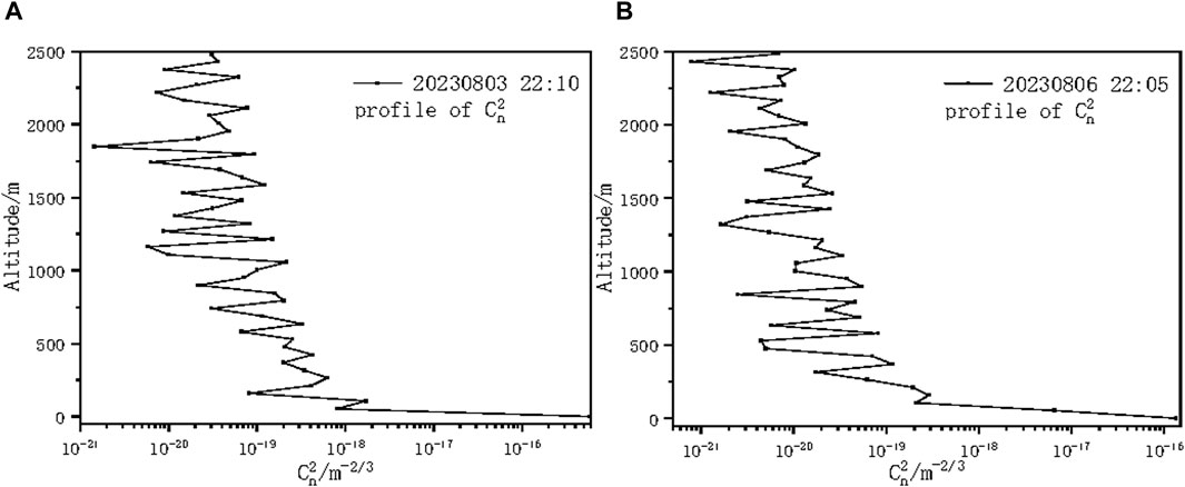
Figure 17. The inverted Modified Von Karman turbulence intensity profiles under different weather conditions (A) on sunny day (B) on cloudy day.

From Figure 17, the modified Von Karman turbulence profile derived also fluctuates randomly with height. The turbulence intensity at high is small and belongs to weak turbulence according to the order of magnitude. The scintillation index and turbulence intensity under cloudy day are significantly lower than those under sunny day, and the modified Von Karman turbulence intensity is about one order of magnitude smaller on cloudy day than under sunny day. This is because the random fluctuation of atmospheric temperature is the main reason for the random fluctuation of atmospheric refractive index, and the temperature fluctuation on cloudy day is lower than that on sunny day. In fact, on sunny day, the sunlight radiation on the ground makes the temperature rise continuously, and the heat is transported upward, so that the temperature fluctuation is enhanced and the turbulence effect is significant.

In experiment, when the diameter of iris diaphragm of d₀ is selected as 1.2, 0.9, and 0.5 mm, respectively, the scintillation index and atmospheric refractive index structure constant of modified Von Karman turbulence profile on the 3 days were detected and calculated, respectively, which is shown in Figure 18 and Figure 19. On the 3 days, the weather conditions were basically the same, namely, cloudless and the wind was light.

Figure 18

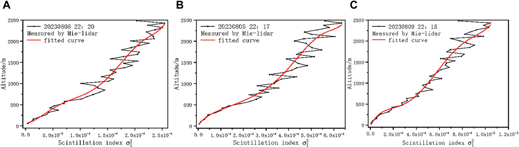
Figure 18. The scintillation index profiles at different diameter of iris diaphragm (A) at d₀ = 1.2 mm (B) at d₀ = 0.9 mm (C) at d₀ = 0.5 mm.

Figure 19

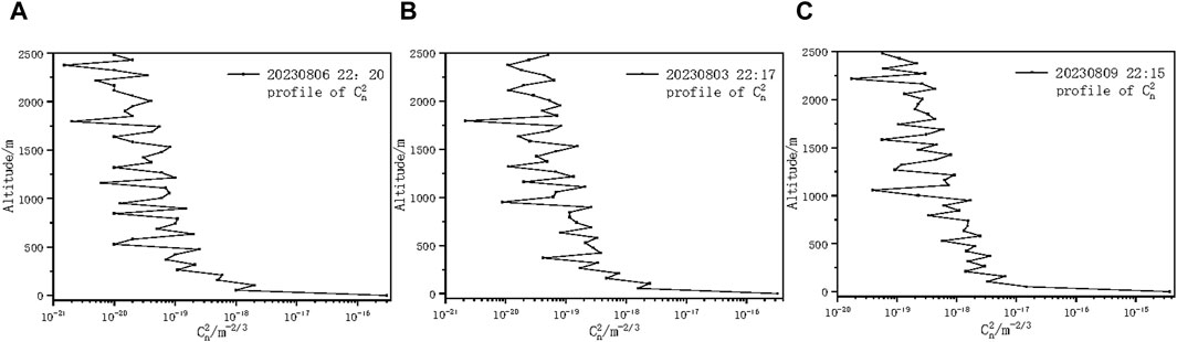
Figure 19. The modified Von Karman turbulence intensity profile on the 3 days with different diameter of iris diaphragm (A) at d₀ = 1.2 mm (B) at d₀ = 0.9 mm (C) at d₀ = 0.5 mm.

As can be seen from Figure 18, the smaller diameter of iris diaphragm, the larger the resulting scintillation index. It is due to the aperture smoothing effect, the increase of aperture will cause the generation of uncorrelated light intensity fluctuation regions, and because the uncorrelated elements will cancel each other, the overall scintillation will be weakened, and eventually the obtained scintillation index will be small. Figure 19 also shows that the smaller diameter of iris diaphragm, the greater the modified Von Karman turbulence intensity obtained by inversion.

In Figure 19, the atmospheric refractive structure constant $C_n^2$ profiles have fluctuations, and a relatively weak turbulent layer appears at about 350 m. This is because there is a temperature inversion layer at 350 m, these $C_n^2$ profiles have a tendency to decrease rapidly. Overall, these $C_n^2$ profiles decrease with the increase of detection height, which meets the characteristics of strong turbulence in the lower layer and weak turbulence in the upper layer.

For verifying the feasibility of detection result atmosphere turbulence by Mie-scattering lidar, the Hufnagel-Valley model [25] is selected and modified to conform to the nighttime meteorological conditions in Yinchuan area. The $C_n^2$ profile model conforming to Yinchuan area was fitted accordingly, and the model formula was shown as in Eq. 21

$C_n^2\left(h\right)=3.12\times {10}^{-55}{h}^{10}{e}^{-h/1000}+2.23\times {10}^{-18}{e}^{-h/1500}+4.31\times {10}^{-17}{e}^{-h/100}(21)$

The wavelength of the laser emitted by the Mie-scattering lidar is 532 nm, the frequency is 10 Hz, the diameter of iris diaphragm is d₀ = 0.5 mm, and the weather on the experiment day is clear and windless. The modified Von Karman turbulence and Kolmogorov turbulence intensity were detected, respectively, and the corresponding turbulence profiles obtained by inversion were compared with Hufnagel-Valley model in Yinchuan area. Figure 20 shows the comparison result.

Figure 20

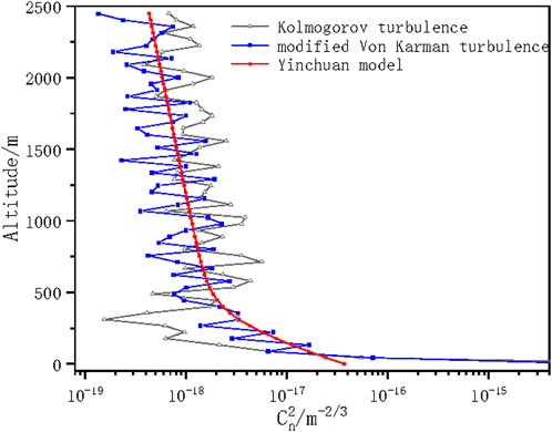
Figure 20. The comparison of atmospheric turbulence profile detected by the Mie-scattering lidar with Hufnagel-Valley in Yinchuan area.

Through comparison, it can be seen that the overall change trend of atmospheric turbulence profile detected by the Mie-scattering lidar is in line with the change trend of Hufnagel-Valley model in Yinchuan area. The $C_n^2$ in the low altitude area decreases rapidly with the increase of height, and the $C_n^2$ in the high altitude area decreases gradually with the increase of height. The modified Von Karman turbulence profile and Kolmogorov turbulence profile both show such a trend. Compared with the Hufnagel-Valley model in Yinchuan area, the modified Von Karman turbulence profile is more consistent with the actual situation, while the Kolmogorov turbulence profile is one order of magnitude smaller than the actual situation at low height. However, in the upper height, the detection results fluctuate around the theoretical values.

In general, the detection results are distributed near the theoretical model, indicating that the detection of atmospheric turbulence $C_n^2$ profile by the Mie-scattering lidar is feasible.

5 Conclusion

This study is based on the modified Von Karman turbulence model. FFT method is used for numerical simulation, and Zernike polynomial is used as low-frequency compensation to generate the modified Von Karman turbulence phase screen. At the same time, the parameters of phase screen size, spacing and atmospheric turbulence intensity are changed, and their effects on the simulation results are discussed. The phase structure function before and after compensation is compared with the theoretical value, and the result shows that the phase structure function generated after compensation is closer to the theoretical curve. At the same time, the propagation of Gaussian beam from Mie-scattering lidar on the vertical path is simulated numerically. The results show that the modified Von Karman turbulence has a great effect on the propagation of Gaussian beam. When the Gaussian beam passes through the modified Von Karman turbulence, the stronger the turbulence intensity, the larger the phase screen distance, the greater the beam dispersion degree, and the scintillation index is in good agreement with the theoretical value.

Moreover, based on the guidance for simulation analysis, a Mie-scattering lidar system for detecting the atmospheric turbulence intensity was developed and the vertical direction of atmospheric turbulence was detected. The scintillation index profile was calculated by the received light intensity, and then the $C_n^2$ profile of atmospheric turbulence under different weather conditions was obtained by Newton iteration method. The influence of different conditions on the atmospheric turbulence profile was analyzed by changing the relevant parameters. The detected atmospheric turbulence intensity profile was basically consistent with the trend of Hufnagel-Valley model in Yinchuan area. In general, it is feasible for detecting the modified Von Karman turbulence profile using the Mie-scattering lidar.

Data availability statement

The raw data supporting the conclusion of this article will be made available by the authors, without undue reservation.

Author contributions

LZ: Investigation, Software, Writing–original draft. JM: Conceptualization, Funding acquisition, Methodology, Project administration, Supervision, Writing–review and editing.

Funding

The author(s) declare financial support was received for the research, authorship, and/or publication of this article. This work was supported by the National Natural Science Foundation of China (No. 42265009), the Natural Science Foundation of Ningxia Province (No. 2021AAC02021), the Innovation Team of Lidar Atmosphere Remote Sensing of Ningxia Province, the high-level talent selection and training plan of North Minzu University, the special funds for basic scientific research business expenses of central universities of North Minzu University (No. FWNX20), and the Ningxia First-Class Discipline and Scientific Research Projects (Electronic Science and Technology) (No. NXYLXK2017A07).

Conflict of interest

The authors declare that the research was conducted in the absence of any commercial or financial relationships that could be construed as a potential conflict of interest.

Publisher’s note

All claims expressed in this article are solely those of the authors and do not necessarily represent those of their affiliated organizations, or those of the publisher, the editors and the reviewers. Any product that may be evaluated in this article, or claim that may be made by its manufacturer, is not guaranteed or endorsed by the publisher.

References

1. Karman VT. Progress in the statistical theory of turbulence. Proc Natl Acad ences USA (1948) 34(11):530–9. doi:10.1073/pnas.34.11.530

CrossRef Full Text | Google Scholar

2. Li YQ, Wu ZS, Zhang YY, Wang MJ. Scintillation of partially coherent Gaussian—Schell model beam propagation in slant atmospheric turbulence considering inner-and outer-scale effects. Chin Phys B (2014) 23(7):074202. doi:10.1088/1674-1056/23/7/074202

CrossRef Full Text | Google Scholar

3. Gracheva ME, Gurvich AS. Strong fluctuations in the intensity of light propagated through the atmosphere close to the earth. Soviet Radiophysics (1965) 8(4):511–5. doi:10.1007/bf01038327

CrossRef Full Text | Google Scholar

4. Wu W, Ning Y, Ren Y, Wu Y, Shu B. Research progress of scintillations for laser array beams in atmospheric turbulence. Prog Laser Optoelectronics (2012) 49(07):070008. doi:10.3788/LOP49.070008

CrossRef Full Text | Google Scholar

5. Cui G, Ren Z, Chen C. The experiment of a system for measurements of the refractive index structure constant along a 1 km free-space laser propagation path. In: 2012 International Conference on Optoelectronics and Microelectronics. IEEE (2012). p. 313–8.

CrossRef Full Text | Google Scholar

6. Tan Z, Ke X. The variance of angle-of-arrival fluctuation of partially coherent Gaussian-Schell Model beam propagations in slant atmospheric turbulence. In: AOPC 2017: Fiber Optic Sensing and Optical Communications. Beijing: SPIE (2017). p. 297–305. doi:10.1117/12.2285126

CrossRef Full Text | Google Scholar

7. Jia R, Wei H, Zhang H, Cheng L, Cai D. Scintillation index of echo wave in slant atmospheric turbulence. Optik - Int J Light Electron Opt (2015) 126(24):5122–6. doi:10.1016/j.ijleo.2015.09.166

CrossRef Full Text | Google Scholar

8. Chen Z, Cui S, Zhang L, Sun C, ong M, Pu J. Measuring the intensity fluctuation of partially coherent radially polarized beams in atmospheric turbulence. Opt Express (2014) 22(15):18278–83. doi:10.1364/oe.22.018278

PubMed Abstract | CrossRef Full Text | Google Scholar

9. Zhu L. Research of atmosphere turbulence simulation in free space optical communication. Beijing: Master Dissertation of Beijing University of Posts and Telecommunications (2016). 1: 14-18, 53-76.

Google Scholar

10. Wang H, Li y, Cao M, Peng Q. Experimental Investigation of Light Intensity Distribution and Fluctuation Characteristics in Lanzhou Area. Acta Photonica Sinica (2017) 46(06):0601002. doi:10.3788/gzxb20174606.0601002

CrossRef Full Text | Google Scholar

11. Aly AM, Fayed HA, Ismail NE, Aly MH. Plane wave scintillation index in slant path atmospheric turbulence: closed form expressions for uplink and downlink. Opt Quan Electron (2020) 52:350–14. doi:10.1007/s11082-020-02463-w

CrossRef Full Text | Google Scholar

12. Fei W, Jia-Yi Y, Xian-Long L, Yang-Jian C. Research progress of partially coherent beams propagation in turbulent atmosphere. Acta Physica Sinica (2018) 67(18):184203. doi:10.7498/aps.67.20180877

CrossRef Full Text | Google Scholar

13. Mert B. Properties of hyperbolic sinusoidal Gaussian beam propagating through strong atmospheric turbulence. Microwave Opt Technol Lett (2021) 63(5):1595–600. doi:10.1002/mop.32799

CrossRef Full Text | Google Scholar

14. Wu J, Ke X, Yang S, Ding D. Effect of multi-beam propagation on free-space coherent optical communications in a slant atmospheric turbulence. J Opt (2022) 24(7):075601. doi:10.1088/2040-8986/ac6cf6

CrossRef Full Text | Google Scholar

15. Rao R. Propagation of light in turbulent atmosphere. Hefei: Anhui Science and Technology Press (2005).

Google Scholar

16. He C, Shen Y, Forbes A. Towards higher-dimensional structured light. Light Sci Appl (2022) 205:205. doi:10.1038/s41377-022-00897-3

PubMed Abstract | CrossRef Full Text | Google Scholar

17. Chen Z, Cui S, Zhang L, Sun C, Xiong M, Pu J. Experimental measurement of scintillation index of vortex beams propagating in turbulent atmosphere. Optoelectronics Lett (2015) 11(2):141–4. doi:10.1007/s11801-015-4187-y

CrossRef Full Text | Google Scholar

18. Guan K. The aberration of OAM beams in atmosphere turbulence and compensation methods research. Harbin: Harbin Institute of Technology (2018). p. 31–44.

Google Scholar

19. Geng S. Study on propagation and target echo characteristics of partially coherent vortex beam in atmospheric turbulence. Xi'an: Xidian University (2021). p. 36–7. doi:10.27389/d.cnki.gxadu.2021.002186

CrossRef Full Text | Google Scholar

20. Arguelles AP. Von Karman spatial correlation function to describe wave propagation in polycrystalline media. J Appl Phys (2022) 131(22):131. doi:10.1063/5.0091521

CrossRef Full Text | Google Scholar

21. Nape I, Sephton B, Ornelas P, Moodley C, Forbes A. Quantum structured light in high dimensions. APL Photon (2023) 8(5). doi:10.1063/5.0138224

CrossRef Full Text | Google Scholar

22. Zhang Y. Study on propagation on properties of array beams in atmospheric turbulence in FSO system. Xi'an: Master Dissertation of Xi'an University of Technology (2017). p. 44–56.

Google Scholar

23. Huang H. Effect of near-Earth atmospheric turbulence on amplitude fluctuation characteristics of laser transmission signal [D]. Nanjing:Master Dissertation of Nanjing University of Science and Technology (2012):16–34.

Google Scholar

24. Fu S, Gao C. Influences of atmospheric turbulence effects on the orbital angular momentum spectra of vortex beams. Photon Res (2016) 4(5):B1. doi:10.1364/prj.4.0000b1

CrossRef Full Text | Google Scholar

25. Rao R. Light propagation in the turbulent atmosphere. Hefei, China: Anhui Science and Technology Press (2005). p. 4–5.

Google Scholar