Effect of network architecture on physics-informed deep learning of the Reynolds-averaged turbulent flow field around cylinders without training data

1 Introduction

Neural networks (NNs) can be used to approximate arbitrary nonlinear function and its derivatives [20]. However, deep learning (DL) requires large data sets to train these networks [28]. Physics-informed neural networks (PINNs) have attracted a growing interest, as the required amount of training data can be significantly reduced by deploying physics-informed DL. PINNs are NNs that are trained to respect given laws of physics by utilizing a composed loss function that considers residuals of the underlying physics equations and boundary conditions. Physics-informed DL has been demonstrated by Lagaris et al. [13] who used PINNs to solve different differential equations. Later, Raissi et al. [22–24] extended this research further and trained several partial differential equations without relying on training data. These studies proved the effectiveness of PINNs and motivated a growing number of investigations in all fields of computational physics.

In the field of fluid dynamics, a variety of research has been carried out. Many investigations focused on laminar flows at low Reynolds numbers [9, 14, 18, 25, 27]. Several investigations covered turbulent flows at high Reynolds numbers, and PINNs were trained to solve the Reynolds-averaged Navier-Stokes (RANS) equations. High Reynolds number flows are important research objects for physics-informed DL as most technical flows are subject to high Reynolds numbers and additional turbulence modeling equations, strong convection, as well as high gradients impose challenges to the training success. RANS solutions obtained by PINNs could be applied to surrogate modeling [6] or optimization problems [7] to replace traditional computational fluid dynamics (CFD) calculations of the RANS equations. Several RANS-PINN studies have been conducted for high Reynolds number flows incorporating turbulence models such as Prandtl’s mixing length model [7, 21], the k-ϵ model [5], the k-ω model [21], the Spalart-Allmaras (SA) model [19], as well as equation-free modeling approaches [3, 21, 36]. This encouraging research, which demonstrated the capabilities of PINNs, incorporated labeled training data into the training routine of the PINN [5, 19, 21, 36], trained parts of the complete flow field using unsupervised DL [3, 36], or trained flows without separation without using training data [7]. Hence, the evaluation of unsupervised physics-informed DL methods applied to complete flow fields featuring flow separation at elevated Reynolds numbers remains an open question.

Rao et al. [26] presented a mixed-variable approach of superior accuracy for a low Reynolds number flow around a cylinder without using training data. Motivated by their results, we evaluated the unsupervised mixed-variable method applied to a high Reynolds number flow considering RANS turbulence modeling. To conduct a comparative study, we trained several PINNs to predict the two-dimensional Reynolds-averaged turbulent flow field around two cylinders. We compared the mixed-variable method to traditional PINNs and evaluated various network architectures to identify the most accurate network shape and size. We used the PINNs to solve the RANS equations and applied Prandtl’s mixing length model to model turbulence. The PINN predictions were compared with CFD results as well as experimental measurements. To our knowledge, this is the first detailed report of unsupervised physics-informed DL learning of the RANS equations for a complete flow field featuring flow separation at an elevated Reynolds number. The motivation of this work was to explore and evaluate unsupervised DL methods and network architectures with respect to their prediction accuracy of Reynolds-averaged flows when no training data are provided.

2 Materials and methods

2.1 Geometry

We investigated the two-dimensional flow around a circular cylinder as well as a square cylinder. Figure 1 illustrates the cylinder geometries. We considered a fluid with a density ρ of 1 kg/m³ and an inlet velocity of 1 m/s. Dimensions and inlet velocity were chosen to yield a scaled problem with network inputs and outputs ranging between −1 and +1 as closely as possible. The resulting flow fields featured important phenomena, such as stagnation points, high gradient boundary layers, flow separation, and wakes. The two geometries exemplified curved and cornered obstacles that impose different flow separation mechanisms triggered at the rounded or cornered walls. We employed three different versions of the cylinder geometries as presented in Table 1. Geometries G1 and G2 were used to evaluate the effect of network architecture, network shape, and PINN methods for different cylinder shapes at an elevated Reynolds number. The large scale of the cylinders allowed more accurate and spatially detailed PINN predictions. This set up represented a channel flow and allowed comparison to a PINN study of Rao et al. [26]. Geometry G3 was selected to facilitate a comparison of the PINN method with the experimental results of Lyn et al. [17] as well as a PINN study of Ang et al. [1]. Due to the small scale of the square cylinder, blockage ratio effects of geometry G3 were negligibly small; however, the spatial accuracy of the PINN method was reduced.

Figure 1

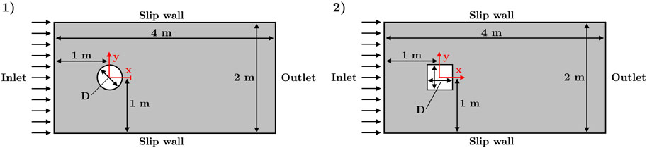
Figure 1. Geometries of the circular cylinder (left) and the square cylinder (right).

Table 1

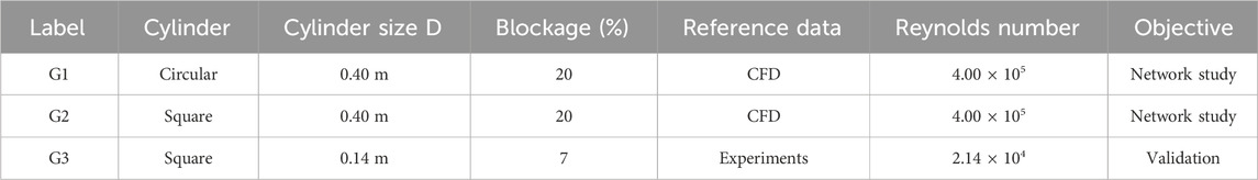
Table 1. Parameters of the investigated geometries.

2.2 Governing equations and PINN method

The associated flow field is governed by the continuity Eq 1 and the two-dimensional incompressible Reynolds-averaged Navier-Stokes Eq. 2

$\frac{\partial \overline{u_i}}{\partial xi}=0(1)$

$\overline{u_j}\frac{\partial \overline{u_i}}{\partial x_j}+\overline{u_j^{\prime }\frac{\partial u_i^{\prime }}{\partial x_j}}=-\frac{1}{\rho }\frac{\partial \bar{p}}{\partial x_i}+\frac{\mu }{\rho }\frac{{\partial }^2\overline{u_i}}{\partial x_j\partial x_j}(2)$

with Reynolds-averaged velocities and pressure $\overline{u_i}$, $\overline{u_j}$, and $\bar{p}$, constant density ρ, and constant dynamic viscosity μ. In the RANS equations, the second order moments of the turbulent velocity fluctuations, $u_i^{\prime }$, and $u_j^{\prime }$, represent the Reynolds stresses ${\tau }_{ij}^{\prime }$

$\frac{\partial {\tau }_{ij}^{\prime }}{\partial x_j}=\overline{u_j^{\prime }\frac{\partial u_i^{\prime }}{\partial x_j}}(3)$

The Reynolds stresses are modeled using the Boussinesq hypothesis

${\tau }_{ij}^{\prime }=-\overline{u_i^{\prime }{u}_j^{\prime }}=\frac{{\mu }_t}{\rho }\left(\frac{\partial \overline{u_i}}{\partial x_j}+\frac{\partial \overline{u_j}}{\partial x_i}\right)-\frac{2}{3}k{\delta }_{ij}(4)$

where μ_t is a turbulent viscosity representing the effects of the turbulent eddies on the mean flow, k is the turbulent kinetic energy, and δ_ij is the Kronecker delta. The approach of modeling turbulence via an eddy viscosity is based on the gradient diffusion hypothesis and, hence, assumes an alignment of the turbulent transport with the negative gradient of the mean flow. The application of an isotropic turbulent viscosity, μ_t, facilitates modeling of turbulent stresses in the same way as viscous stresses. A turbulence model is required to calculate the turbulent viscosity. Here, Prandtl’s mixing-length model was selected as applied in [7] due to its stability and robustness. For this model, the turbulent viscosity is estimated using a mixing length, l_m, that represents the size of the characteristic eddies as follows:

${\mu }_t=\rho l_m^2\sqrt{S}(5)$

where S represents the modulus of the mean rate of strain tensor. For the two-dimensional flow considered here, S reads

$S=2{\left(\frac{\partial \bar{u}}{\partial x}\right)}^2+2{\left(\frac{\partial \bar{v}}{\partial y}\right)}^2+{\left(\frac{\partial \bar{u}}{\partial y}+\frac{\partial \bar{v}}{\partial x}\right)}^2(6)$

The mixing length l_m is calculated as follows:

$l_m=\mathrm{m}\mathrm{i}\mathrm{n}\left(\kappa d,0.09d_{\mathit{max}}\right)(7)$

where d is the distance from the wall, κ ≈ 0.4 is the von Kármán constant, and d_max is a characteristic maximal length scale, here taken as the maximum wall distance of 1.0 m. Using the eddy viscosity approach, a resulting viscosity, μ_res, is calculated and deployed in the RANS equations

${\mu }_{\mathit{res}}=\mu +{\mu }_t(8)$

Two physics-informed DL methods were compared. The corresponding models were trained by minimizing a composed loss function $\mathcal{L}(\theta )$:

$\mathcal{L}\left(\theta \right)={\mathcal{L}}_b\left(\theta \right)+{\mathcal{L}}_e\left(\theta \right)(9)$

where ${\mathcal{L}}_b$ is the loss on the boundary conditions, and ${\mathcal{L}}_e$ is the loss for the RANS equations. The individual loss terms were calculated using the mean squared error:

${\mathcal{L}}_b=\frac{1}{N_b}\sum _{n=1}^{N_b}|{\mathbf{U}}_b^n-{\tilde{\mathbf{U}}}_b^n{|}^2(10)$

${\mathcal{L}}_e=\frac{1}{N_e}\sum _{k=1}^3\sum _{n=1}^{N_e}|{\epsilon }_k^n{|}^2(11)$

where N_b and N_e represent the number of points for which the boundary conditions and RANS equations were trained. ${\mathbf{U}}_b^n=[u_b^n,v_b^n]$ are the given velocity and pressure conditions for points n on the boundaries. ${\tilde{\mathbf{U}}}_b^n$ and ${\tilde{\mathbf{U}}}_d^n$ represent the output of the PINN at the corresponding training points and ${\epsilon }_k^n$ is the residual of the kth equation at point n.

For the first method, a traditional PINN was trained to predict the Reynolds-averaged velocity and pressure fields. The PINN reads as follows:

${NN}_{\theta }\left(\begin{array}{c}\hfill x\hfill \\ \hfill y\hfill \end{array}\right)=\left(\begin{array}{c}\hfill u\hfill \\ \hfill v\hfill \\ \hfill p\hfill \end{array}\right)(12)$

where θ are the trainable parameters (weights and biases) of the NN. Hence, for the traditional PINN approach, the model maps the input coordinates x and y to the output solution field components u, v, and p. The Navier-Stokes Eqs 1, 2 were used as the residual functions as follows:

${\epsilon }_{k=1}=\frac{\partial \overline{u_i}}{\partial xi}(13)$

${\epsilon }_{k=\mathrm{2,3}}=\overline{u_j}\frac{\partial \overline{u_i}}{\partial x_j}+\frac{1}{\rho }\frac{\partial \bar{p}}{\partial x_i}-\frac{{\mu }_{\mathit{res}}}{\rho }\frac{{\partial }^2\overline{u_i}}{\partial x_j\partial x_j}(14)$

For the second method, a mixed-variable approach as presented by Rao et al. [26] provided a system of equation that can be learned more easily by the PINN. The correspondingly simplified RANS equations read as follows:

$\overline{u_j}\frac{\partial \overline{u_i}}{\partial x_j}=\frac{1}{\rho }\frac{\partial {\sigma }_{ij}}{\partial x_j}(15)$

Using this method, the stress tensor σ_ij is utilized

${\sigma }_{ij}=-p{\delta }_{ij}+{\mu }_{\mathit{res}}\left(\frac{\partial \overline{u_i}}{\partial x_j}+\frac{\partial \overline{u_j}}{\partial x_i}\right)(16)$

The pressure p can be calculated as the trace of σ

$p=-\frac{1}{2}{\sigma }_{ii}(17)$

As suggested by Rao et al. [26], the stream variable ψ was used to represent the velocity field. This automatically satisfies the continuity Eq 1 and amplified the learning success of the NN. The velocity components can be retrieved using

$\left(\begin{array}{c}\hfill u\hfill \\ \hfill v\hfill \\ \hfill 0\hfill \end{array}\right)=\nabla \times \left(\begin{array}{c}\hfill 0\hfill \\ \hfill 0\hfill \\ \hfill \psi \hfill \end{array}\right)(18)$

where ∇ is the Nabla operator. A feedforward NN was trained to predict ψ, p, and the stress components σ_xx, σ_xy = σ_yx, and σ_yy. The network takes the coordinates x and y as inputs and passes the velocity components, the pressure, and the stress components back. The model reads as follows:

${NN}_{\theta }\left(\begin{array}{c}\hfill x\hfill \\ \hfill y\hfill \end{array}\right)=\left(\begin{array}{c}\hfill \psi \hfill \\ \hfill p\hfill \\ \hfill {\sigma }_{xx}\hfill \\ \hfill {\sigma }_{xy}\hfill \\ \hfill {\sigma }_{yy}\hfill \end{array}\right)(19)$

In agreement with Eqs 15–17, the residuals ɛ_k are computed as

${\epsilon }_{k=\mathrm{1,2}}=\overline{u_j}\frac{\partial \overline{u_i}}{\partial x_j}-\frac{\partial {\sigma }_{ij}}{\partial x_j}(20)$

${\epsilon }_{k=\mathrm{3,4,5}}=-p+{\mu }_{\mathit{res}}\left(\frac{\partial \overline{u_i}}{\partial x_j}+\frac{\partial \overline{u_j}}{\partial x_i}\right)-{\sigma }_{ij}(21)$

${\epsilon }_{k=6}=p+\frac{1}{2}{\sigma }_{ii}(22)$

For the traditional approach, the two input neurons were fed into a single fully connected feed-forward network with three output neurons as determined by Eq 12. For the mixed-variable approach, the two input neurons were fed into a single fully connected feed-forward network with five output neurons as defined by Eq 19. Figure 2 shows the two methods that were compared here.

Figure 2

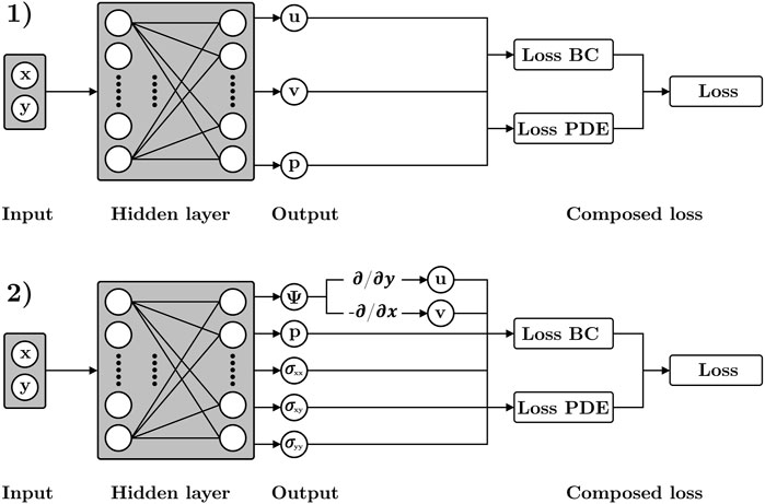
Figure 2. Tested physics-informed deep learning methods. 1) Traditional fully-connected feed-forward architecture; 2) Mixed-variable fully connected feed-forward architecture.

For all networks, a tanh activation function was deployed. In a first step, the PINNs were trained using the Adam optimizer for 100,000 iterations with a decaying learning rate. The initial learning rate was set to 0.001 and was reduced by a factor of 0.9 every 2,000 iterations. In a second step, the models were trained using the L-BFGS optimizer under the predefined default settings. No loss weigthing factors were defined. The training was conducted using the tensorflow-based library DeepXDE [16] on a 16 GB NVIDIA Quadro RTX 5000.

2.3 Reference data

The capability of the PINN to represent the solution of the RANS equations under consideration of the mixing length model was evaluated and compared with CFD simulations for geometries G1 and G2. For the CFD calculations, the element-based finite volume flow solver MAYA included in the Simcenter software was used. The MAYA solver provided the mixing length model with Van Driest damping. Unstructured meshes featuring prism layers on the cylinders were defined. The second order upwind discretization scheme was deployed. The incompressible calculations were carried out until reaching the minimal achievable residuals. A grid sensitivity analysis was carried out to verify the models. For the grid study, three grids were generated using a refinement factor of 1.3. Excellent agreement between all three grids was found and, consequently, the reference solution was concluded to be grid independent.

The PINN predictions for geometry G3 were compared with experimental results of Lyn et al. [17] who conducted two-component laser-Doppler measurements for a square cylinder inside a closed water channel at a Reynolds number of 2.14 × 10⁴. The time averaged data were obtained from the ERCOFTAC validation database [4].

2.4 Study design

This study, comprising three parts, compared the traditional method with the mixed-variable method, investigated effects of network shape and size for different geometries, and compared the predictions with measurements. For both PINN methods, several network architectures were compared. The network sizes were chosen to yield the same number N_θ of trainable parameters θ (weights and biases) inside the network, where N_θ is defined as follows:

$N_{\theta }=N_{in}{N}_n+N_n^2\left(N_l-1\right)+N_{\mathit{out}}{N}_n+N_n{N}_l(23)$

Here, N_out represents the number of output neurons and N_in the number of input neurons. The number of neurons per layer, N_n, and the number of hidden layers, N_l, were set to yield a progressing series of shape factor values, λ. The shape factor was defined as follows:

$\lambda =\frac{N_n}{N_l}(24)$

A low value of λ represented a deep but narrow network architecture featuring comparatively few neurons per layer and many hidden layers. An elevated result for λ corresponded to a shallow but wide network consisting of a high amount of neurons per layer and few hidden layers.

In the first part of our study, the traditional method was tested using geometry G1. This part documented limitations of the traditional PINN method when applied to high Reynolds number flows. Table 2 lists the tested networks of the first part. In the second part, the best fitting network shapes and sizes for mixed-variable PINN models were evaluated and the results for geometry G1 and G2 were compared. The purpose of this part was to find appropriate network shapes, outline differences between the two geometries, and document capabilities and limitations of unsupervised mixed-variable models when applied to high Reynolds number flows. A total of five network architectures were deployed with corresponding shape factors ranging from 4.08 × 10⁻¹ to 1.34 × 10². Table 2 lists the evaluated networks. Furthermore, after selecting the network shapes giving the most accurate results, several networks featuring a constant shape factor and a progressing number of trainable parameters θ were defined and tested. Different shape factors were chosen for the circular cylinder and the square cylinder. Table 2 lists the networks evaluated in the second step. 10,000 randomly distributed training points were used on the boundaries as well as inside the flow domain for geometries G1 and G2. This represented 1,250 points per m² of the flow domain and 754 points per m of the boundaries. The number of points was evaluated in a prior sensitivity analysis conducted for the circular cylinder G1 using the mixed-variable PINN N50L30. The evaluation revealed no increase in accuracy by increasing the number of points, as shown in Figure 3. The density of points deployed here was 3.87 times greater than used in a study of Ang et al. [1] who reported no change in accuracy beyond 323 points per m² of the scaled flow domain for a laminar flow field.

Table 2

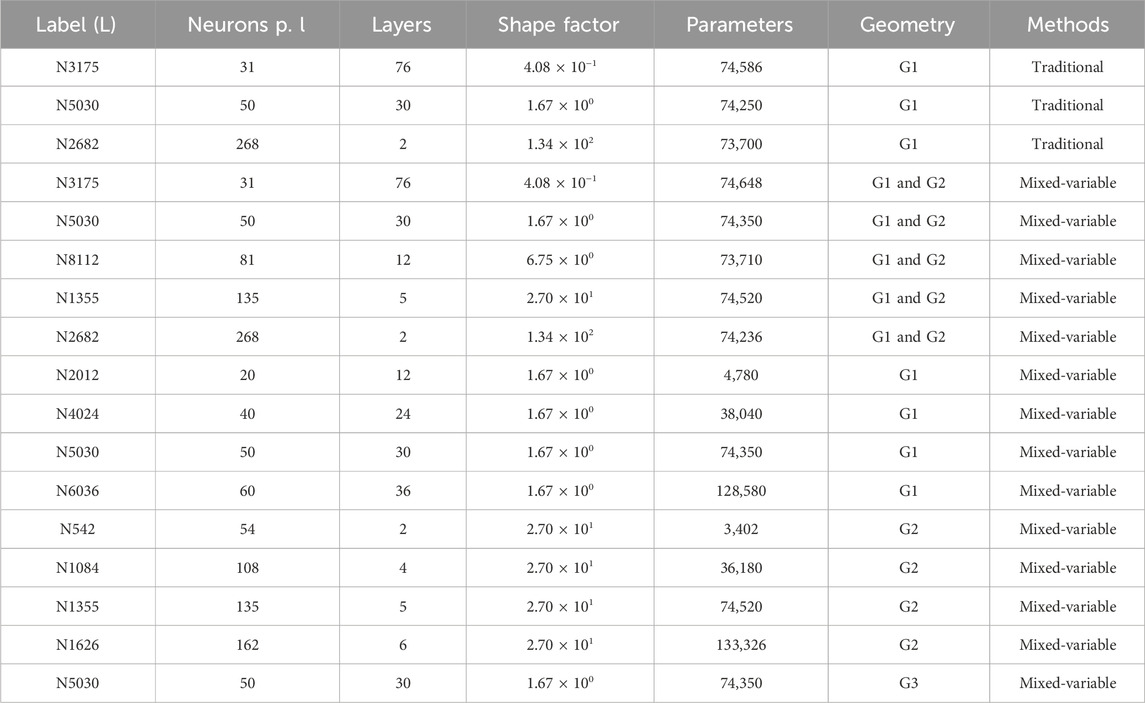
Table 2. Network architectures using the traditional PINN method evaluated in the three parts.

Figure 3

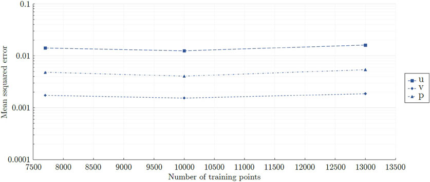
Figure 3. Global mean squared errors obtained for the large scale circular cylinder G1 using different quantities of training points. For visualization purposes, the data points are connected by straight lines.

In the third part, geometry G3 was considered and an unsupervised PINN was compared with the experimental results of Lyn et al. [17]. A search for the most suitable network shape was conducted in the same way as described above for part two. As the general method and behavior of the PINN was equivalent, the detailed results of this study are not presented here. Model N50L30 was identified as the most suitable architecture for geometry G3. The corresponding settings of the network are listed in Table 2. To account for the small scale of the cylindrical body contained in geometry G3, the number of training points inside the domain was increased to 80,000. The purpose of this part was to get an impression of the validity of the mixed-variable PINN method when no labeled training data are provided.

3 Results

3.1 Performance of the traditional method

The traditonal PINNs failed to capture the flow field, independent of network architecture. Figure 4 displays comparative predictions for the velocity field around the circular cylinder. As a reference, the CFD results are shown as well. Several models are exhibited that represent high, moderate, and low shape factors. From the shown models, N31L76 and N268L2 both failed to capture the reference flow field accurately. Model N50L30 provided the best representation of the flow field but the wake length was overestimated and the velocity of the high speed region at the lateral sides of the cylinder was underestimated and the region separated from the cylinder wall. Overall, the flow field was not captured accurately by the traditional PINN method, neither quantitatively nor qualitatively.

Figure 4

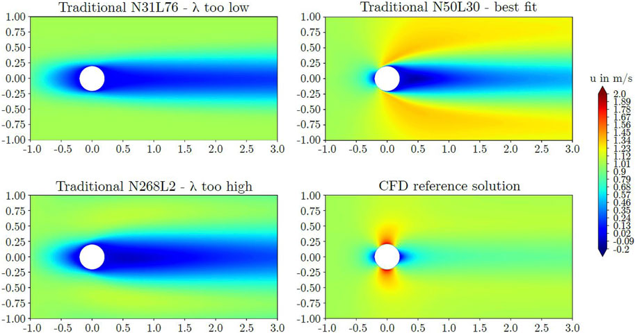
Figure 4. Predicted axial velocities around the circular cylinder obtained by the traditional PINN method.

3.2 Effect of network architecture using the mixed-variable method

The mixed-variable approach was observed to be sensitive to the network shape. Too deep as well as too wide networks failed to capture the flow field. Figures 5, 6 display predicted axial velocities of several models together with comparative CFD data. From the shown models, N31L76 and N268L2 represent low and high shape factors, respectively. Both architectures failed to capture the reference flow field accurately. For the circular cylinder, model N50L30 obtained the most accurate predictions, capturing the stagnation region, the thin boundary layer on the cylinder, as well as the wake. However, the wake length was overestimated compared with the reference solution and the high speed region on the lateral sides of the cylinder was deformed. The length of the wake defined as the downstream distance behind the cylinder until 60% of the inlet velocity was recovered was predicted to be 1.32 m while the reference CFD simulation yielded a wake length of 0.27 m. Correspondingly, the PINN predicted a recirculation length of 0.16 m while the CFD computation featured a shorter recirculation region of 0.02 m. For the square cylinder, model N135L5 exhibited the most accurate results. The stagnation region, the cylinder wake, and the small area of flow separation and recirculation at the lateral sides of the cylinder was captured. However, the size of the low velocity stagnation region upstream of the cylinder was overpredicted when compared with the reference solution. For the square cylinder, the wake length was predicted more accurately by the mixed-variable PINN than for the circular cylinder as the PINN featured a wake length of 2.72 m while the CFD solution gave a length of 2.49 m. The recirculation length as predicted by the PINN was 0.52 m and the reference simulation featured a recirculation length of 0.38 m.

Figure 5

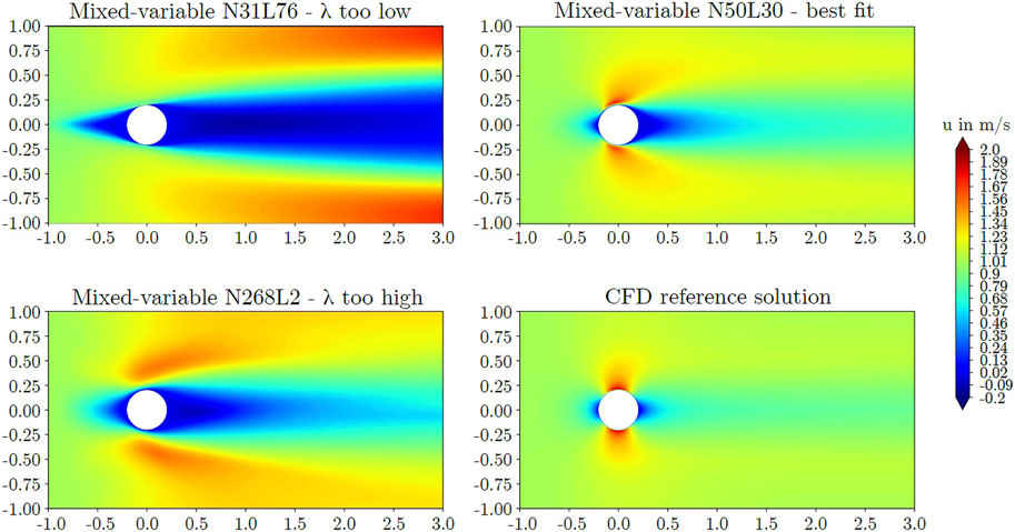
Figure 5. Predicted axial velocities around the circular cylinder obtained from the mixed-variable PINN method.

Figure 6

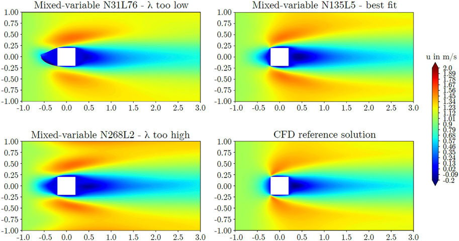
Figure 6. Predicted axial velocities around the square cylinder obtained from the mixed-variable PINN method.

Figure 7 compares axial velocities of the different mixed-variable PINN models with the CFD calculations for the circular cylinder. The results are shown along several vertical lines. At x = 0, the high gradients as well as the overshoot of the developing boundary layer were best captured by N50L30 and N81L12. All models predicted a prolonged wake behind the cylinder. This resulted in a greater velocity deficit at x = 1 m and x = 2 m, accompanied by a higher free stream velocity at the lateral sides due to volume flow and momentum balances. Model N50L30 captured the reference flow most accurately. Figure 7 also displays the predicted velocity close to the square cylinder. Except for model N268L2, all models showed close agreement. At x = 0 m, model N135L5 accurately captured the recirculating flow on the cylinder surface featured by the reference solution. Furthermore, the velocity overshoot of the developing and separating boundary layer was captured. However, the thickness of the recirculating flow was slightly overestimated and, consequently, the velocity overshoot of the separating boundary layer was overestimated as well. All models accurately predicted the wake behind the square cylinder.

Figure 7

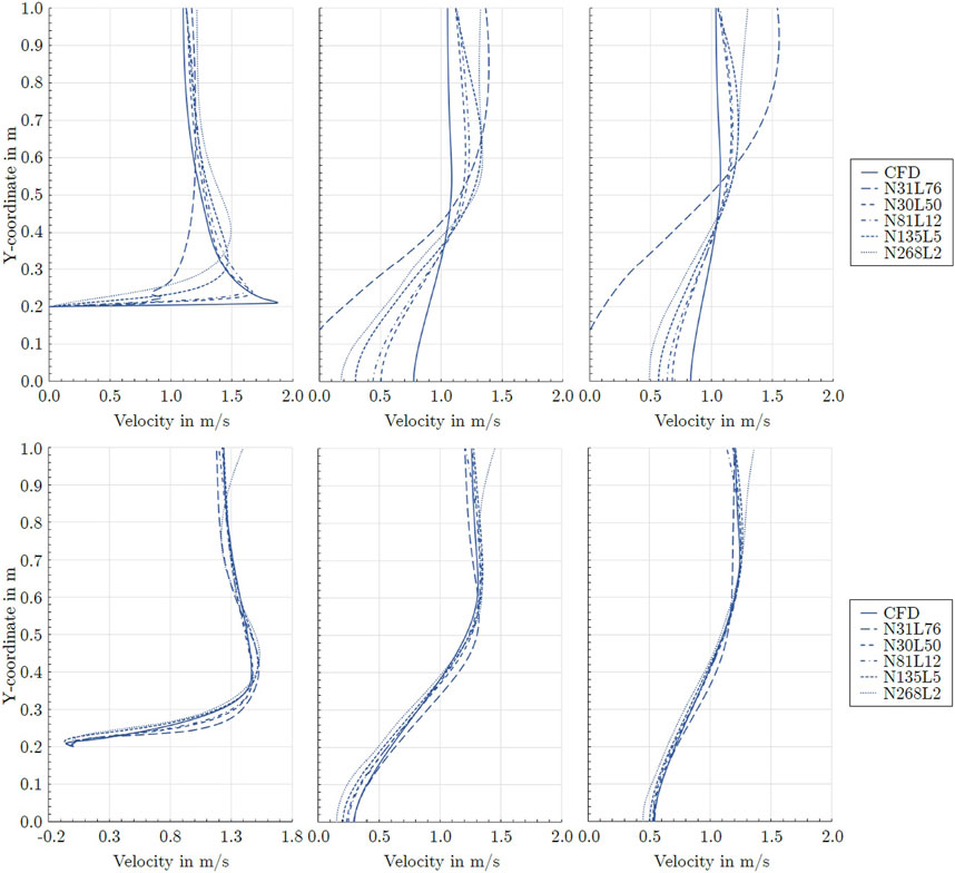
Figure 7. Axial velocities around the circular cylinder (top row) and the square cylinder (bottom row) at x = 0 m (left), x = 1 m (middle), and x = 2 m (right).

The trends observed for the axial velocity were also observed for the pressure field. Figures 8, 9 exhibit the pressure predictions and comparative CFD data. For the circular cylinder G1, model N31L76 predicted pressure values close to zero and did not capture the pressure field. For the square cylinder G2, model N31L76 predicted inaccurate results as well. Similarly, model N268L2 did not predict the pressure field accurately. For the circular cylinder, the positive pressure in the stagnation region of the reference solution was underestimated and a moderate negative pressure was predicted around the cylinder. For the square cylinder, model N268L2 predicted a dislocated region of positive pressure at the upstream side of the cylinder. For the circular cylinder, the best fitting model N50L30 captured the positive pressure region at the upwind side of the cylinder as well as the negative pressure at the lateral sides. However, the positive pressure on the downwind side was not predicted. For the square cylinder, the best fitting model N135L5 captured the positive pressure of the stagnation region as well as a negative pressure field around the square cylinder. However, size and magnitude of the positive pressure region as well as the negative pressure region at the upstream corners were underestimated.

Figure 8

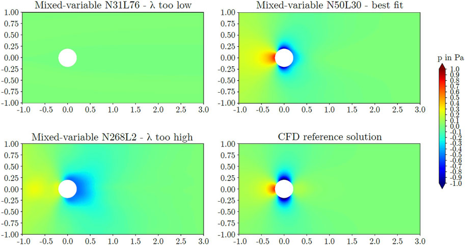
Figure 8. Predicted pressure around the circular cylinder obtained by the mixed-variable PINN method.

Figure 9

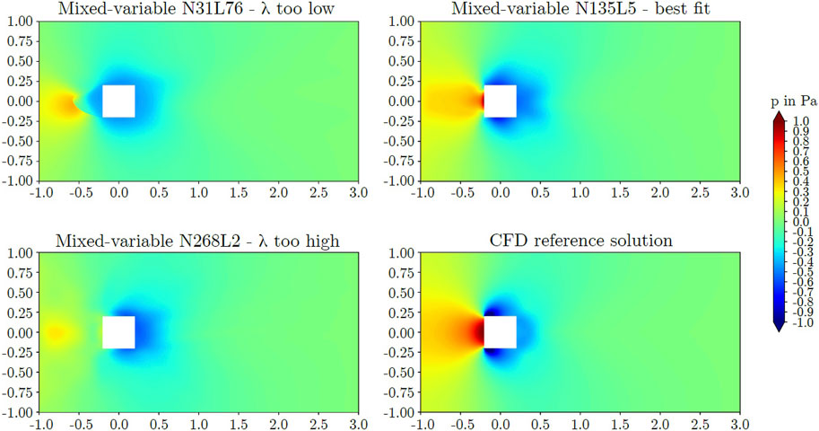
Figure 9. Predicted pressure around the square cylinder obtained by the mixed-variable PINN method.

The pressure values on the cylinder surface are shown in Figure 10. The deep but narrow model N31L76 predicted a vanishing pressure distribution around the entire cylinder. All models failed to predict the positive pressure region on the downstream side of the cylinder that was present in the CFD reference data. From all mixed-variable models, N50L30 provided the best representation of the reference solution. The minimum pressure peaks were more pronounced and the pressure on the downwind side of the cylinder was increased. Furthermore, the asymmetry associated with the other architectures was reduced. Figure 10 also exhibits a comparison between the pressure distributions on the square cylinder surface. Models N31L76 as well as N268L2 predicted inaccurate results. All other models captured the shift from positive to negative pressure. All networks underestimated the negative pressure maxima at the square edges that were featured by the CFD reference data. Models N50L30 and N81L12 better predicted the sharp shift from positive to negative pressure while model N135L5 more accurately matched the positive pressure magnitude at the upstream side of the square.

Figure 10

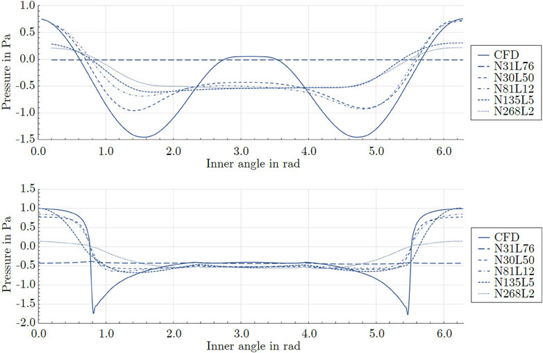
Figure 10. Pressure distributions on the circular cylinder (top) and the square cylinder (bottom).

For the circular cylinder G1, the best fitting PINN N50L30 predicted a drag of 0.272 N while the reference CFD yielded 0.135 N. The overestimation of the drag force correlated with an underestimation of the pressure in the wake at the downwind side of the cylinder when compared to the pressure distribution of the CFD reference solution. For the square cylinder, a drag force of 0.242 N was predicted by the best fitting model N135L5 while the reference solution featured a drag of 0.473 N. The underestimation of the drag correlated with an underestimation of the pressure values on the upwind side of the square.

The correlation of shape factor and mean squared error (MSE) is shown in Figure 11 for the circular cylinder G1. As seen, the axial velocity in the x-direction achieved the highest overall MSE. The relationship between MSE and shape factor was similar for all flow field variables. As λ tended to zero, the error increased markedly. For the networks with shape factors above 1.67 × 10⁰, the error grew with a decreasing slope. The obtained data suggests an optimal network shape for networks with shape factors close to 1.67 × 10⁰. For the best fitting model, N50L30, the losses for the two momentum equations were 9.23 × 10⁻⁶ and 6.99 × 10⁻⁶ for the x- and y-directions, respectively. The achieved losses indicate that the governing equations were satisfied. The correlation between MSE and shape factor was different for the two cylinder geometries. Figure 11 also displays the MSE of the different network shapes for the square cylinder G2. As seen, the error tended to a minimum for shape factors between 6.75 × 10⁰ and 2.70 × 10¹. For the square cylinder, the best shape factor was greater than for the circular cylinder. Furthermore, close to its minimum, the growth of the MSE was less and featured a broader region of minimal MSE. However, the models featuring the lowest NMSEs, i.e., N50L30 and N81L12 also featured artificial velocity peaks at the upstream corners of the square and, hence, were discarded. For model N135L5, featuring a shape factor of 2.70 × 10¹, the achieved losses for the momentum equations were 3.23 × 10⁻⁵ and 2.47 × 10⁻⁵. The minimal global MSEs for u, v, and p were lower for the square cylinder while the corresponding losses of the best model were lower for the circular cylinder.

Figure 11

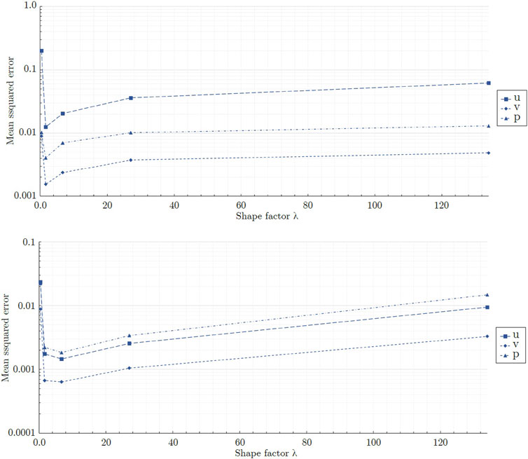
Figure 11. Global mean squared errors for the circular cylinder (top) and the square cylinder (bottom) obtained by the tested mixed-variable network architectures featuring progressing shape factors. For visualization purposes, the data points are connected by straight lines.

Figure 12 exhibits the MSEs obtained by the different network sizes featuring the best fitting shape factor 1.67 × 10⁰ for the circular cylinder. As seen, the network N20L12, featuring 4,780 trainable parameters, yielded the greatest errors. The corresponding predictions of the velocity field were inaccurate and comparable to that of model N268L2 shown in Figure 5. The other models, featuring a greater number of trainable parameters, yielded similar errors. Model N50L30, featuring 74,350 trainable parameters, was well within the size independent range and neither a reduction nor an increase of the number of trainable parameters led to a further reduction of the global MSE, indicating the superiority of this architecture. Figure 12 also exhibits the results of the evaluation of the network size for the square cylinder. In contrast to the circular cylinder, the global MSEs decreased over the entire range of tested network sizes. For model N54L2, featuring 3,402 trainable parameters, the highest errors were recorded, and the corresponding predictions were comparable to that of model N31L76 shown in Figure 6. Increasing the number of trainable parameters from 74,520 to 133,326 led to a reduction of 20%–30% of the global NMSE for model N162L6. However, the predictions showed no qualitative improvement and featured artificial velocity peaks at the upstream corners of the square. Hence, the larger model did not lead to more favorable predictions of the flow field.

Figure 12

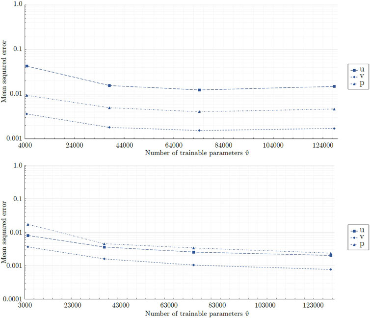
Figure 12. Global mean squared errors for on the circular cylinder (top) and the square cylinder (bottom) obtained by the mixed-variable network architectures featuring a constant shape factor of 2.70×10¹ and a progressing number of trainable parameters. For visualization purposes, the data points are connected by straight lines.

3.3 Validation of the mixed-variable method against measurements

Figure 13A) exhibits the axial velocity field for geometry G3 as predicted by model N81L12. As seen, the PINN captured a stagnation region of lower velocity at the upwind edge of the square as well as a wake at the downwind side of the cylinder. Furthermore, the high velocity areas extending from the upwind corners of the square were captured. Overall, the flow field was well captured. A comparison of the axial velocity as predicted by the PINN and the values obtained from the time averaged laser-Doppler measurements is shown in Figure 13B) for several vertical lines in the wake of the square cylinder. In the PINN predictions, the velocity deficit inside the wake was less pronounced at x/c = 1.0 and, due to momentum and mass conservation, a lower velocity was predicted at the outer extent of the shear layer at y/c = 1.0. Overall, there was a favorable agreement between the PINN predictions and the measured results, considering the small scale of the cylinder, the three-dimensional nature of the reference flow, and the absence of any simulated or measured data during training of the neural net.

Figure 13

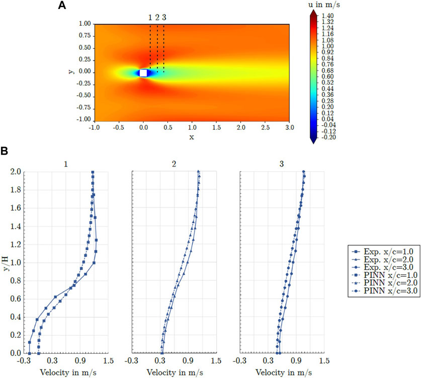
Figure 13. Predicted axial velocities compared with experimental results for geometry G3. (A) Contour plot of the predicted velocity obtained by the mixed-variable PINN; (B) Comparison with experimental data along several vertical lines in the wake of the square cylinder.

4 Discussion

The traditional PINNs failed to yield acceptable predictions for the elevated Reynolds number flow investigated here. For lower Reynolds number flows, successful training was reported by Ang et al. [1]. A major challenge of high Reynolds number flows is the increasing complexity of the optimization problem as the nonlinear convective momentum terms of the RANS equations become dominant, shear leayer gradients become steeper, and turbulence models increase the complexity of the RANS equations. Utilizing the mixed-variable approach advanced the training success of the PINN method. The success of the mixed-variable method can be attributed to the simplification of the complex optimization problem [26]. In contrast to the traditional method, no second-order derivatives of the velocities needed to be considered in the governing equations of the mixed-variable method. This was the crucial factor in attaining a more easily solvable optimization problem. The usage of the stream function further assisted the training by automatically enforcing the continuity equation. Nevertheless, accurate results can also be obtained without the usage of the stream variable. Due to the remaining complexity of the optimization problem, there were still deviations from the reference solution. This contrasts the excellent results of Rao et al. [26], obtained for a laminar low Reynolds number flow. Increasing errors associated with higher Reynolds numbers were also reported by Sun et al. [27] and Harmening et al. [6]. Consequently, numerous studies were conducted incorporating measured or simulated training data to support training of the PINN [3, 5, 8, 10, 19, 21, 35, 36], while investigations focusing unsupervised physics-informed DL of high Reynolds number flows without training data remain sparse [7].

The traditional models required significantly more computational time for training. The advantage of the mixed-variable method was between 90.6% and 161.2%, depending on the model. For the best fitting model N135L5, the traditional PINN method took 3.7 h which represents 105.5% more training time than necessary for the mixed-variable model. Besides, the two PINN methods featured comparable graphic memory requirements which were also depending on the network architecture. For model N135L5, 3.6 GB were consumed. For model N50L30, the mixed-variable model took 10.1 GB of graphic memory while the traditional model required 11.1 GB.

For the circular cylinder G1, the high gradients of the flow were not successfully learned by most network architectures. Only models N50L30 and N81L12 captured the boundary layer on the cylinder at x = 0. Furthermore, the wake length was predicted more accurately by model N50L30. For the square cylinder G2, models N135L5 and N81L12 exhibited superior performance. The flow separation and recirculation that was present on the lateral sides of the cylinder at x = 0 was best captured by model N135L5. However, model N81L12 achieved the lowest overall MSE. As the corresponding shape factors varied by up to one order of magnitude, distinct network architectures were necessary to capture the flow fields around the two geometries most accurately. These results imply that networks yielding accurate predictions in certain cases might significantly deviate from networks suitable for other cases. More work is needed to further investigate the best architectures for more complex geometries.

The superiority of the N50L30 architecture to predict the flow around the circular cylinder G1 as well as the square cylinder of geometry G3 agreed favorably with a study of Ang et al. [1], who identified a traditional PINN with 50 neurons per layer and a minimum of 20 hidden layers most suitable for a low Reynolds number flow around a circular cylinder. This corresponds to shape factors below 2.5 × 10⁰. Rao et al. [26] studied a laminar low Reynolds number flow and used a mixed-variable PINN comprising 40 neurons per hidden layer with a total of eight hidden layers. The network featured a shape factor of 5.0 × 10⁰ and comprised 15.9% of the trainable parameters contained in the N50L30 model used here. We investigated this architecture in preparation of our study as well; however, the model yielded unfavorable results similar to our models N268L2 or N20L12. Eivazi et. al [3] applied a network architecture of 20 neurons per layer and eight layers using the traditional PINN approach. The shape factor of this model was 2.5 × 10⁰ and featured 4.2% of the trainable parameters of the N50L30 model. Eivazi et. al reported good results for fractions of flow fields at elevated Reynolds numbers without using training data in the flow domain. However, for the flow we investigated, the architecture also exhibited unfavorable results similar to the high shape factor model N268L2 or the smaller model N20L12. As discussed above, network architectures and types that proved to be suitable for specific cases can not readily be applied to other cases and, consequently, a comprehensive screening of the best shape and size needs to be carried out.

The results revealed effects of the network shape as well as effects of the network size. The small models N20L12 and N54L2 yielded inferior results. An explanation is that the expressiveness was restricted by the limited number of the tuneable parameters. Consequently, the prediction accuracy increased with network size and the high gradients were captured more accurately. However, for the circular cylinder G1, the prediction accuracy stagnated for the large model N60L36, indicating an increasing relevance of other error sources. A different correlation was observed for the network shape and neither extremely deep nor extremely wide networks showed to be suitable. This suggests that a minimal depth was required to model the nonlinear high gradient solution field and the extremely deep and wide networks were less suitable due to an excessive complexity or limited representational capacity. However, a more precise explanation remains an open question due to the black box character of the neural network approach.

While preparing this study, methods including non-adaptive loss weighting for the traditional approach, hard boundary constraints [27], vorticity formulation of the RANS equations (9), Helmholtz decomposition [19], residual neural networks, and Fourier feature networks [32] were tested. However, these methods did not exhibit favorable results and, therefore, they are not discussed here in detail. Other turbulence models, such as an equation-free modeling approach [3, 21, 36], Prandtl’s one equation k model, and the k-ω model of Wilcox [33], were tested as well in preparation of this study. However, the traditional turbulence models suffered from stability issues during the training process, while the equation-free approach did not capture the flow field accurately. Applying the mixed-variable approach, considering the mixing length turbulence model in combination with networks featuring proper shape factors and sufficient trainable parameters, was the only method that was capable of capturing the stagnation points, high gradient boundary layers, and flow separation of the investigated high Reynolds number flow fields. Nevertheless, an extensive search for the best network shapes was necessary to obtain these results.

Yet, the effect of the shape factor and the network size on the prediction accuracy was limited. A remaining bias error regarding the wake length behind the circular cylinder, an overestimation of the stagnation region size for the square cylinder, as well as an underestimation of the pressure peaks on the cylinder surfaces was observed, documenting the difficulties associated with predicting high Reynolds number flows using PINNs. Hence, more work is needed to further increase the prediction accuracy of the mixed-variable method. The deviations between the mixed-variable predictions and the CFD reference solution were attributed to training or optimization errors, generalization errors, and approximation errors. Here, the approximation error is defined as the deviation between the target function or reference solution and the closest neural network function of a given architecture. The generalization error is a measure for the accuracy of the prediction for unseen data, here coordinates. The training or optimization error is then defined as the deviation between the closest network function attainable with the given set of training coordinates and the network function obtained after training under the given optimization algorithm settings. A modeling error concerning the RANS turbulence model also contributed to the differences between the PINN predictions and the measured velocities. As reported by Harmening et al. [6], the network and training related errors could be reduced to a minimum by introducing training data. Other potential methods to improve the accuracy include curriculum learning [12], adaptive loss weighting [15, 30, 32, 34], convolutional or U-Net PINNs [11, 18, 29, 31, 37], and distributed PINNs [2], among others. The geometries investigated here should serve as a benchmark case to evaluate such methods because the corresponding high Reynolds number flow fields feature a number of important flow phenomena that any reliable PINN methodology must be capable to capture.

The method investigated here may be used with and without labeled training data. As the mixed-variable approach yielded favorable results without using any training data, the required data quantities to train mixed-variable models agreeing with CFD or experimental studies can be expected to be minimal. The method may be used for improved interpolations and extrapolations between data points. The method without training data can be applied for comparative studies and optimization processes [7]. However, then the demonstrated limitations of the PINN models need be taken into account.

4.1 Summary and conclusion

We compared different network architectures using mixed-variable physics-informed deep learning and traditional PINNs with CFD and measured reference data. The models were trained to solve the two-dimensional RANS equations for a turbulent flow around a circular cylinder and a square cylinder. The mixing length turbulence model was deployed. The main findings are summarized as follows:

• For the elevated Reynolds number flow considered here, the superiority of the mixed-variable approach of Rao et al. [26] was confirmed. The traditional PINN method failed to capture the flow field accurately, independent of the network architecture.

• For the flow around the large scale circular cylinder, the deep architecture with a shape factor of 1.67 × 10⁰ outperformed the other architectures. The steep gradients of the boundary layers were predicted more accurately and the prolonged wake was reduced. For the flow around the large scale square cylinder, the wide network with a shape factor of 2.70 × 10¹ captured the reference solution best. The model with a shape factor of 6.75 × 10⁰ worked well for both geometries.

• For the geometries investigated, different mixed-variable network architectures with factors varying by one order of magnitude were suitable. This demonstrates that depending on the case, it might be necessary to distinctly vary the shape factor of a PINN to find the best fitting model. However, using extremely high or low shape factors proved to be inappropriate.

• Despite inevitable deviations from the reference flow fields, the physics-informed mixed-variable method applied with a proper network architecture was able to predict stagnation points, high gradient boundary layers, flow separation, recirculation areas, and wakes at an elevated Reynolds number without requiring training data. In contrast, regular neural nets are not capable to predict plausible flow fields without providing extensive training data inside the domain.

• The mixing length model proved to be a reliable and stable model for physics-informed deep learning when no simulated or measured data were considered.

• More work needs to be done concerning physics-informed deep learning of the RANS equations. Future work should consider other turbulence models and methods to further increase the accuracy of predicted high Reynolds number flows.

Data availability statement

The raw data supporting the conclusion of this article will be made available by the authors, without undue reservation.

Author contributions

JH: Conceptualization, Data curation, Investigation, Methodology, Project administration, Software, Validation, Visualization, Writing–original draft. F-JP: Resources, Supervision, Writing–review and editing. OM: Supervision, Writing–review and editing.

Funding

The author(s) declare that financial support was received for the research, authorship, and/or publication of this article. We acknowledge support by the Open Access Publication Fund of the Westphalian University.

Acknowledgments

We are grateful to Thomas Erling Schellin for review of the manuscript.

Conflict of interest

The authors declare that the research was conducted in the absence of any commercial or financial relationships that could be construed as a potential conflict of interest.

Publisher’s note

All claims expressed in this article are solely those of the authors and do not necessarily represent those of their affiliated organizations, or those of the publisher, the editors and the reviewers. Any product that may be evaluated in this article, or claim that may be made by its manufacturer, is not guaranteed or endorsed by the publisher.

References

1. Ang EHW, Wang G, Ng BF. Physics-informed neural networks for low Reynolds number flows over cylinder. Energies (2023) 16:4558. doi:10.3390/en16124558

CrossRef Full Text | Google Scholar

2. Dwivedi V, Parashar N, Srinivasan B. Distributed physics informed neural network for data-efficient solution to partial differential equations (2019). Preprint at http://arxiv.org/pdf/1907.08967v1.

Google Scholar

3. Eivazi H, Tahani M, Schlatter P, Vinuesa R. Physics-informed neural networks for solving Reynolds-averaged Navier–Stokes equations. Phys Fluids (2022) 34:075117. doi:10.1063/5.0095270

CrossRef Full Text | Google Scholar

4. European Research Community on Flow, Turbulence and Combustion (2023). Classic collection database: case043 (vortex shedding past square cylinder). [Online; Accessed 07.December.2023]

Google Scholar

5. Ghosh S, Chakraborty A, Brikis GO, Dey B. Rans-pinn based simulation surrogates for predicting turbulent flows (2023). Preprint at https://arxiv.org/pdf/2306.06034.pdf.

Google Scholar

6. Harmening JH, Pioch F, Fuhrig L, Peitzmann F-J, Schramm D. Data-assisted training of a physics-informed neural network to predict the Reynolds-averaged turbulent flow field around a stalled airfoil under variable angles of attack (2023). Preprint at https://www.preprints.org/manuscript/202304.1244/v1.

Google Scholar

7. Hennigh O, Narasimhan S, Nabian MA, Subramaniam A, Tangsali K, Fang Z, et al. Nvidia simnet^TM: an ai-accelerated multi-physics simulation framework. Lecture Notes Comput Sci (2021) 12746:447–61. doi:10.1007/978-3-030-77977-1_36

CrossRef Full Text | Google Scholar

8. Huang W, Zhang X, Zhou W, Liu Y. Learning time-averaged turbulent flow field of jet in crossflow from limited observations using physics-informed neural networks. Phys Fluids (2023) 35. doi:10.1063/5.0137684

CrossRef Full Text | Google Scholar

9. Jin X, Cai S, Li H, Karniadakis GE. Nsfnets (Navier-Stokes flow nets): physics-informed neural networks for the incompressible Navier-Stokes equations. J Comput Phys (2021) 426:109951. doi:10.1016/j.jcp.2020.109951

CrossRef Full Text | Google Scholar

10. Kag V, Seshasayanan K, Gopinath V. Physics-informed data based neural networks for two-dimensional turbulence. Phys Fluids (2022) 34. doi:10.1063/5.0090050

CrossRef Full Text | Google Scholar

11. Kim Y, Choi Y, Widemann D, Zohdi T. A fast and accurate physics-informed neural network reduced order model with shallow masked autoencoder. J Comput Phys (2022) 451:110841. doi:10.1016/j.jcp.2021.110841

CrossRef Full Text | Google Scholar

12. Krishnapriyan A, Gholami A, Zhe S, Kirby R, Mahoney MW. Characterizing possible failure modes in physics-informed neural networks. In: M Ranzato, A Beygelzimer, Y Dauphin, PS Liang, and J Wortman Vaughan, editors. Advances in neural information processing systems, 34. Curran Associates, Inc (2021). p. 26548–60.

Google Scholar

13. Lagaris IE, Likas A, Fotiadis DI. Artificial neural networks for solving ordinary and partial differential equations. IEEE Trans Neural networks (1998) 9:987–1000. doi:10.1109/72.712178

PubMed Abstract | CrossRef Full Text | Google Scholar

14. Laubscher R, Rousseau P. Application of a mixed variable physics-informed neural network to solve the incompressible steady-state and transient mass, momentum, and energy conservation equations for flow over in-line heated tubes. Appl Soft Comput (2022) 114:108050. doi:10.1016/j.asoc.2021.108050

CrossRef Full Text | Google Scholar

15. Li S, Feng X. Dynamic weight strategy of physics-informed neural networks for the 2d Navier-Stokes equations. Entropy (2022) 24:1254. doi:10.3390/e24091254

PubMed Abstract | CrossRef Full Text | Google Scholar

16. Lu L, Meng X, Mao Z, Karniadakis GE. Deepxde: a deep learning library for solving differential equations. SIAM Rev (2021) 63:208–28. doi:10.1137/19M1274067

CrossRef Full Text | Google Scholar

17. Lyn DA, Einav S, Rodi W, Park J-H. A laser-Doppler velocimetry study of ensemble-averaged characteristics of the turbulent near wake of a square cylinder. J Fluid Mech (1995) 304:285–319. doi:10.1017/S0022112095004435

CrossRef Full Text | Google Scholar

18. Ma H, Zhang Y, Thuerey N, null XH, Haidn OJ. Physics-driven learning of the steady Navier-Stokes equations using deep convolutional neural networks. Commun Comput Phys (2022) 32:715–36. doi:10.4208/cicp.OA-2021-0146

CrossRef Full Text | Google Scholar

19. Patel Y, Mons V, Marquet O, Rigas G. Turbulence model augmented physics informed neural networks for mean flow reconstruction (2023). Preprint at http://arxiv.org/pdf/2306.01065v1.

Google Scholar

20. Pinkus A. Approximation theory of the mlp model in neural networks. Acta Numerica (1999) 8:143–95. doi:10.1017/S0962492900002919

CrossRef Full Text | Google Scholar

21. Pioch F, Harmening JH, Müller AM, Peitzmann F-J, Schramm D, el Moctar O. Turbulence modeling for physics-informed neural networks: comparison of different rans models for the backward-facing step flow. Fluids (2023) 8:43. doi:10.3390/fluids8020043

CrossRef Full Text | Google Scholar

22. Raissi M, Perdikaris P, Karniadakis GE. Physics informed deep learning (part i): data-driven solutions of nonlinear partial differential equations (2017). Preprint at http://arxiv.org/pdf/1711.10561v1.

Google Scholar

23. Raissi M, Perdikaris P, Karniadakis GE. Physics informed deep learning (part ii): data-driven discovery of nonlinear partial differential equations (2017). Preprint at http://arxiv.org/pdf/1711.10566v1.

Google Scholar

24. Raissi M, Perdikaris P, Karniadakis GE. Physics-informed neural networks: a deep learning framework for solving forward and inverse problems involving nonlinear partial differential equations. J Comput Phys (2019) 378:686–707. doi:10.1016/j.jcp.2018.10.045

CrossRef Full Text | Google Scholar

25. Raissi M, Yazdani A, Karniadakis GE. Hidden fluid mechanics: learning velocity and pressure fields from flow visualizations. Science (New York, N.Y.) (2020) 367:1026–30. doi:10.1126/science.aaw4741

PubMed Abstract | CrossRef Full Text | Google Scholar

26. Rao C, Sun H, Liu Y. Physics-informed deep learning for incompressible laminar flows. Theor Appl Mech Lett (2020) 10:207–12. doi:10.1016/j.taml.2020.01.039

CrossRef Full Text | Google Scholar

27. Sun L, Gao H, Pan S, Wang J-X. Surrogate modeling for fluid flows based on physics-constrained deep learning without simulation data. Comput Methods Appl Mech Eng (2020) 361:112732. doi:10.1016/j.cma.2019.112732

CrossRef Full Text | Google Scholar

28. Thuerey N, Weißenow K, Prantl L, Hu X. Deep learning methods for Reynolds-averaged Navier–Stokes simulations of airfoil flows. AIAA J (2020) 58:25–36. doi:10.2514/1.J058291

CrossRef Full Text | Google Scholar

29. Wandel N, Weinmann M, Klein R. Teaching the incompressible Navier–Stokes equations to fast neural surrogate models in three dimensions. Phys Fluids (2021) 33:047117. doi:10.1063/5.0047428

CrossRef Full Text | Google Scholar

30. Wang H, Liu Y, Wang S. Dense velocity reconstruction from particle image velocimetry/particle tracking velocimetry using a physics-informed neural network. Phys Fluids (2022) 34:017116. doi:10.1063/5.0078143

CrossRef Full Text | Google Scholar

31. Wang R, Kashinath K, Mustafa M, Albert A, Yu R. Towards physics-informed deep learning for turbulent flow prediction. In: R Gupta, Y Liu, M Shah, S Rajan, J Tang, and BA Prakash, editors. Proceedings of the 26th ACM SIGKDD international conference on knowledge discovery and data mining. New York, NY, USA: ACM (2020). p. 1457–66. doi:10.1145/3394486.3403198

CrossRef Full Text | Google Scholar

32. Wang S, Sankaran S, Wang H, Perdikaris P. An expert’s guide to training physics-informed neural networks (2023). Preprint at https://arxiv.org/pdf/2308.08468.pdf.

Google Scholar

33. Wilcox DC. Reassessment of the scale-determining equation for advanced turbulence models. AIAA J (1988) 26:1299–310. doi:10.2514/3.10041

CrossRef Full Text | Google Scholar

34. Xiang Z, Peng W, Liu X, Yao W. Self-adaptive loss balanced physics-informed neural networks. Neurocomputing (2022) 496:11–34. doi:10.1016/j.neucom.2022.05.015

CrossRef Full Text | Google Scholar

35. Xiao M-J, Yu T-C, Zhang Y-S, Yong H. Physics-informed neural networks for the Reynolds-averaged Navier–Stokes modeling of Rayleigh–taylor turbulent mixing. Comput Fluids (2023) 266:106025. doi:10.1016/j.compfluid.2023.106025

CrossRef Full Text | Google Scholar

36. Xu H, Zhang W, Wang Y. Explore missing flow dynamics by physics-informed deep learning: the parameterized governing systems. Phys Fluids (2021) 33:095116. doi:10.1063/5.0062377

CrossRef Full Text | Google Scholar

37. Zhu Y, Zabaras N, Koutsourelakis P-S, Perdikaris P. Physics-constrained deep learning for high-dimensional surrogate modeling and uncertainty quantification without labeled data. J Comput Phys (2019) 394:56–81. doi:10.1016/j.jcp.2019.05.024

CrossRef Full Text | Google Scholar