Potential of N-CovSel for Variable Selection: A Case Study on Time-Series of Multispectral Images

1 Introduction

From the point of view of data visualisation and interpretation, multi-way analysis allows simplification of the results, providing more adequate and robust models using relatively few parameters (Salvatore et al., 2013). According to Henrion (1994), as information becomes more complex, i.e., extremely diverse in terms of information, size and behaviour, the concept of a “data set” naturally expands from traditional tables, such as matrices, to higher-dimensional arrays. In fact, the use of multi-way analysis allows connected pieces of information to reflect variation spread across components, events or sources that are represented differently and, yet, complement each other in the simultaneously analysed data (de Juan and Tauler, 2019). Multispectral imaging (MSI) is a well-known imaging techniques that has its origins in remote sensing. In practice, regardless of the applications, different approaches to deal with the increasing data volumes and variability of the data from satellite based time-series imaging, such as Sentinel-2 (A/B), can be found in the remote sensing literature (Picoli et al., 2020). In recent years, spatial-spectral feature extraction has been a developing field of research managing high-dimensional data (Hong et al., 2020). However, in addition to spatial information, the Sentinel-2 satellites contain spectral information with 5-day revisit time, which provides a detailed overview of land and vegetation.

Multispectral imaging techniques applied to temporal series represent an important research tool to assess the impacts of Climate Change (CC) on agricultural systems as it allows spatially and temporally continuous phenomenon to be monitored. The main abiotic factors in the life cycle of crops, especially during the growing period, are weather conditions, which determine the quantity and quality of agricultural production (Raza et al., 2019). One of the most measurable effects of CC is the gradual rise in temperature, which leads to an increase in the frequency and severity of extreme weather events (Droulia and Charalampopoulos, 2021). According to Venios et al. (2020) fluctuations in environmental conditions, particularly ambient temperature, strongly influence plant growth and development processes. As a result, remote sensing has the potential ability to assess the impact of an extreme weather effect, e.g., a heatwave, as the reflectance spectrum changes depending on growth circumstances and the time of measurement relative to the stage of crop development (Filella et al., 1995; Cogato et al., 2019). However due to the complexity of combining spatial, spectral, and temporal information derived from remote sensing, there are still challenges in dealing with increased data volumes and variability of these data (Bishop, 2013). Making the most of multispectral image time-series is a promising but still relatively underexplored research direction in the context of life sciences.

The use of multi-way analysis in remote sensing, such as N-way partial least squares (N-PLS) regression, shares all the advantages of latent-based regression and discrimination methods, i.e., data visualisation and interpretation (Favilla et al., 2013; Lopez-Fornieles et al., 2022). In addition, it allows the representation of data patterns, feature correlation and covariance structure characteristic over time-series images (Coppi, 1994; Favilla et al., 2013). When a two-dimensional signal characterizes each sample, as generated by MSI, such as wavelength/time information, it is often needed to define which are the most relevant features to predict the studied dependent properties. When it comes to deal with complex datasets, a generalised option is the selection of variables (or feature extraction) (Trevino and Falciani, 2006) as these methods allow to: 1) select relatively small number of total variables and restrict it to the most significant ones, i.e., for subsequent application in regression/classification models and 2) to understand which variable contributes the most to the investigated system, i.e., interpretative purposes (Biancolillo et al., 2021). Several variable selection methodologies have been proposed in the literature (Mehmood et al., 2012), and yet most of variable selection methods refer to contexts in which data is collected in a matrix rather than a in higher-order structure, thus loosing the multi-way analysis advantage (Favilla et al., 2013). However, Biancolillo et al. (2022) proposed an alternative variable selection approach for multi-way data, N-way Covariance Selection (N-CovSel). The N-CovSel algorithm is based on the same main principle as the covariance selection algorithm (CovSel) introduced by Roger et al. (2011) for data collected in data matrices. The latter approach is designed to select variables in regression and discrimination contexts, and to assess the relevance of variables based on their covariance with the response(s). Iteratively, the predictor with the highest covariance is selected and the data matrix (X) and the variable of interest to predict (y) are orthogonalised with respect to this variable (Biancolillo et al., 2022). By providing filter selection based on model parameters and integrating them into the model construction, the N-CovSel algorithm opens the possibility to select information in a complex dataset as a multi-directional structure.

Regarding agricultural systems and CC impact with time-series of multispectral images, such a variable selection approach for high order data arrays, could bring a better understanding of how crop growth dynamic is affected by the occurrence of an extreme weather event. Therefore, the objectives of this study are to 1) propose a formalism to apply the N-CovSel approach to a time-series of images at the regional scale in order to predict a small variable of interest, 2) to show the value of methods originally developed in the analytical chemistry domain to be applied to larger scales and life sciences domains and 3) to identify the possible limitations of the approach when dealing with time series of satellite images.

The work is organized as follows: Section 2 introduces the proposed N-CovSel algorithm and the development of the model as well as the description of the case study that the methodology is applied to. The results are showed in Section 3, with the discussion in Section 4.

2 Materials and Methods

2.1 Notations

Upper case bold and underlined characters will be used for N-way arrays, e.g., X (I,J,K) indicates a 3-way array with I samples described by J times at K wavelengths. Upper case bold characters will be used for matrices, e.g., X and lower case bold characters will be used for column vectors, e.g., y. Non-bold italics will be used for scalars. Upper case characters for fixed values, e.g., the number of samples I and lower case characters will be used for running indexes, e.g., a slice k from the third mode of X. A column of X will be noted x_{. jk} and a slice of X will be noted X_{. j.} or X_{. k..}

The N-CovSel method allows the selection of the best set of predictors (features) in an N-way array (X) on the basis of its covariance with a response vector (y) or a response matrix (Y) (Biancolillo et al., 2022).

2.1.1 Definition of Features

When selecting features in a N-way array, different solutions are possible. In fact, it is possible to define different features depending on the number of way arrays of the input data structure. As determined by Biancolillo et al. (2022), for a 3-way data, i.e., a cube, two distinct options are possible: 1) a 2-D feature (Figures 1A,B), i.e., a variable in one mode without discarding any variable in the other (e.g., a slice ${\mathrm{X}}_j$ or a slice ${\mathrm{X}}_k$) and 2) a 1-D feature (Figure 1C), i.e., a single variable in each mode, e.g., the column $\left({\mathrm{x}}_{jk}\right)$.

FIGURE 1

FIGURE 1. Features in a 3-way array represented in (A) J-axis slice, (B) K-axis slice and (C) J,K-column (Biancolillo et al., 2022).

2.1.2 Algorithm

N-CovSel algorithm is an extension of the above mentioned CovSel feature selection approach by Roger et al. (2011) to high-order data. To assess the relevance of features in a 3-way array (X) context to predict a response vector y relying on covariance, Biancolillo et al. (2022) defined the N-CovSel algorithm as follows:

1) Determine the structure of the features to be selected, i.e., columns or slices.

2) Define the number of features to be selected.

3) Select the feature of X with the highest squared covariance with y.

4) Deflate X of the information present in the selected feature.

5) Continue from Step 3 until the value defined in step 2 is reached.

2.2 Case-Study

The Languedoc-Roussillon (LR) wine-growing area experienced a heatwave from the 23rd of June to the 8th July of 2019, with temperatures reaching 45°C on 28th June 2019. Extreme weather events, such as a heatwave, occurring on very rapid time scales during crucial periods of vine plant development (e.g., growing stage) will induce symptoms that may lead to stalled development, leaf burn and leaf drop (Schymanski et al., 2013; Lopez-Fornieles et al., 2022). According to Cogato et al., 2019, remote sensing data could provide valuable information from spectral-temporal dimensions to characterise the impact of heatwaves on perennial crops by providing a detailed time series of data on the physiological and physical properties changes of the cultivation (Plant et al., 2000).

The N-CovSel algorithm should therefore constitute a relevant approach to create a model on a reduced set of information highlighting the extreme weather phenomenon taking into account its spectral-temporal evolution.

2.2.1 Ground Truth Data

Ground truth data were selected from 107 non-irrigated vineyard blocks in the northern part of the LR region that all showed some effects related to the heatwave (Figure 2A). The severity of this effect was assessed by winegrowers and advisors on each of the 107 vineyard blocks by estimating the percentage of yield loss several weeks after 28th June 2019 corresponding to the peak of the extreme weather event. Severity was assessed several weeks later by estimating the percentage yield loss based on heat wave-related effects such as stalled development, scorching and leaf drop. It was acknowledged that it was sometimes difficult to attribute losses exclusively to the heatwave. Figure 2B summarises the distribution of the 107 blocks according to yield loss.

FIGURE 2

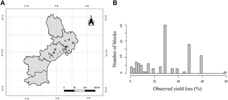
FIGURE 2. (A) Map of the 107 ground truthed blocks with known estimated percentage of yield loss after the heatwave and (B), percentage of yield losses observed by winegrowers and advisors on 107 vine blocks in southern France (Lopez-Fornieles et al., 2022).

2.2.2 Remote Sensing Data

Satellite images were selected via the Google Earth Engine (GEE) platform that provides Sentinel-2 L2A products. Sentinel-2 (A/B) satellites, with a revisit frequency of 10 days (5 days with the twin satellites together), provide 13 spectral bands from visible (Vis) to shortwave infrared (SWIR) with a spatial resolution of 10, 20 and 60 m depending on the spectral band (Table 1) (Lopez-Fornieles et al., 2022). Spectral band 10at 1,380 nm was not used in this study as it is designed for the detection of visible and sub-visible cirrus clouds (Hollstein et al., 2016).

TABLE 1

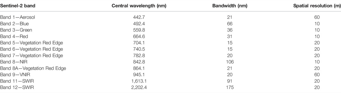
TABLE 1. Spectral bands for the Sentinel-2 satellite considered by the analysis.

Images containing the study vineyards (Section 2.3.1) were selected and processed via Google Earth Engine (GEE) (Lopez-Fornieles et al., 2022). Images were selected over a period encompassing the heatwave event; from 13th May to the 20th August 2019. Before calculating the average pixel values for each block, each date and each waveband, in order to avoid mixed pixels: 1) blocks boundary were extracted from the graphical parcel register of France (RPG) and 2) a 10 m inner-buffer was imposed over the boundary of each block (Lopez-Fornieles et al., 2022).

For the time period considered for the study (from May to August), defined as the most relevant period for monitoring vine growth vegetation in LR region (Devaux et al., 2019), 25 images should have been potentially available on each block. However, the number of images per block varied according to the local atmospheric conditions over each block for each acquisition date (Lopez-Fornieles et al., 2022). The number of available images for each block was 11 on average, being eight the standard deviation of the set of values.

2.2.3 Modelling

2.2.3.1 Data Array Construction

To overcome the challenge of heterogeneity in the number of images per block, an interpolation was performed to obtain a continuous data cube X (I × J × K). The interpolation at a date t was done wavelength by wavelength, by a convolution of the chronology measured with a Gaussian filter (Alam et al., 2008) in order to have a consistent time step dimension (J) between the 13th May and 20th August 2019. The parameters involved in the interpolation setting were fixed to the Gaussian filter width (P) = 30 and date interval (N) = 5.

At the end of the interpolation step, the data set was meaningfully arranged in a three-way array X of dimensionality 107 (samples, I) × 19 (times, J) × 12 (wavelengths, K) and a vector y (107), corresponding to the yield loss rates of the 107 blocks.

2.2.3.2 Model Calibration and Validation

A calibration and validation subset were created to build and evaluate the model. Considering the samples from the variable to be predicted, a calibration set (3/4) and a test set (1/4) have been defined by its distribution (Figure 2B), as follows Lopez-Fornieles et al. (2022):

1) The vector y was sorted in ascending order.

2) After sorting, every fourth individual was placed in the validation set and the others were kept in the calibration set.

At the end of this step, the data were therefore: 1) a calibration set X_c (I = 80, J = 19, K = 12) and 2) a test set X_t (I = 27, J = 19, K = 12).

2.2.3.3 Regression Model Application

As explained in Section 2.1, when selecting features in a 3-way array, different outcomes of N-CovSel were obtained. Thus, the structure of the initial data was reduced in either time or wavelengths slices (2-D features) or in columns (1-D features), i.e., date-wavelength coupling.

For the structure features (F) in 2-D, the number of best features in the calibration set was defined as follows:

1) For the temporal slices (Figure 1A), the number of features defined was F = 15. Thus the F = 15 dates were sorted in decreasing order of interest, providing a list of indices {j₁, j₂, …, j_F}.

2) For the spectral slices (Figure 1B), as the total number of Sentinel-2 satellites wavelengths is 12, the number of features defined was F = 12. Thus, the F = 12 wavelengths were sorted in decreasing order of interest, providing a list of indices {k₁, k₂, …, k_F}.

3) For the structure features in 1-D (Figure 1C), the number features defined was F = 15. Thus, the F = 15 date-wavelength coupling were sorted in decreasing order of interest, providing a list of pairs of indices {(j₁,k₁), (j₂,k₂), …, (j_F,k_F)}.

Once the N-CovSel algorithm had selected the variables’ relevancy on the basis of their covariance with the response(s) (Biancolillo et al., 2022), a regression model adapted to the reduced data set was applied. Depending on the structure of the selected features, different data analysis strategies can be applied. In the case of 2-D, as the feature selection is of higher order, features have been analysed using multi-way approach, whereas in the case of 1-D the most intuitive option was combine them into a matrix, and then applying a traditional chemometric approach (Biancolillo et al., 2022), as follows:

1) For the temporal slices, F = 15 N-way Partial Least Squares (N-PLS) models (Bro, 1996) were then calculated on the calibration set, using the slices {j₁}, {j₁, j₂}, …, {j₁, j₂, …, j_F}.

2) For the spectral slices, F = 12 N- PLS models (Bro, 1996) were then calculated on the calibration set, using the slices {k₁}, {k₁, k₂}, …, {k₁, k₂, …, k_F}.

3) For the columns (date-wavelength), F = 15 Partial Least Squares (PLS) models (Wold et al., 2001) were then calculated on the calibration set, using the columns {(j₁,k₁)}, {(j₁,k₁), (j₂,k₂)}, …, {(j₁,k₁), (j₂,k₂),…, (j_F,k_F)}.

Figure 3 summarises the workflow of the N-CovSel model calibration, and its implementation for a regression model according to the structure of its outcomes (slice or column).

FIGURE 3

FIGURE 3. Workflow diagram of the N-CovSel model calibration and the suitable choice of the regression method according to the structure of the features selected by the algorithm.

2.2.3.4 Model Evaluation

For each regression model calculated (N-PLS and PLS), a Standard Error of Calibration (SEC) was calculated, using the maximum number of latent variables (LV). In addition, a cross-validation of eight random blocks repeated 20 times, provided a Standard Error of Cross-Validation (SECV), using the same number of LVs. The joint analysis of SEC and SECV, according to the specific features (F) of the models, either according of the number of slices used (2-D) or the number of date-wavelength couplings used (1-D) was considered for the selection of optimal N-PLS and PLS models, respectively.

These three different PLS models (two multi-way and one uni-way) were then applied to the test set. Bias and Standard Error of Prediction (SEP) were calculated on this prediction. Thus, the predictive performance of the regression models was quantified by the square of the correlation coefficient r², the bias and the standard error parameters in the calibration and test subsets.

3 Results

3.1 Three-Way Data Array Over the Study Case

The remote sensing data were organised in a three-way array (X) without temporal data gaps due to clouds and inconsistent number of available satellite images. Figure 4 shows the interpolated spectra on the J = 19 dates, for the I = 107 plots (Section 2.3.3).

FIGURE 4

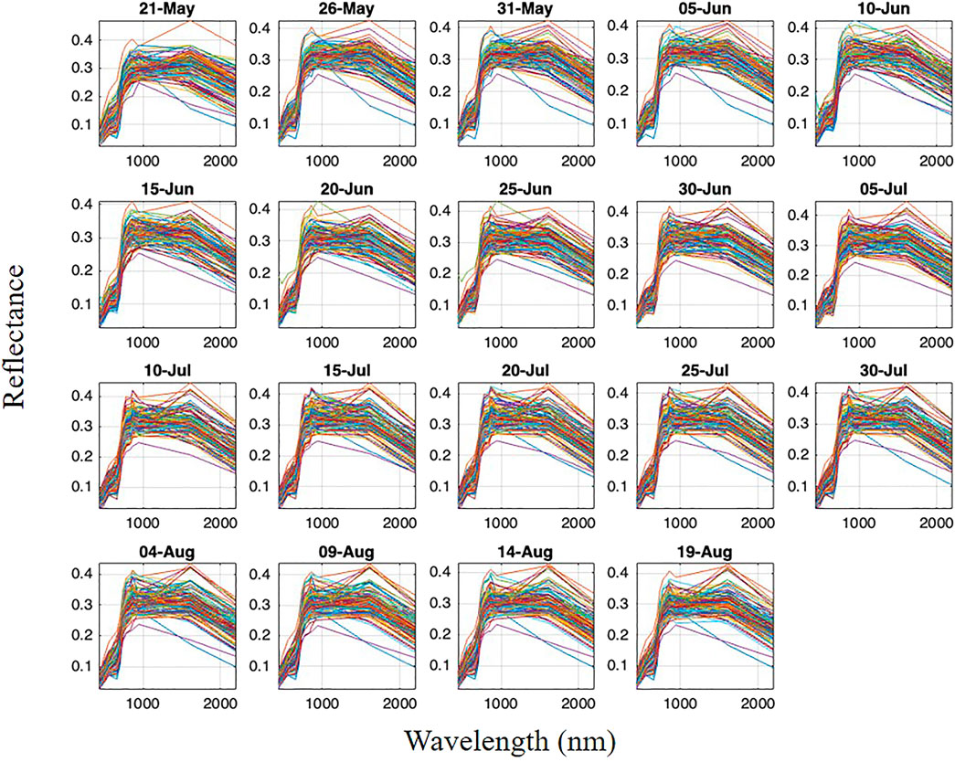
FIGURE 4. Interpolated spectra on the J = 19 dates, for the I = 107 plots.

Figure 4 shows typical properties of a time series that should not be neglected in satellite-based studies and applications. A high correlation between wavelengths was observed for nearby dates, which can be explained by the following factors: 1) remote sensing data sets themselves tend to be data structures with high covariance and redundancy (Lopez-Fornieles et al., 2022) and, 2) by interpolating missing data, the correlation within the multivariate data structure was increased. Moreover, other potential sources of uncertainties such as multiplicative and additive effects may have affected the reflectance measurement values for the interpolated spectra (Richter et al., 2012). According to Liu et al. (2006), the combination of factors such as varying atmospheric conditions, varying sun-target-satellite geometry and sensor degradation could influence the final measurement value on time-series images by causing the above-mentioned effects.

3.2 Quality of the Regression Models

Figure 5 shows the evolution of the SEC and SECV of an N-PLS for a cross-validation of eight blocks repeated 20 times of a N-PLS calibrated on the temporal (Figure 5A) and the spectral (Figure 5B) slices selected by N-CovSel algorithm. It should be noted that the selected features, either dates or wavelengths, were ordered by the N-CovSel algorithm from highest to lowest covariance between the calibration set (X_c) and the y-vector (ground truth data).

FIGURE 5

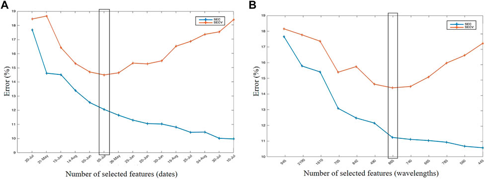
FIGURE 5. Evolution of the SEC and the SECV criteria for an 8-block, 20-fold cross-validation of a N-PLS between (A) the temporal features (slices) selected by N-CovSel and the y losses and (B) the spectral features (slices) selected by N-CovSel and the y losses. The black frame indicates the optimal number of (A) temporal features (F = 6) and (B) spectral features (F = 7) selected.

This figure highlights a classical phenomenon for both graphs: a phase of decrease of the SEC, which corresponds to an improvement of the explanatory value of features, then a phase of increase of the SECV (while the SEC keeps on decreasing), which corresponded to the overlearning phase. On the basis of this joint analysis, the appropriate number of features for the two different N-PLS models were six temporal slices (Figure 5A) and seven spectral slices (Figure 5B).

Figure 6 presents the evolution of the SEC and SECV criteria for a cross-validation of eight blocks repeated 20 times of a PLS calibrated on the date-wavelength columns selected and sorted by N-CovSel algorithm. On the basis of this joint analysis, the suitable number of features for the PLS model were nine date-wavelength columns.

FIGURE 6

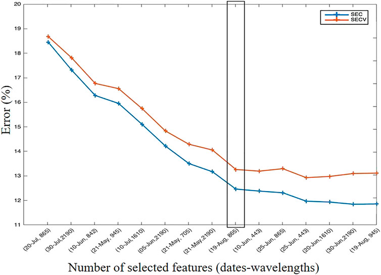
FIGURE 6. Evolution of the SEC and the SECV criteria for an 8-block, 20-fold cross-validation of a PLS between the date-wavelength features (columns) selected by N-CovSel algorithm and the y losses. The black frame indicates the optimal number of columns (F = 9) selected.

The quality and performance of the temporal and spectral N-PLS models and of the date-wavelength-pair PLS model are presented in terms of the standard error of calibration (SEC), the standard error of cross-validation (SECV) in the calibration set, the standard error of prediction of losses (SEP) in the test set, r² and the bias (Table 2).

TABLE 2

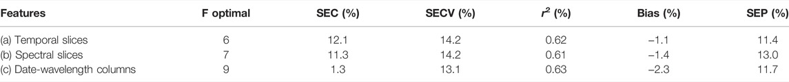
TABLE 2. (a) N-PLS yield loss prediction results using the first six slices (temporal) selected by N-CovSel algorithm on individuals in the calibration set, with 80 vineyard blocks and in the test set, with 27 vineyard blocks. (b) N-PLS yield loss prediction results using the first seven slices (spectral) selected by N-CovSel algorithm on individuals in the calibration set, with 80 vineyard blocks and in the test set, with 21 vineyard blocks. (c) PLS yield loss prediction results using the first nine pairs (date-wavelegth) selected by N-CovSel algorithm on individuals in the calibration set, with 80 vineyard blocks and in the test set, with 27 vineyard blocks.

A SEP over the predictions set between 11 and 13% (Table 2) was consistent with the initial variability of the ground truth data (Section 2.3.1) due to the information required by the winegrowers to correctly characterise the level of the heatwave impact on a vineyard block.

3.3 Interpretation of the selected features

3.3.1 Extraction of 2-D Features

3.3.3.1 Temporal Slices

Figure 7 illustrates the operation of the N-CovSel algorithm, searching for 2-D features along temporal mode. Each sub-figure corresponds to the selection of a 2-D feature, i.e., a date. Each subplot represents $co{v}^2({\mathrm{X}}_j,\mathrm{y})$ as a function of the temporal dimension; the maximum of each curve corresponds to the selected features of X in the second dimension with the highest squared covariance with y.

FIGURE 7

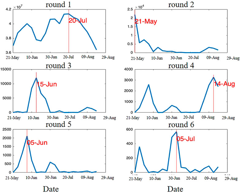
FIGURE 7. Evolution curves of ${\mathrm{cov}}^2\left({\mathrm{X}}_j,\mathrm{y}\right)$ as the first six temporal slices were selected by N-CovSel. The selected feature corresponds to the maximum of each curve; the corresponding dates are shown in red.

Each subplot (round) shows clear peaks, allowing the identification of dates involved in the prediction of yield losses. It should be noted that, for each round, the algorithm highlighted a different date of the time-series. Indeed, each curve showed a low value area around the previously selected variable and the overall amplitude of the curves for each round decreased as the features were extracted. These two particularities ensured that the selected features were at most complementary, i.e., at least correlated.

The first round showed three local peaks (5th June, 30th June and 20th July) which did not appear in the subsequent rounds until the fifth one (5th June), meaning that the peaks, as well as their information, were correlated with each other. Thus, the information retained for the 20th (the global maximum peak) of July translated the information of a continuous spectral phenomenon from the beginning of June to the end of July that conditioned the final yield losses of the vineyard blocks, i.e., round one showed a phenomenon independent of heat stress. The second round represented the first available date of the study period and the third round (15th June) highlighted a date prior to heat stress. This indicated that the initial conditions of the vineyard blocks (before the extreme weather event) were also related to the observed final yield losses. The sixth round was the most indicative of the heatwave that occurred between 23rd June and 8th July 2019 in view of their time frame. The fourth round showed two local peaks, on 14th August and 5th June and the fifth round showed the global peak on one same date, the 5th of June. This implied that as these were two consecutive rounds, the information contained in the 14th August (round 4) was independent from the 5th June round (round 5) in terms of final yield losses, i.e., the two dates were not correlated.

3.3.3.2 Spectral Slices

Figure 8 illustrates the operation of the N-CovSel algorithm, searching for 2-D features along spectral mode. Each sub-plot corresponds to the selection of a 2-D feature, i.e., a wavelength. Each subplot represents $co{v}^2\left({\mathrm{X}}_k,\mathrm{y}\right)$ as a function of the spectral dimension; the maximum of each curve corresponds to the selected features of X in the third dimension with the highest squared covariance with y.

FIGURE 8

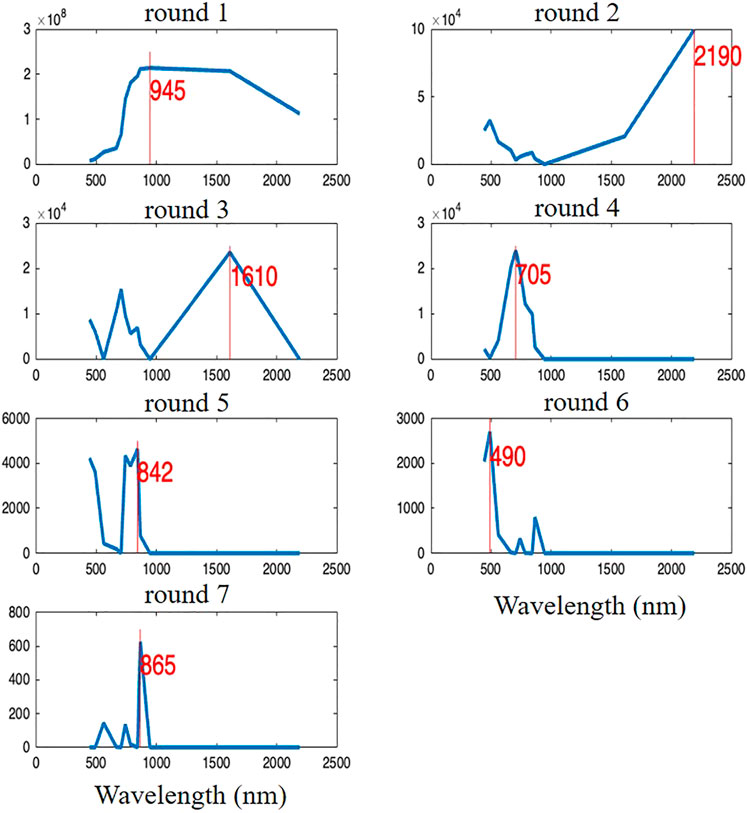
FIGURE 8. Evolution curves of ${\mathrm{cov}}^2\left({\mathrm{X}}_k,\mathrm{y}\right)$ as the first seven spectral slices were selected by N-CovSel algorithm. The selected feature corresponds to the maximum of each curve; the corresponding wavelengths are shown in red.

Each subplot (round) showed clear peaks, allowing the identification of wavelengths involved in the prediction of yield losses. It should be noted that, for each round, the N-CovSel algorithm highlighted a different wavelength of the spectrum. As mentioned for Figure 7, the particularities also shown in Figure 8 ensure at most complementarity.

It was noted that in round 1 (945 nm), the spectrum shown was the average spectrum of the vegetation. Although Clevers et al. (2008) determined that when looking through the atmosphere, the water band absorptions in the 940 nm region should be considered to obtain information on the canopy water content, the shape of the displayed spectrum suggests that the 945 nm spectral band represents more of a multiplicative effect in the data. The 945 nm wavelength region had the highest covariance, i.e., the highest overall reflectance intensity, and this is the reason why the algorithm selected and sorted it in the first round. Regarding the spectral slices selected in the second and third rounds, with the range between 1,600 and 2,500 nm, i.e., in the shortwave infrared (SWIR) domain, it is well-known that the reflectance in this region of the spectrum is strongly correlated with vegetation water content (Jopia et al., 2020; Holzman et al., 2021). However, the second round (2,190 nm) showed a baseline additive-type trend profile that reveals, as the first round, possible effects derived from the remote sensing spectral measurement. It should be noted that these determinations of possible effects do not mean that the two rounds cannot provide information that could explain the changes in water concentration in the vineyard blocks. The following rounds highlighted spectral slices including the red-edge band at 705 nm (round 4) and the near-infrared (NIR) band at 842 and 865 nm (rounds 5 and 7) with round six determining the 490 nm wavelength, known as the blue band. Red-Edge region is related to leaf chlorophyll concentration (Laroche-Pinel et al., 2021) and the reflectance in the NIR region is mainly affected by leaf and canopy structure (Slaton et al., 2001). The higher reflectance at 490 nm may be due to a strong reflection from dead biomass (Lorenzen and Jensen, 1988).

3.3.2 Extraction of 1-D Features

3.3.2.1 Date-Wavelength Columns

Figure 9 shows the operation of the N-CovSel algorithm searching for 1-D features, i.e., pairs of dates-wavelengths. Each sub-plot represents the map of $co{v}^2({\mathrm{x}}_{jk},\mathrm{y})$ as a function of the temporal and spectral domains; the global maximum in each sub-map corresponds to the selected features of X in the second and third dimension with the highest squared covariance with y.

FIGURE 9

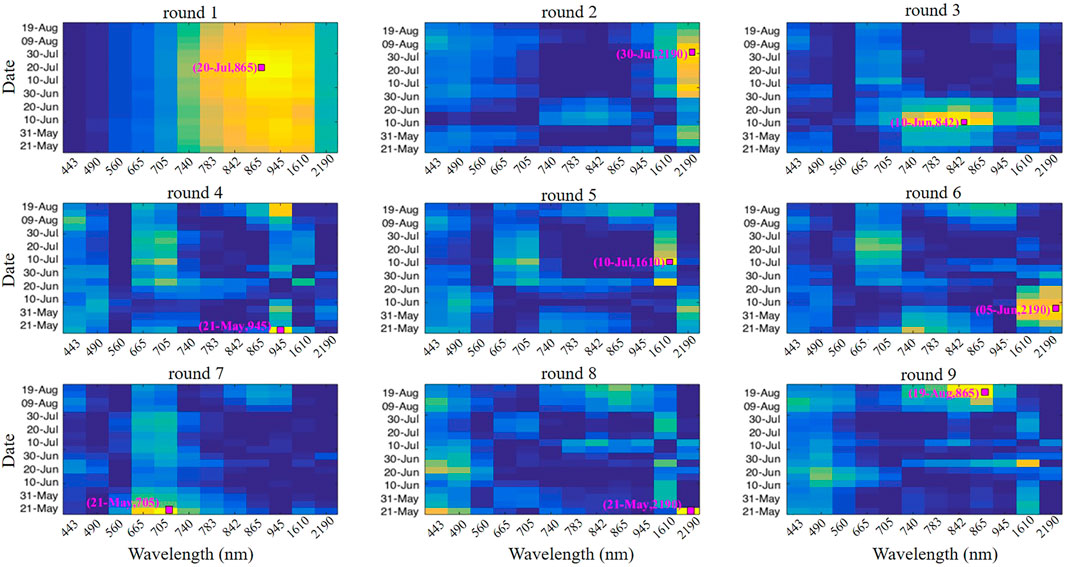
FIGURE 9. Evolution map of ${\mathrm{cov}}^2\left({\mathrm{x}}_{jk},\mathrm{y}\right)$ as the first nine pairs (date-wavelength) selected by N-CovSel. For each of the nine rounds, the date-wavelength selected columns are highlighted by a red square. Dates and wavelengths are texted in pink. The colour gradient represents from yellow to blue, the highest and the lowest values of covariance between the date-wavelength pair (column) and the y-vector respectively.

Each subplot (round) highlighted a different region of the temporal-spectral domain, allowing the identification of date-wavelength pairs involved in predicting yield losses. As for the 2-D extraction, for each round, the information correlated with the previous selected variables was removed, thus significantly decreasing the variance of the neighbouring variables in the following steps (Biancolillo et al., 2022).

The first round, unlike the others, indicates a spectral region as well as consecutive dates, thus determining an overall reflectance effect. It was observed that both the temporal and spectral dimensions had a low frequency, i.e., the N-CovSel algorithm highlighted the entire study period containing the spectral region from 783 to 1,610 nm (yellow). This result indicates that the overall effect of the reflectance, i.e., all-season vegetative profile that was related to the estimation of yield losses observed by the wine growers and advisors by means of maximum values of covariance. The remaining rounds showed high frequencies but in two of the different ways: 1) the second and third rounds showed high frequencies but which were prolonged either in the temporal dimension (round 2) or in the spectral dimension (round 3), For example, focusing on the second round, it should be noticed that the yellow colour appears from the 30th of June, with a maximum peak on the 30th of July but lengthening the high frequency until the 9th of August, at the wavelength 2,190 nm; 2) the remaining rounds from the fourth to the ninth, showed high local frequencies, i.e., covariance peaks, which highlighted more clearly a single date paired to a single wavelength.

Regarding the 1-D feature specificity of each round, the second, sixth and eighth rounds highlighted the wavelength 2,190 nm, but with different dates, 30th July (round 2), 5th June (round 6) and 21st May (round 8). Laroche-Pinel et al. (2021) demonstrated that the wavelength 2,190 nm was one of the most discriminating for vine water status monitoring on a large scale. The three widely temporally spaced rounds may have been indicative of different responses of the various vine growth stages to water variation. The SWIR region is known to be sensitive to cell structure and water vegetation content (Huo et al., 2021). The date of 21st May, which also contained the wavelength in the SWIR region, was previously selected by the algorithm in the fourth and seventh rounds with the wavelengths 945 and 705 nm respectively. From the different wavelengths selected for the same date, it was determined that the initial vineyard blocks conditions related to the water status (2,910 nm) as well as their chlorophyll concentration (705 nm) were related to the final yield losses. Besides the above, on this same date (21st May) the wavelength of 945 nm was highlighted. As shown in Figure 8, this wavelength could be representative of a multiplicative effect of the database and not represent agronomic information of interest. Just as the initial conditions of the set study period (May) were selected by the algorithm, so were the conditions at the end of the study period (August). The ninth round highlighted the pair on 19th August and the wavelength 865 nm. Reflectance between 685 and 700 nm has been established as one of the most sensitive for detecting plant stress (Gitelson et al., 1996). The third and fifth rounds were the closest in time to the heat episode that occurred between the 23rd June and the 3rd July 2019. The selected date-wavelength pairs were as follows: 10th June—842 nm (round 3) and 10th July—1,610 nm (round 5). Reflectance at 842 nm is mainly related to leaf internal structure (Raddi et al., 2021). The high reflectance at this wavelength may have indicated a relevant change in morphology and canopy structure. As demonstrated by Raddi et al. (2021), the reflectance around 850 nm increases with season and severe stress factors. Regarding reflectance at 1,610 nm, many studies reported the strong correlation of leaf water content with reflectance at wavelengths ranging from 1,400 to 1900 nm (Champagne et al., 2003; Das et al., 2018). Thus, round 3 (10th June—842 nm) could represent the water restriction (in the absence of irrigation) just before the heat stress during a period of high plant growth in the LR zone. This indicates that water stress in vineyard blocks before an extreme heat episode could have been an aggravating factor for yield loss. Meanwhile, round 5 (10th July—1,610 nm) could represent the subsequent effect of a sudden and strong heatwave on the water status of the vines.

4 Discussion

A generic example of the application of N-CovSel algorithm for variable selection was provided in the form of a time-series study in multispectral images. This paper showed the potential of methods originally developed in the analytical chemistry domain when applied to larger scales, e.g., in the life science domain. The application demonstrated the value of considering the feature reduction approach in the temporal and spectral dimensions for interpretation purposes in order to understand which variables contributed the most in the life science context presented.

In order to predict and estimate yield losses caused by a heat wave on vineyards fields, the N-CovSel algorithm was used. Based on a variable selection procedure according to their global covariance, the contributions of the temporal and spatial parts and their joint effect in the prediction of yield losses were characterised through three regression models. The performance of the models are as follows: for the temporal N-PLS model (r² = 0.62—RMSE = 11%), for the spatial N-PLS model (r² = 0.61—RMSE = 12%) and the temporal-spectral PLS model (r² = 0.63—RMSE = 11%).

From a predictive point of view, Lopez-Fornieles et al. (2022) already demonstrated that the application of the multidirectional regression method such as the N-PLS algorithm is appropiate to characterise and estimate the impact of an extreme event on grapevine. However, the interpretability offered by N-CovSel proved to be a very useful tool for understanding the agronomic processes underlying the spectral response of the crops over the time. It is well documented in the scientific literature that satellite monitoring of interactions between plants and light reflectance, in situations where crops interact with any aspect of their environment (e.g., extreme weather events), results in changes in plant signal (Knipling, 1970; Segarra et al., 2020). The variable selection approach identified the most significant features in a multidirectional environment, i.e., in a 3-way array, by selecting 2-D features (temporal and spectral slices) or 1-D features (date-wavelength columns) to be implemented within the model construction. Previous studies have shown similar results regarding the effects of heat stress from reflectance data in viticulture (Cogato et al., 2019; Lopez-Fornieles et al., 2022), but notably, in the presented approach, the subset of features was selected simultaneously in two dimensions of the satellite information, i.e., temporal and spectral (Lopez-Fornieles et al., 2022). This selection procedure allows not only to identify the most significant wavelengths of the extreme weather episode but also knowledge on its a priori and a posteriori impact by integrating the temporal analysis from the N-way feature selection algorithm.

Since N-CovSel algorithm eliminates the correlation between variables by projecting the data orthogonally to the selected variable for the neighbouring variables in the following steps (Biancolillo et al., 2022), it is ensured that all selected features are at most complementary to each other. Furthermore, it is possible to sort the selected variables from the highest to the lowest covariance related to observed yield losses. From the temporal slices (2-D features) selected and sorted, three important periods were observed that defined the data to be predicted 1) the initial dates of the study period, centred on 21 May, 2) the dates close to the heatwave that occurred between the 23 June and 8 July and 3) the end of period dates, centred on 14–19 August. For the spectral slices (2-D features), the most important wavelengths (maximum covariance values) that were selected are known to be related to water absorption (Segarra et al., 2020) which may be indicative of the water status as the main factor affecting vine development. Wavelengths corresponding to the SWIR domain were observed from the date-wavelength columns (1-D feature) for the following dates ordered from highest to lowest covariance: 30th July—2,190 nm, 10th July—1,610 nm, 5th June—2,190 nm, 21st May—2,190 nm. As reflectance at 2,190 nm is known to be relevant for monitoring vine water status at large spatial scale (Laroche-Pinel et al., 2021), its selection at different dates throughout the study period shows the inconsistency of considering that yield loss is only due heat stress. Indeed, the initial conditions (21st May) of water stress (2,190 nm) (Laroche-Pinel et al., 2021) as well as the information on the characteristics of the plant physiology in the Red Edge (700 nm) (Lopez-Fornieles et al., 2022) were already decisive for the final prediction. Given the proximity of the dates to the extreme weather event and that the detection of severe drought stress is centred at the wavelength 1,610 nm (Cogato et al., 2019), the date-wavelength pair of 10th July—1,610 nm was considered by the N-CovSel algorithm concerning the heatwave episode. The theory that the spectral response of the canopy representing the physiological behaviour of the grapevine, is affected by stress conditions due to fluctuations in ambient temperature, is well demonstrated in scientific literature (Cogato et al., 2021). In the final period of the study (still in full production), although after the collection of ground truth data on the condition of the vineyard blocks after the heatwave, the N-CovSel algorithm emphasised the 19 August—865 nm pair. The reflectance in the Vegetation Red-Edge region (865 nm) is known in the literature as one of the most discriminating bands for water status (Laroche-Pinel et al., 2021). The results of the present analysis confirm, with a variable selection approach, that a combination of SWIR (1,610–2,190 nm) (Das et al., 2018), Red-Edge (705 nm) (Ballester et al., 2018) and Red-edge Vegetation (865 nm) (Maimaitiyiming et al., 2017), is a valuable indicator for monitoring water status (Laroche-Pinel et al., 2021).

The main advantage of using the N-CovSel algorithm for the remote sensing images is that being a methodology adapted for N-way arrays, the temporality and the spectral information are considered simultaneously. In the context of the life science case study, this allowed to establish that the heatwave was not the only explanatory factor of the final yield losses observed by the winegrowers and advisors. By temporally discriminating the most appropriate spectral information to characterise the beginning or end of the development season, as well as extreme events, it was observed that these were the integrating result of a series of factors that were mainly related to water restriction in key periods for plant development.

It is essential to place the results presented in this paper within the reality of multitemporal satellite data as they are sensors that measure reflected energy within several specific bands of the electromagnetic spectrum (Pettorelli et al., 2014). This implies that, as for the field of NIR spectroscopy (Isaksson and Næs, 1988), effects related to the reflectance of the spectrum are present in the analysis. The N-CovSel algorithm allowed the identification of multiplicative and additive effects in the selection of 2-D features. The choice retain the observed effects was taken, as they could be important information in the interpretation of the model (e.g., wavelength 2019 nm). However, their removal at an early stage could have prevented the occurrence of effects in the covariance-based selection, e.g., wavelength 945 nm, mainly dedicated to atmospheric features detection (Verrelst et al., 2012). It should be noted that, due to the type of approach, the model should only be suitable for the year (2019) and the region (LR) considered. Thus, subsequent models remain specific to the learning base used for the calibration and their generalisation to other crops and/or other agricultural regions is rather limited.

Further applications are required before confirming the operational reliability of the N-CovSel method, in particular to provide spectral-temporal features to identify areas with different water restriction dynamics. For this, it will be necessary to complete the results of this study by extending the variable selection analysis to other types of phenomena, both those with a strong temporal evolution (e.g., extreme weather event such as hail) and those without (e.g., water scarcity in summer season), in order to better determine the dynamics of crop development and thus the reasons for its main cause-effects. As it appears that N-Covsel could be an efficient method addressing multiple response cases, an application study-case to be studied would be its direct application to multispectral images, thus taking into account the spatial dimension.

Data Availability Statement

The original contributions presented in the study are included in the article/Supplementary Material, further inquiries can be directed to the corresponding author.

Author Contributions

Conceptualization, EL-F and J-MR; formal analysis, EL-F and J-MR; methodology, BG and J-MR; validation, EL-F and BT; writing—original draft preparation, EL-F and AC; writing—review and editing, EL-F, AC, BT and J-MR; visualization, EL-F and J-MR; supervision, J-MR. All authors have read and agreed to the published version of the manuscript.

Funding

This work was supported by the French National Research Agency under the Investments for the Future Program, referred as ANR-16-CONV-0004.

Conflict of Interest

The authors declare that the research was conducted in the absence of any commercial or financial relationships that could be construed as a potential conflict of interest.

Publisher’s Note

All claims expressed in this article are solely those of the authors and do not necessarily represent those of their affiliated organizations, or those of the publisher, the editors and the reviewers. Any product that may be evaluated in this article, or claim that may be made by its manufacturer, is not guaranteed or endorsed by the publisher.

Acknowledgments

The authors would like to thank Alessandra Biancolillo and Federico Marini and for providing the N-CovSel algorithm.

References

Alam, M. S., Islam, M. N., Bal, A., and Karim, M. A. Hyperspectral Target Detection Using Gaussian Filter and post-processing. Opt. Lasers Eng. (2008) 46:817–822. doi:10.1016/j.optlaseng.2008.05.019

CrossRef Full Text | Google Scholar

Ballester, C., Zarco-Tejada, P. J., Nicolás, E., Alarcón, J. J., Fereres, E., Intrigliolo, D. S., et al. Evaluating the Performance of Xanthophyll, Chlorophyll and Structure-Sensitive Spectral Indices to Detect Water Stress in Five Fruit Tree Species. Precision Agric. (2018) 19:178–193. doi:10.1007/s11119-017-9512-y

CrossRef Full Text | Google Scholar

Biancolillo, A., Marini, F., and Roger, J. M. N-CovSel, a New Strategy for Feature Selection in N-Way Data. In: 17th Scandinavian Symposium of Chemometrics (SSC17); September 2021; Aalborg (DK) (2021). 6–9. https://ssc17.org/Program_abstracts.pdf

Google Scholar

Bishop, M. P. 3.1 Remote Sensing and GIScience in Geomorphology: Introduction and Overview. In: J. F. Shroder, editor. 3.1 Remote Sensing and GIScience in Geomorphology: Introduction and OverviewTreatise on Geomorphology. San Diego: Academic Press (2013). 1–24. doi:10.1016/B978-0-12-374739-6.00040-3

CrossRef Full Text | Google Scholar

Bro, R. Multiway Calibration. Multilinear PLS. J. Chemometrics (1996) 10:47–61. doi:10.1002/(sici)1099-128x(199601)10:1<47::aid-cem400>3.0.co;2-c

CrossRef Full Text | Google Scholar

Champagne, C. M., Staenz, K., Bannari, A., McNairn, H., and Deguise, J.-C. Validation of a Hyperspectral Curve-Fitting Model for the Estimation of Plant Water Content of Agricultural Canopies. Remote Sensing Environ. (2003) 87:148–160. doi:10.1016/S0034-4257(03)00137-8

CrossRef Full Text | Google Scholar

Clevers, J. G. P. W., Kooistra, L., and Schaepman, M. E. Using Spectral Information from the NIR Water Absorption Features for the Retrieval of Canopy Water Content. Int. J. Appl. Earth Observation Geoinformation (2008) 10:388–397. doi:10.1016/j.jag.2008.03.003

CrossRef Full Text | Google Scholar

Cogato, A., Pagay, V., Marinello, F., Meggio, F., Grace, P., and De Antoni Migliorati, M. Assessing the Feasibility of Using Sentinel-2 Imagery to Quantify the Impact of Heatwaves on Irrigated Vineyards. Remote Sensing (2019) 11:2869. doi:10.3390/rs11232869

CrossRef Full Text | Google Scholar

Cogato, A., Wu, L., Jewan, S. Y. Y., Meggio, F., Marinello, F., Sozzi, M., et al. Evaluating the Spectral and Physiological Responses of Grapevines (Vitis vinifera L.) to Heat and Water Stresses under Different Vineyard Cooling and Irrigation Strategies. Agronomy (2021) 11:1940. doi:10.3390/agronomy11101940

CrossRef Full Text | Google Scholar

Coppi, R. An Introduction to Multiway Data and Their Analysis. Comput. Stat. Data Anal. (1994) 18:3–13. doi:10.1016/0167-9473(94)90130-9

CrossRef Full Text | Google Scholar

Das, B., Mahajan, G. R., and Singh, R. Hyperspectral Remote Sensing: Use in Detecting Abiotic Stresses in Agriculture. In: S. K. Bal, J. Mukherjee, B. U. Choudhury, and A. K. Dhawan, editors. Advances in Crop Environment Interaction. Singapore: Springer Singapore (2018). p. 317–335. doi:10.1007/978-981-13-1861-0_12

CrossRef Full Text | Google Scholar

de Juan, A., and Tauler, R. Data Fusion by Multivariate Curve Resolution. In: M. Cocchi, editor. Data Handling in Science and Technology Data Fusion Methodology and Applications. Elsevier (2019). p. 205–233. doi:10.1016/B978-0-444-63984-4.00008-9

CrossRef Full Text | Google Scholar

Devaux, N., Crestey, T., Leroux, C., and Tisseyre, B. Potential of Sentinel-2 Satellite Images to Monitor Vine fields Grown at a Territorial Scale. OENO One (2019) 53. doi:10.20870/oeno-one.2019.53.1.2293

CrossRef Full Text | Google Scholar

Favilla, S., Durante, C., Vigni, M. L., and Cocchi, M. Assessing Feature Relevance in NPLS Models by VIP. Chemometrics Intell. Lab. Syst. (2013) 129:76–86. doi:10.1016/j.chemolab.2013.05.013

CrossRef Full Text | Google Scholar

Filella, I., Serrano, L., Serra, J., and Peñuelas, J. Evaluating Wheat Nitrogen Status with Canopy Reflectance Indices and Discriminant Analysis. Crop Sci. (1995) 35:1400–1405. doi:10.2135/cropsci1995.0011183X003500050023x

CrossRef Full Text | Google Scholar

Gitelson, A. A., Kaufman, Y. J., and Merzlyak, M. N. Use of a green Channel in Remote Sensing of Global Vegetation from EOS-MODIS. Remote Sensing Environ. (1996) 58:289–298. doi:10.1016/S0034-4257(96)00072-7

CrossRef Full Text | Google Scholar

Henrion, R. N-way Principal Component Analysis Theory, Algorithms and Applications. Chemometrics Intell. Lab. Syst. (1994) 25:1–23. doi:10.1016/0169-7439(93)E0086-J

CrossRef Full Text | Google Scholar

Hollstein, A., Segl, K., Guanter, L., Brell, M., and Enesco, M. Ready-to-Use Methods for the Detection of Clouds, Cirrus, Snow, Shadow, Water and Clear Sky Pixels in Sentinel-2 MSI Images. Reote Sensing (2016) 8:666. doi:10.3390/rs8080666

CrossRef Full Text | Google Scholar

Holzman, M. E., Rivas, R. E., and Bayala, M. I. Relationship between TIR and NIR-SWIR as Indicator of Vegetation Water Availability. Remote Sensing (2021) 13:3371. doi:10.3390/rs13173371

CrossRef Full Text | Google Scholar

Hong, D., Gao, L., Yao, J., Zhang, B., Plaza, A., and Chanussot, J. Graph Convolutional Networks for Hyperspectral Image Classification. IEEE Trans. Geosci. Remote Sensing (2020) 59(7):5966–5978.

Google Scholar

Huo, L., Persson, H. J., and Lindberg, E. Early Detection of forest Stress from European spruce Bark Beetle Attack, and a New Vegetation index: Normalized Distance Red & SWIR (NDRS). Remote Sensing Environ. (2021) 255:112240. doi:10.1016/j.rse.2020.112240

CrossRef Full Text | Google Scholar

Isaksson, T., and Næs, T. The Effect of Multiplicative Scatter Correction (MSC) and Linearity Improvement in NIR Spectroscopy. Appl. Spectrosc. (1988) 42:1273–1284. doi:10.1366/0003702884429869

CrossRef Full Text | Google Scholar

Jopia, A., Zambrano, F., Pérez-Martínez, W., Vidal-Páez, P., Molina, J., and de la Hoz Mardones, F. Time-Series of Vegetation Indices (VNIR/SWIR) Derived from Sentinel-2 (A/B) to Assess Turgor Pressure in Kiwifruit. Ijgi (2020) 9:641. doi:10.3390/ijgi9110641

CrossRef Full Text | Google Scholar

Knipling, E. B. Physical and Physiological Basis for the Reflectance of Visible and Near-Infrared Radiation from Vegetation. Remote Sensing Environ. (1970) 1:155–159. doi:10.1016/S0034-4257(70)80021-9

CrossRef Full Text | Google Scholar

Laroche-Pinel, E., Duthoit, S., Albughdadi, M., Costard, A. D., Rousseau, J., Chéret, V., et al. Towards Vine Water Status Monitoring on a Large Scale Using Sentinel-2 Images. Remote Sensing (2021) 13:1837. doi:10.3390/rs13091837

CrossRef Full Text | Google Scholar

Liu, Y., Hiyama, T., Kimura, R., and Yamaguchi, Y. Temporal Influences on Landsat‐5 Thematic Mapper Image in Visible Band. Int. J. Remote Sensing (2006) 27:3183–3201. doi:10.1080/01431160600647258

CrossRef Full Text | Google Scholar

Lopez-Fornieles, E., Brunel, G., Rancon, F., Gaci, B., Metz, M., Devaux, N., et al. Potential of Multiway PLS (N-PLS) Regression Method to Analyse Time-Series of Multispectral Images: A Case Study in Agriculture. Remote Sensing (2022) 14:216. doi:10.3390/rs14010216

CrossRef Full Text | Google Scholar

Lorenzen, B., and Jensen, A. Reflectance of Blue, green, Red and Near Infrared Radiation from Wetland Vegetation Used in a Model Discriminating Live and Dead above Ground Biomass. New Phytol. (1988) 108:345–355. doi:10.1111/j.1469-8137.1988.tb04173.x

PubMed Abstract | CrossRef Full Text | Google Scholar

Maimaitiyiming, M., Ghulam, A., Bozzolo, A., Wilkins, J. L., and Kwasniewski, M. T. Early Detection of Plant Physiological Responses to Different Levels of Water Stress Using Reflectance Spectroscopy. Remote Sensing (2017) 9:745. doi:10.3390/rs9070745

CrossRef Full Text | Google Scholar

Mehmood, T., Liland, K. H., Snipen, L., and Sæbø, S. A Review of Variable Selection Methods in Partial Least Squares Regression. Chemometrics Intell. Lab. Syst. (2012) 118:62–69. doi:10.1016/j.chemolab.2012.07.010

CrossRef Full Text | Google Scholar

Pettorelli, N., Laurance, W. F., O'Brien, T. G., Wegmann, M., Nagendra, H., and Turner, W. (2014). Satellite Remote Sensing for Applied Ecologists: Opportunities and Challenges. J. Appl. Ecol. 51, 839–848. doi:10.1111/1365-2664.12261

CrossRef Full Text | Google Scholar

Pettorelli, N., Laurance, W. F., and O'Brien, T. G. N-CovSel, a New Strategy for Feature Selection in N-Way Data (2022). Submitted to Analytica Chimica Acta.

Google Scholar

Picoli, M. C. A., Simoes, R., Chaves, M., Santos, L. A., Sanchez, A., Soares, A., et al. CBERS Data Cube: a Powerful Technology for Mapping and Monitoring Brazilian Biomes. ISPRS Ann. Photogramm. Remote Sens. Spat. Inf. Sci. (2020) 3:533–539. doi:10.5194/isprs-annals-V-3-2020-533-2020

CrossRef Full Text | Google Scholar

Raddi, S., Giannetti, F., Martini, S., Farinella, F., Chirici, G., Tani, A., et al. Monitoring Drought Response and Chlorophyll Content in Quercus by Consumer-Grade, Near-Infrared (NIR) Camera: a Comparison with Reflectance Spectroscopy. New Forests (2021) 53:241–265. doi:10.1007/s11056-021-09848-z

CrossRef Full Text | Google Scholar

Raza, A., Razzaq, A., Mehmood, S., Zou, X., Zhang, X., Lv, Y., et al. Impact of Climate Change on Crops Adaptation and Strategies to Tackle its Outcome: A Review. Plants (2019) 8:34. doi:10.3390/plants8020034

PubMed Abstract | CrossRef Full Text | Google Scholar

R. E. Plant, R. E., D. S. Munk, D. S., B. R. Roberts, B. R., R. L. Vargas, R. L., D. W. Rains, D. W., R. L. Travis, R. L., et al. Relationships between Remotely Sensed Reflectance Data and Cotton Growth and Yield. Trans. ASAE (2000) 43:535–546. doi:10.13031/2013.2733

CrossRef Full Text | Google Scholar

Richter, K., Hank, T. B., Vuolo, F., Mauser, W., and D’Urso, G. Optimal Exploitation of the Sentinel-2 Spectral Capabilities for Crop Leaf Area Index Mapping. Remote Sensing (2012) 4:561–582. doi:10.3390/rs4030561

CrossRef Full Text | Google Scholar

Roger, J. M., Palagos, B., Bertrand, D., and Fernandez-Ahumada, E. CovSel: Variable Selection for Highly Multivariate and Multi-Response Calibration. Application to IR Spectroscopy. Chemometrics Intell. Lab. Syst. (2011) 106:216–223. doi:10.1016/j.chemolab.2010.10.003

CrossRef Full Text | Google Scholar

Salvatore, E., Bevilacqua, M., Bro, R., Marini, F., and Cocchi, M. Classification Methods of Multiway Arrays as a Basic Tool for Food PDO Authentication. In: Comprehensive Analytical Chemistry. Elsevier (2013). 339–382. doi:10.1016/B978-0-444-59562-1.00014-1

CrossRef Full Text | Google Scholar

Schymanski, S. J., Or, D., and Zwieniecki, M. Stomatal Control and Leaf Thermal and Hydraulic Capacitances under Rapid Environmental Fluctuations. PLOS ONE (2013) 8:e54231. doi:10.1371/journal.pone.0054231

PubMed Abstract | CrossRef Full Text | Google Scholar

Segarra, J., Buchaillot, M. L., Araus, J. L., and Kefauver, S. C. Remote Sensing for Precision Agriculture: Sentinel-2 Improved Features and Applications. Agronomy (2020) 10:641. doi:10.3390/agronomy10050641

CrossRef Full Text | Google Scholar

Slaton, M. R., Raymond Hunt, E., and Smith, W. K. Estimating Near-Infrared Leaf Reflectance from Leaf Structural Characteristics. Am. J. Bot. (2001) 88:278–284. doi:10.2307/2657019

PubMed Abstract | CrossRef Full Text | Google Scholar

Trevino, V., and Falciani, F. GALGO: an R Package for Multivariate Variable Selection Using Genetic Algorithms. Bioinformatics (2006) 22:1154–1156. doi:10.1093/bioinformatics/btl074

PubMed Abstract | CrossRef Full Text | Google Scholar

Venios, X., Korkas, E., Nisiotou, A., and Banilas, G. Grapevine Responses to Heat Stress and Global Warming. Plants (2020) 9:1754. doi:10.3390/plants9121754

CrossRef Full Text | Google Scholar

Verrelst, J., Muñoz, J., Alonso, L., Delegido, J., Rivera, J. P., Camps-Valls, G., et al. Machine Learning Regression Algorithms for Biophysical Parameter Retrieval: Opportunities for Sentinel-2 and -3. Remote Sensing Environ. (2012) 118:127–139. doi:10.1016/j.rse.2011.11.002

CrossRef Full Text | Google Scholar

Wold, S., Sjöström, M., and Eriksson, L. PLS-regression: A Basic Tool of Chemometrics. Chemometrics Intell. Lab. Syst. (2001) 58:109–130. doi:10.1016/S0169-7439(01)00155-1

CrossRef Full Text | Google Scholar