Energy-Efficient Mobility Prediction Routing Protocol for Freely Floating Underwater Acoustic Sensor Networks

Introduction

Motivated by the wish to provide autonomous support for several underwater applications, underwater acoustic sensor networks (UASNs) have gained remarkable momentum within the research community in the last few years. However, the unique characteristics of the underwater channel (Zorzi et al., 2008; Zhang et al., 2010; Rahman et al., 2012; Coutinho et al., 2016; Wang et al., 2018) impose severe challenges such as high attenuation, limited bandwidth, long propagation delay, and especially high transmission power, while sensors’ energy budget is not only limited but also cannot be easily recharged. Thus, UASNs require novel energy-efficient protocols that take into account the characteristics of underwater environments to meet monitoring application requirements. Proposing an energy-efficient data forwarding protocol that makes judicious use of the limited energy budget is crucial as it is responsible for setting a whole path from the source to the sink in a freely floating underwater sensor network.

To successfully design a data forwarding protocol for UASNs, two issues need to be carefully addressed since they highly affect the performance of the data forwarding protocols, namely, i) how to take into account the mobility of freely floating sensor nodes in dynamic underwater environments to forward one data packet through one single best path without the need to exchange notification messages and ii) what are the forwarder selection criteria to select the best forwarder along the path among all the available ones. To address the first issue, designing a data forwarding protocol based on a realistic, physically inspired mobility model that captures the dynamics of underwater nodes is crucial. In other words, using a realistic mobility model helps to predict the best path to the sink at the source node level. To handle the second issue, the data forwarding protocol should choose the best path based on the remaining energy of future neighboring nodes. To address both issues, we propose a mobility prediction optimal data forwarding protocol. To the best of our knowledge, an MPODF protocol is the first data forwarding protocol that takes into account the realistic mobility pattern of freely floating sensor nodes to predict the best energy-efficient path toward the sink and hence avoid notification messages’ exchange to establish a path.

Our contributions can be summarized as follows. First, we consider a realistic, physically inspired mobility model that meticulously captures the dynamics of underwater nodes under the water current forces, the gravitational force, the buoyant force, and the water resistance. This mobility model was proposed by Bouabdallah (2019) and not only considers all the physical forces but also most of the underwater characteristics such as salinity, tide, and bathymetry. Second, using this mobility model, we propose a prediction-based routing protocol MPODF. MPODF is a source routing protocol that predicts the best energy-efficient path to the sink to deliver a data packet. It is worth pointing out that MPODF predicts and uses a single path without exchanging any extra notification packets to set a path. Finally, the performance of MPODF was evaluated under high-mobility scenarios where the flooding protocol is among the most efficient and usable protocol. Indeed, when the sensors are mobile with a high speed, the flooding protocol becomes the unique efficient solution to deliver packets to a far sink. A performance evaluation shows that MPODF outperforms the flooding protocol, especially in terms of energy efficiency.

This article is organized as follows. First, in Related Work, we review some works related to routing protocols in freely floating UASNs. In Problem Statement, we explain the problem statement. In Mobility Model, we thoroughly describe the mobility model. In MPODF Protocol, we describe the design of the MPODF protocol with all its features and its prediction processes in detail. In Performance Evaluation, we evaluate the performance of our proposed mobility prediction optimal data forwarding (MPODF) protocol. Finally, in Conclusion, we conclude this article with a summary of our contributions.

Related Work

There have been many research works to address the data forwarding protocols for UASNs, especially for freely floating underwater sensors (Hwang and Kim, 2008; Ayaz and Abdullah, 2009; Xie et al., 2009; Ayaz et al., 2010; Baccour et al., 2010; Liu and Li, 2010).

Based on the routing strategy and the major parameters it utilizes for routing purposes, UASN routing can be classified into reliable data forwarding protocols (Nicolaou et al., 2007; Yan et al., 2008; Ayaz and Abdullah, 2009; Wahid et al., 2014; Noh et al., 2016) and predication-based data forwarding protocols (Ayaz and Abdullah, 2009; Wahid and Kim, 2012; Chen and Lin, 2013; Jafri et al., 2013; Wei et al., 2013; Jafri et al., 2014; Khan et al., 2015; Umar et al., 2015).

Reliable Data Forwarding Protocols

Reliable data forwarding protocols mainly focus on providing guaranteed delivery of data packets over unreliable UASNs by forwarding through multiple paths (Xie et al., 2009; Wahid and Kim, 2012; Jafri et al., 2013; Jafri et al., 2014; Wahid et al., 2014; Ibrahim et al., 2014). The reliable data forwarding protocols’ class can be further divided into two subclasses, namely, location-based data forwarding protocols and depth-based data forwarding protocols.

Location-Based Data Forwarding Protocols

In the location-based data forwarding protocol, such as Xie et al. (2006), the packet forwarding route is specified by predefining a virtual pipe from the source node to the sink node, where only the nodes within the radius of the virtual pipe participate in the forwarding process of the data packets. However, the selection process of the next forwarders is sensitive to the radius of the virtual pipe which will impact the number of potential forwarders in the virtual pipe, and hence, the performance of the protocol is affected.

In Nicolaou et al. (2007), the protocol is designed to overcome the Xie et al. (2006) performance sensitivity to the radius of the “virtual pipe.” Different from Xie et al. (2006), when a node receives a data packet, the receiving node calculates the virtual pipe from itself to the sink node, and the process is repeated at each receiving node. So, the forwarding path changes at each receiving node toward the sink. However, recomputing the routing pipe on each hop increases the computational delay and affects the overall network throughput.

Depth-Based Data Forwarding Protocols

In depth-based data forwarding protocols, such as Yan et al. (2008), the selection of the next forwarder node relies mainly on its depth. Indeed, if the next forwarder depth is less than the current forwarder depth, then the next forwarder will proceed to send the data packet. However, the protocol proposed in Yan et al. (2008) suffers from a low delivery ratio in a low-density network.

Prediction-Based Data Forwarding Protocols

Prediction-based data forwarding protocols predict nodes’ future movement patterns due to the tides, ocean currents, and other environmental forces that help to estimate and calculate the location and coverage probability for each node without the help of any localization technique (Ahmed et al., 2017; Coutinho et al., 2016; Coutinho et al., 2018; Dhurandher et al., 2018; Han et al., 2019). The prediction-based data forwarding protocols can be further divided into two subclasses, namely, mobility model-based data forwarding protocols and filter-based data forwarding protocols.

Mobility Model-Based Data Forwarding Protocols

In mobility model-based data forwarding protocols, such as Nowsheen et al. (2014), every node estimates its own location and its coverage probability and predicts its future movement pattern in the absence of any localization technique. In Nowsheen et al. (2014), the mobility prediction data forwarding protocol, MPDF, is proposed where each possible candidate forwarder exchanges multiple notification messages with the downstream node and calculates three parameters: link reachability, uplink transmission reliability, and coverage probability. The neighbor with the highest coverage probability, the best uplink transmission reliability, and the best link reachability will be selected as the next-hop forwarder. MPDF suffers from routing overhead and high energy consumption due to the exchange of multiple notification messages at each hop.

In Tian et al. (2010), the nodes’ location, transmission latency, and energy consumption are considered to select the best path to the sink node. It selects the forwarders with dominance in both the spatial dimension and the time dimension to identify several paths from the source to the sink and then assign a probability to each path that is based on the nodes’ residual energy in each path. The protocol proposed in Tian et al. (2010) has a high successful packet rate and energy effectiveness; however, it is not suitable for real-time networks as it suffers from higher transmission delay due to the calculation load in space, time, and energy aspects for the forwarding candidates.

Filter-Based Data Forwarding Protocols

A filter-based data forwarding protocol is proposed in Hu and Fei (2013). It is based on Q-learning which is a distributed machine learning technique. Accordingly, an adaptive filter is used which is able to learn and predict future contact probabilities and make the data forwarding decisions which are whether to forward data packets to the present neighbor node in contact or to wait for the next neighbor node in contact. Despite its robustness, it broadcasts multiple beacon packets for the purpose of neighbor discoveries that result in high energy consumption.

Table 1 compares all the described protocols.

TABLE 1

TABLE 1. Comparison among related work protocols.

TABLE 2

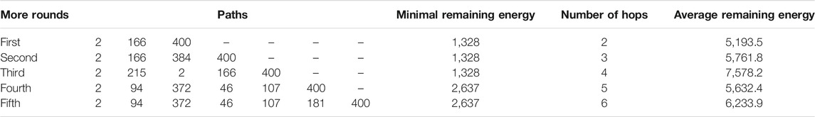
TABLE 2. More rounds for node 2.

In this article, we proposed a mobility-based data forwarding protocol that aims at finding the best energy-efficient path without exchanging any extra packets to set a path. Indeed, by using a realistic, physically inspired mobility model that predicts the future movement of every node, the best path can be accurately estimated.

Problem Statement

Providing efficient and reliable data forwarding services in underwater sensor networks is very challenging due to the unique characteristics of the UASN environment. The freely floating sensor nodes in UASNs move according to water currents, resulting in a highly dynamic network topology.

The existing data forwarding protocols for UASNs need to update the routing information periodically by extensively exchanging notification messages, which results in significant energy consumption and communication overhead. Accordingly, the performance of all the proposed data forwarding protocols for UASNs dramatically decreases if we take into account the realistic mobility pattern of freely floating sensor nodes subject to the water current and other aquatic environment forces.

To manage the dynamic topology, we consider a realistic mobility pattern that mimics the trajectory of freely floating sensor nodes. This mobility model is proposed in Bouabdallah (2019) and remarkably not only considers the water current forces but also all the other underwater forces that impact the trajectory of the freely floating underwater sensor. Note that, in Bouabdallah (2019), a realistic, physically inspired mobility model is proposed that meticulously captures the dynamics of underwater nodes under the water current forces, the gravitational force, the buoyant force, and the water resistance.

Based on this mobility model derived in Bouabdallah (2019), we propose a mobility prediction data forwarding (MPODF) protocol for UASNs that aims at predicting the best path to the sink from the source node level. By doing so, the source node will be able to choose the best path under the harsh mobility constraint without exchanging extra signaling messages among intermediate nodes to set a path and without crossing multiple paths in order to guarantee delivery to the sink. Therefore, further energy conservation is achieved.

Mobility Model

The network topology in an underwater environment is constantly varying due to node mobility with respect to water currents and water pressure (Ahmed et al., 2017). Indeed, the performance of all the data forwarding protocols for UASNs may dramatically decrease, especially for freely floating underwater sensors, if we neglect the mobility effects. In addition, the use of a global positioning system (GPS) is inapplicable and expensive in underwater environments. Indeed, using GPS is not possible due to the 1.5 GHz radio frequency adopted by the GPS, which can be rapidly absorbed in water.

Consequently, understanding and considering the mobility features of a freely floating underwater sensor are needed to design efficient networking protocols for UASNs.

Our MPODF protocol is based on the mobility model derived in Bouabdallah (2019). Note that, in Bouabdallah (2019), a realistic, physically inspired mobility model is proposed that meticulously captures the dynamics of randomly scattered underwater freely floating sensor nodes under the water current forces, the gravitational force, the buoyant force, and the water resistance. This mobility model not only provides a clearer understanding of all the physical forces applied to a freely floating underwater sensor but also helps to conceive efficient communication protocols.

According to this mobility model, the first force to be considered is the weight of the node ${\overrightarrow{F}}_W$, which is as follows:

${\overrightarrow{F}}_W=p_s{V}_s\overrightarrow{g},(1)$

where $p_s$ is the density of the sensor, $V_s$ is the volume of the sensor, and $\overrightarrow{g}$ is the acceleration of the terrestrial gravity. The weight force makes the sensor accelerate downwards. It is the principal force that sinks the nodes.

The second force is the buoyant force ${\overrightarrow{F}}_B$, which is countering the weight force and equals the weight of displaced water, which reads as follows:

${\overrightarrow{F}}_B=-p_w{V}_s\overrightarrow{g},(2)$

where $p_w$ is the density of water that depends on the depth of water. If the density of the sensor is higher than the density of water, the buoyant force is exceeded by the weight, and the sensor sinks down. The sensor’s weight is constant, while the buoyant force increases with the water depth as the sensor sinks. At a certain depth, the density of water can be equal to the density of the sensor, and as a result, the buoyant force balances the sensor weight. Therefore, the water depth will be asymptotic of the z-coordinate sensor value.

However, the third and fourth forces depend on the kinematics of the sensor. In other words, the third and fourth forces depend on the sensor and water velocities. The third force is the force that the water current applies to thrust the sensor in the same direction as the water stream which reads as follows:

${\overrightarrow{F}}_C=C\sigma A_C\left({\overrightarrow{v}}_C-{\overrightarrow{v}}_{\mathrm{∕∕}}\right),(3)$

where $C$ is a constant, $\sigma$ is a shape factor, $A_C$ is the sensor cross-section area facing the current, ${\overrightarrow{v}}_C$ is the water current velocity, and ${\overrightarrow{v}}_{\mathrm{∕∕}}$ is the sensor’s velocity. The water current force is the only force that controls the horizontal movement of the sensor. The horizontal motion of the sensor vanishes as the velocity of the sensor tends to equal the current’s velocity.

The fourth and last force is the water resistance’s force that is normally applied to the current velocity level. It is written as follows:

${\overrightarrow{F}}_R=-k p_{w}u{A}_R\left({\overrightarrow{v}}_C-{\overrightarrow{v}}_{\mathrm{∕∕}}\right),(4)$

where k is a constant, $u$ is a shape factor, and $A_R$ is the sensor’s cross section perpendicular to the current. The water resistance’s force tends to prevent the horizontal movement of the sensor perpendicular to the water current. The forces of weight, buoyant, and water resistance govern the vertical motion. The free-body diagram is shown in Figure 1.

FIGURE 1

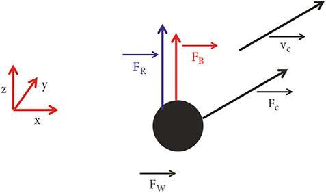
FIGURE 1. Free-body diagram (Bouabdallah, 2019).

In Figure 2, the sensor nodes disperse along the x-, y-, and z-axis, which shows the nodes’ displacements with the water currents.

FIGURE 2

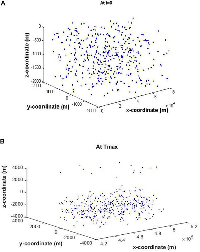
FIGURE 2. The positions of 400 sensors at (A) time = 0 and (B) after 5 days.

Figure 2A shows the positions of 400 sensors right after the deployment, and Figure 2B shows the outcomes of the temporal impact of the mobility model on sensor nodes’ dispersion after 5 days.

By knowing the sensors’ initial position and the velocity of the water current, a time incremental procedure can be used to calculate and determine the location and velocity of any sensor at any time. This procedure can be repeated independently for each sensor to acquire time positions of all sensors in the network.

As explained previously, our MPODF protocol for UASNs is based on mobility prediction. Accordingly, the MPODF protocol uses the calculated time positions of all the sensors provided by the mobility model to predict the best path to the sink at the source node level. Based on the mobility model, the MPODF protocol will be able to discover a single best path to the sink in freely floating sensor node networks without using any localization techniques. Moreover, our MPODF protocol is expected to be energy efficient as it succeeds to forward a single data packet through a single path (no redundancy) without any extra notification packet which will increase the lifetime of the network. The mobility model helps the protocol to select the right candidate forwarder along the optimal path toward the sink.

MPODF Protocol

MPODF is a data forwarding protocol for freely floating UASNs based on a mobility prediction model. MPODF is a routing protocol that forwards one data packet through one single best path without the need to exchange notification messages at each hop to select the optimal and the best next hop in the absence of any localization technique. In other words, MPODF is a source routing protocol according to which the source node is responsible for determining the whole path to the sink, and hence, intermediate nodes will be in charge of simply applying the path. Each sensor node having a data packet to send uses the mobility model in Bouabdallah (2019) to predict the future movement of its one-hop neighbors. In addition to this, it also predicts the far-future movement of its two-hop neighbors, and so on, till reaching the sink, and hence, the best path is selected. In other words, for every potential intermediate node, the protocol tries to find out the eligible next-hop forwarder that will remain within its transmission range during the transmission time. A further detailed description is provided in the next section.

Neighbors’ Prediction Process

A continuous node movement makes it difficult to handle the location information of sensor nodes. Indeed, identifying and discovering the node location in the dynamic underwater environment is a challenging task. The mobility model described in Mobility Model is used as a solution to predict the position of nodes in a specific future time.

A given node is considered an eligible neighbor when it remains moving within the communication range of a sender node during data transmission. More precisely, a pair of nodes $n_1$ and $n_2$, initially placed at a random distance d0, as they are randomly deployed, will move relative to each other according to the previously explained mobility model, resulting in a varying distance between them, $d(t$) as a function of time. $n_1$ is considered a neighbor to $n_2$ if and only if the average distance between them during the reception time, which is the beginning of the transmission till the reception of the packet, is less than the sender transmission range. In this case, the packet will be successfully received. Note that the reception time starts at $T_{propagation}$ after the beginning of the transmission and ends at $T_{transmission}$ later. In other words, if $t$ is the start time of the transmission, the reception interval is $\left[t+T_{propagation},t+T_{propagation}+T_{transmission}\right]$ where $T_{propagation}=\frac{d\left(t\right)}{speed\mathit{a}cousticwave}$ is the propagation time between $n_1$ and $n_2$ and $T_{transmission}$ is the transmission time of the data packet. $T_{transmission}=\frac{packetsize}{linkcapacity}$. Note that $d\left(t\right)$ is the distance at time t between $n_1$ and $n_2$, and $speed\mathit{a}cousticwave$ equals 1500 m/s.

According to the mobility model, every node, namely, $n_1$ and $n_2$, will have a timely position $\left(x_1\left(t\right),y_1\left(t\right),z_1\left(t\right)\right)$ and $\left(x_2\left(t\right),y_2\left(t\right),z_2\left(t\right)\right)\text{ ,}$ respectively.

In order to determine if $n_1$ is in the transmission range of $n_2$ at a given time $t$,the following equation is used:

$d\left(t\right)=\sqrt{{\left(x_1\left(t\right)-x_2\left(t\right)\right)}^2+{\left(y_1\left(t\right)-y_2\left(t\right)\right)}^2+{\left(z_1\left(t\right)-z_2\left(t\right)\right)}^2}.(5)$

In order to decide if $n_2$ is a potential next-hop forwarder of $n_1$, we calculate the average distance between them during $\left[t+T_{propagation},t+T_{propagation}+T_{transmission}\right]$. If the average distance during this reception time is less than the sensor communication range, then $n_2$ will be considered a potential next-hop forwarder of $n_1$. Otherwise, the nodes are drifted apart, and hence, even if initially $n_2$ was a neighbor of $n_1$ at time$t$, $n_2$ will not be considered a potential next-hop forwarder of $n_1$. Consequently, $n_2$ will not be in the selection process of the best next-hop forwarder of $n_1$ as it will be explained in the next section.

Predicting Paths to the Sink

The MPODF protocol starts at time t when the source node has a data packet to be sent to the sink node. The source node activates the prediction module using the mobility model that is proposed in Bouabdallah (2019) to find out the best path to the sink. In more detail, at the first step, the source node starts by predicting its one-hop neighbors during the time $\left[t+T_{propagation},t+T_{propagation}+T_{transmission}\right]$ as explained in the previous section. Call $T_s$ the sum of $T_{propagation}$ and $T_{transmission}$:

$T_s=T_{propagation}+T_{transmission}.$

After predicting its neighbors, at the second step, the source node predicts the neighbors of each one of its previously determined 1-hop neighbors during the time $\left[t+T_s,t+2T_s\right]$. Continuously, the sender at step $\left(n\right)$ keeps predicting the neighbors of each previously predicted $\left(n-1\right)$-hop away neighbors during the time interval $\left[t+\left(n-1\right)T_s,t+\left(n\right)T_s\right]$, and so forth, until the sink node shows up in the timely built predicted graph, as illustrated in Figure 3. Consequently, the source node will succeed in predicting all the paths to the sink node. Then, the sender will proceed selecting the best path as it will be explained in the next section. Once done, the selected best path is embedded in the data packet and sent to the selected best forwarder. The intermediate forwarder has to simply apply the route included in the data packet. Figure 3 illustrates the process of selecting the next forwarder node in the MPODF protocol. Figure 4 shows the pseudocode for the MPODF protocol.

FIGURE 3

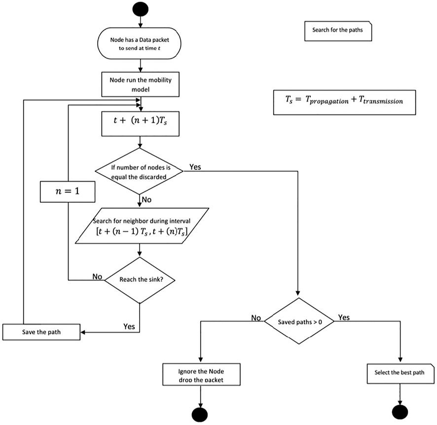
FIGURE 3. The process of selecting the next forwarder node in an MPODF protocol.

FIGURE 4

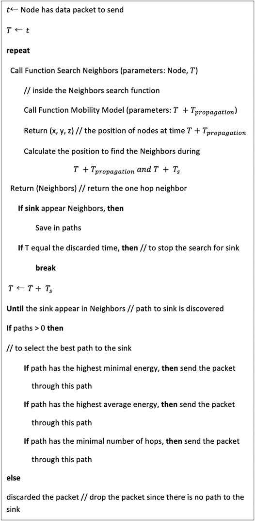
FIGURE 4. The pseudocode for an MPODF protocol.

The More-Round Feature

As explained in the previous section, in order to predict all the possible paths to the sink, the node keeps predicting the future eligible neighbors of its previously determined n-hop away neighbors until reaching the sink. Once the sink shows up in the neighbor’s prediction process, the source node stops the prediction process and starts comparing all the derived possible paths toward the sink in order to extract the best one.

In order to improve the performance of MPODF, we suggest that the source node will continue the prediction process even after the appearance of the sink. By doing so, longer paths in terms of number of hops will be identified with the hope that they may be more energy efficient. The more-round feature in MPODF refers to the number of times the neighbors’ prediction process is executed after reaching the sink for the first time. Simulation results will help to derive the optimal number of more-round features that leads to the extraction of the best energy-efficient path. For example, in Table 1, node 2 has a packet to send. Indeed, the fourth more-round has the highest minimal remaining energy.

Figure 5 shows the selected path at time $t$ by a moving node S to send a data packet to the sink. At time $t+T_{propagation}$, node “A” will start receiving the data packet. At time $t+T_s$, “A” will start forwarding the message to “B.” During $\left[t+T_s,t+2T_s\right]$, “B” will receive the data packet. Similarly, “C” will receive the forwarded message during$\left[t+2T_s,t+3T_s\right]$. Finally, the sink will receive the forwarded message from “D” at time t$+5T_s$. Thus, in order for the sender node S to predict the entire path to the sink, it must consider the timeline in Figure 6.

FIGURE 5

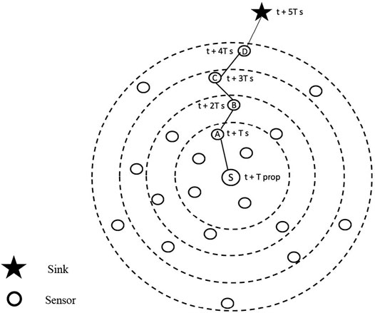
FIGURE 5. The selection of the path for node S at time t.

FIGURE 6

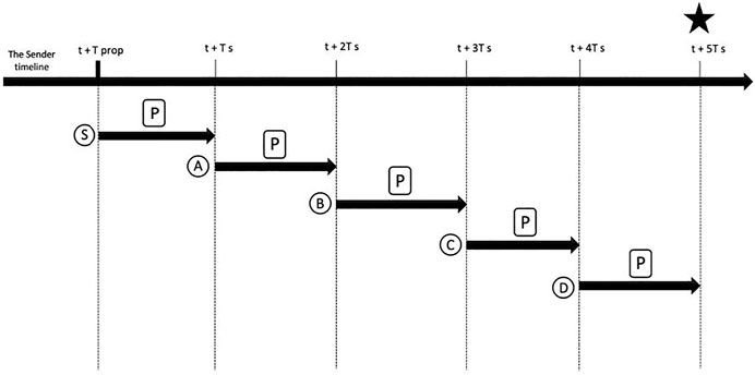
FIGURE 6. Timeline for Figure 5.

Best Path Selection Criteria

In order to extend the lifetime of UASNs, the appropriate best path selection criteria should be carefully chosen. Indeed, selecting the path with the least number of hops consumes less overall energy as the number of intermediate sensors is reduced but may lead to the exhaustion of some sensor batteries if they are extensively used. Therefore, taking into account the remaining energy budget of sensors along the path is crucial in order to increase the network lifetime. That is why our main criterion to select the best energy-efficient path is the highest minimum remaining energy. Accordingly, once all the paths are established, MPODF will check the remaining energy for every node in every path in order to determine the node’s minimum remaining energy for every possible path. The path with the highest node’s minimum remaining energy will be selected even if it is a longer path. If multiple paths with the highest minimum remaining energy are found, then the path with the highest average remaining energy will be selected. The average remaining energy is determined by summing all the remaining energies of the nodes along a path and then dividing by the total number of involved nodes in the path. If the last criterion is still satisfied by many paths, in this case, MPODF chooses the path with the least number of hops as the best one in order to break the tie. Figure 7 illustrates the process of selecting the best path to the sink in the MPODF protocol.

FIGURE 7

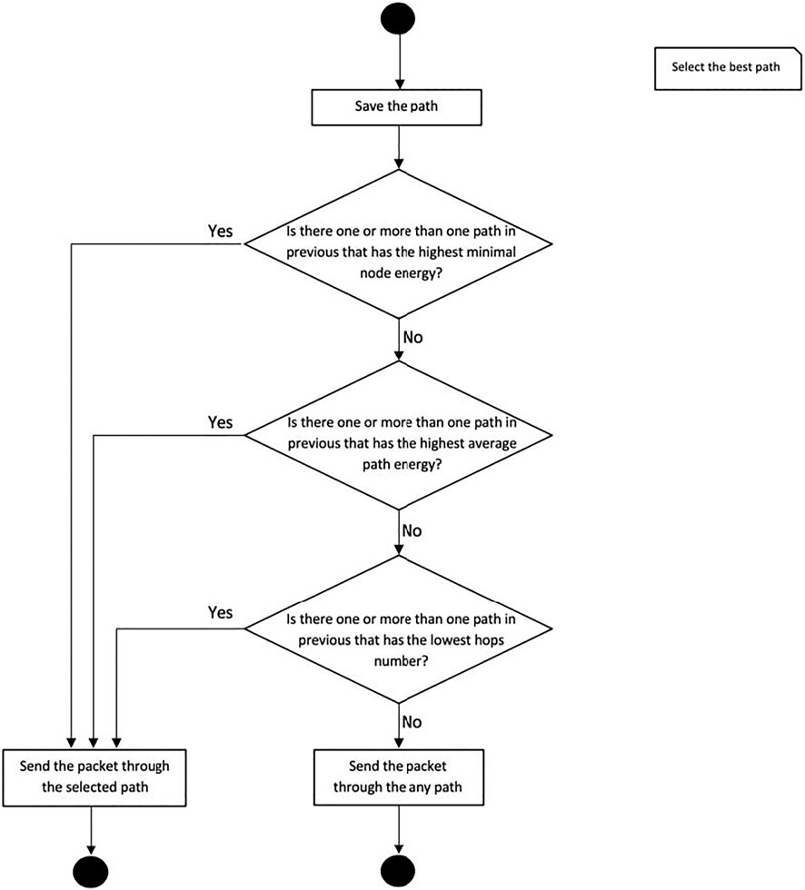
FIGURE 7. The process of selecting the optimal path in an MPODF protocol.

Performance Evaluation

This article is dedicated to evaluating the performance of MPODF and to assess its energy efficiency in a highly dynamic network topology. To do so, various performance metrics will be evaluated, namely, the packets’ delivery ratio, the undelivered packets’ ratio, the end-to-end delay, the average consumed energy per node, the average number of hops of selected paths toward the sink, and the average consumed energy per bit. Moreover, in order to assess the performance of our protocol, we are evaluating it under different mobility scenarios with varying water current velocities, namely, 1 m/s, 3 m/s, and 5 m/s. Furthermore, we compare MPODF with the flooding protocol in order to assess the energy efficiency of prediction-based protocols. Note that the flooding protocol is still one of the most efficient routing protocols in highly dynamic 3D networks. Results show that MPODF outperforms the flooding routing protocol in terms of energy conservation per node as well as per successful bit.

Overview About the Result Analysis Process

In order to meticulously and exclusively assess the performance of our routing protocol, MPODF, we use 400 sensor nodes randomly scattered in a freely floating underwater domain. The used mobility model has many parameters that depend on the underwater environment. Indeed, considering sea, lake, or river will impact the value of the used parameters. In our case, our simulation results are valid for any shallow water with a bidirectional current mobility. Moreover, it is worth pointing out that any change in underwater environment characteristics such as salinity, tide, and bathymetry will first impact the mobility model parameters, and hence, the data communication will be impacted since it highly depends on the used mobility model. One freely floating sink is responsible for collecting the data from sensor nodes. In order to run our mobility prediction module as explained in Paper III, we assume that the nodes’ initial positions are known.

In MPODF, the time is slotted. The slot duration equals $T_s=T_{propagation}+T_{transmission}$. The slot duration is simply the needed time for a data packet to arrive at the next forwarder neighbor.

Table 3 summarizes the simulation parameters.

TABLE 3

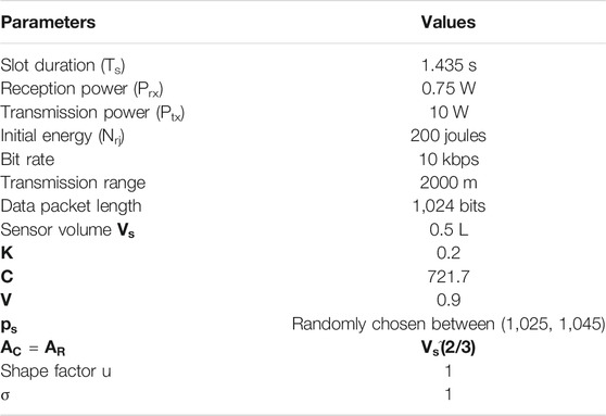
TABLE 3. General simulation parameters.

It is worth pointing out that in addition to the comparison with the flooding protocol, we assess the performance of MPDOF under different mobility conditions. Indeed, high-speed water current results in a great and fast change in the location of nodes, and hence, the topology of UASNs changes frequently. Therefore, the impact of water currents on the data forwarding algorithms needs to be analyzed. In our simulations, we evaluate the impact of three different water current velocities on our protocol, namely, 1 m/s, 3 m/s, and 5 m/s. Intuitively, the mobility speed influences the network performance metrics in UWASNs. In fact, a higher mobility speed implies two main effects: i) nodes experience more meetings on average and ii) meetings tend to have a shorter duration.

Our target in the experiment is to assess the MPDOF performance in terms of the packet delivery ratio, undelivered packet ratio, energy per node, energy per bit, end-to-end delay, and average number of hops toward the sink. The next sections are devoted to assessing the performance of our MPDOF under three different mobility scenarios.

Evaluation of the MPODF Protocol

Packet Delivery Ratio

The packet delivery ratio refers to the total number of successfully received packets by the sink during the simulation time. Recall that three mobility scenarios with three different water current velocities are considered, namely, 1 m/s, 3 m/s, and 5 m/s. Figure 8 depicts the network delivery ratio for the three mobility scenarios as a function of the traffic rate. First, Figure 8 shows that the network throughput increases with the traffic rate. In fact, the higher the traffic generation rate, the more packets will be delivered to the sink node. Most importantly, the first mobility with a water speed of 1 m per second has an overall higher data packet delivery ratio compared to the other two mobility scenarios. Indeed, as expected, the lower the water speed, the higher the packet delivery ratio. In fact, for low values of the water current speed, the whole network topology is slowly varying, and hence, even farther nodes will be able to successfully deliver their data packets as the network is almost static, as opposed to highly dynamic networks, where only nodes closer to the sink will succeed in delivering their packets, and hence, the network delivery ratio will decrease as most of the packets will be undelivered as they come from far nodes.

FIGURE 8

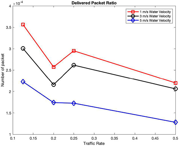
FIGURE 8. The delivered packet ratio simulation result.

Undelivered Packet Ratio

The undelivered packet ratio refers to the ratio of packets that cannot be delivered to the sink by all nodes during the simulation time due to the inability to find a path to the sink.

Figure 9 depicts the undelivered packet ratio with respect to the three mobility scenarios. Note that, according to our protocol, MPDOF, packets are considered undelivered if no path was found to the sink after ten hops. Indeed, the time-to-live (TTL) field in MPDOF packets is set to 10. Accordingly, if no path to the sink was found after ten rounds, then the packet is rejected, and the packet delivery is withdrawn. Indeed, MPODF is a prediction-based routing protocol where a path to the sink needs to be set before proceeding to send the packet. If the prediction module fails to find a path, the packet delivery will be withdrawn, and the packet is considered undelivered. In other words, using the mobility model, MPODF predicts potential paths to the sink. However, if no path is found, then the packet delivery at that time will be abandoned. According to Figure 9, the higher the network mobility, the higher the ratio of undelivered packets. Indeed, when the water currents’ velocity increases, the sink reachability as well as the network connectivity may be badly affected. In fact, when the network topology dynamically changes, the network is frequently partitioned, and hence, the sink becomes unreachable. To illustrate this frequent partition of the network, Figure 10 shows the time evolution of the size of the largest connected component in the network when the water current velocity equals 5 m/s. Note the fast and frequent fluctuations of the size of the largest connected component as nodes can get closer or farther rapidly due to the network mobility. Consequently, the sink reachability is badly affected which justifies the increase of the packet undelivered ratio with the water current velocity.

FIGURE 9

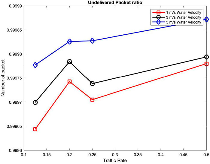
FIGURE 9. The undelivered packet simulation result.

FIGURE 10

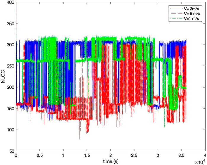
FIGURE 10. The size of the largest connected component with respect to time.

Average Number of Hops

Figure 11 illustrates the average number of hops in a successfully delivered packet as a function of the data generation rate for the three mobility scenarios. First, note that when the network mobility is reduced (1 m/s), the average number of hops toward the sink is higher. Indeed, when the network topology dynamics are rather stable, even the far nodes from the sink will succeed in delivering their data packets. However, when the water current speed increases, only nodes closer to the sink succeed in delivering their packet which justifies the reduction of the average number of hops with the increase of the water velocity. Moreover, note the decrease of the average number of hops with the traffic rate. Indeed, it is absolutely true that as more packets are generated inside the network, the delivery ratio increases as shown in Figure 8, but it will be more restricted to nodes closer to the sink. In fact, when the traffic generation rate increases, nodes closer to the sink will succeed in delivering much more packets which will increase the packet delivery ratio and decrease the average number of hops toward the sink for the successfully received packets.

FIGURE 11

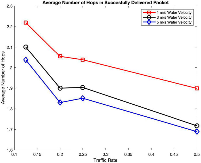
FIGURE 11. The average number of hops.

End-to-End Delay

Figure 12 demonstrates the end-to-end delay as a function of the data generation rate for MPODF under the three mobility scenarios. The end-to-end delay is computed as the amount of time from the packet generation until the successful reception by the sink. Note that, as expected, the end-to-end delay is perfectly proportional to the average number of hops. Indeed, the end-to-end delay can be simply expressed as follows:

$T_{end-to-end}=N_{av-hop}\times T_s,$

where $N_{av-hop}$ denotes the average number of hops. Consequently, the end-to-end delay behavior as a function of the traffic rate and under the three mobility scenarios is easily explained by the behavior of the average number of hops which was explained in Average Number of Hops.

FIGURE 12

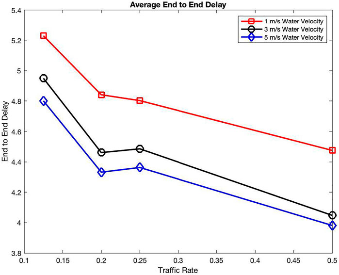
FIGURE 12. The average end-to-end delay.

Energy per Node

Figure 13 shows the average consumed energy per node for the three mobility scenarios. The energy per node is the average consumed energy by a sensor node during the network lifetime. The average energy consumption per node increases with the traffic rate. Indeed, the higher the packet generation rate, the more the energy will be consumed by the network nodes, trying to forward the packets to the sink. In the dynamic environment, our protocol is highly affected by the water velocity in terms of the consumed energy.

FIGURE 13

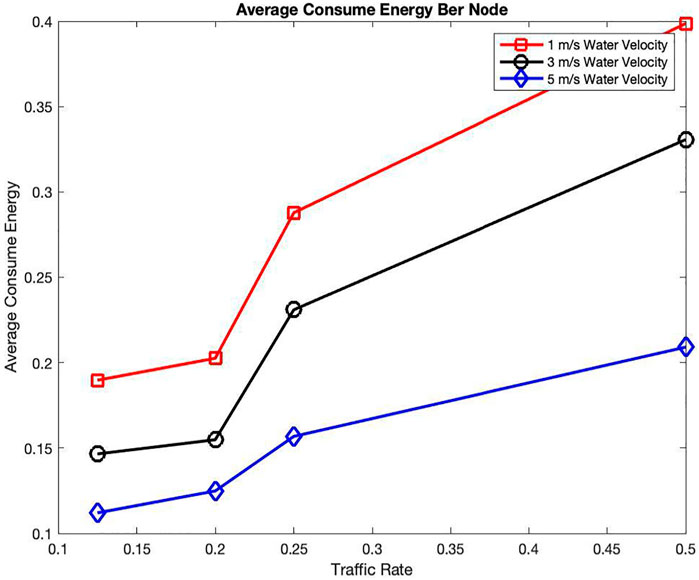
FIGURE 13. The consumed energy per node.

Most importantly, the node’s average energy consumption is high when the network mobility is limited. Indeed, the highest energy consumption is achieved with the lowest water velocity since the packet delivery ratio is the highest. In fact, it is shown in Figure 8 that the packet delivery ratio increases when the water velocity decreases since the network mobility is limited. This increase in the packet delivery ratio will automatically increase the node’s energy consumption since much more packets are delivered to the sink.

Energy per Bit

Figure 14 shows the average consumed energy per bit for our protocol under the three mobility scenarios. The energy per bit is the total consumed energy by all the nodes during the network lifetime divided by the total number of successfully received data packets. It is worth pointing out that the average consumed energy per bit increases when the water velocity decreases. Recall that, according to Figures 8, 11, when the network mobility is reduced, the packet delivery ratio and the average consumed energy per node increase which will increase the energy per bit. Consequently, as the network topology slowly varies, more data packets are delivered to the sink, and hence, the energy per bit increases.

FIGURE 14

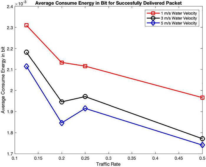
FIGURE 14. The consumed energy per bit.

Moreover, note the decrease of the average consumed energy per bit with the traffic rate. As explained in Figures 8, 9, when the traffic generation rate increases, the packet delivery ratio increases, and the average number of hops decreases. Consequently, more packets are delivered through the shortest paths. Therefore, the average consumed energy per bit will decrease resulting in a better energy efficiency of the network.

Comparison of Mobility Prediction Optimal Data Forwarding to the Flooding Protocol

We compare the performance of our protocol with the flooding routing protocol. Flooding is a simple routing technique that requires no network information such as nodes’ positions and no routing overhead to set a path. Indeed, according to the flooding, no extra packets are exchanged among neighbors to set a path toward the sink. Although flooding highly consumes the network resources, especially in terms of link capacity and energy since it uses every possible path in the network, it has its own strength. First, the flooding algorithm is easy to implement. Indeed, in uncontrolled flooding, each node unconditionally distributes packets to each of its neighbors, and hence, no computational overhead is introduced to select a path. Second, the flooding protocol is robust as it guarantees the packet delivery if a path exists which results in a high packet delivery ratio as all the possible paths are used. Note that such a feature is required, especially in highly dynamic 3D networks, where the main objective is to find a path toward the sink. Finally, the flooding protocol by design does not require any network information to be shared by nodes, neither topological nor neighborhood information. Figure 15 illustrates the functioning of the flooding protocol.

FIGURE 15

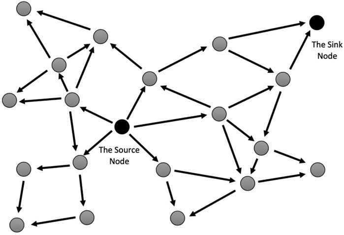
FIGURE 15. The flooding routing protocol.

Energy efficiency in underwater networks is essential as nodes are often operated by batteries and their supply is difficult to replenish. Furthermore, considering that UASNs are influenced by atmospheric environmental factors contributing to unpredictable network dynamics, a high probability of error, and large propagation delays, it is much more important to examine the energy efficiency of our proposed MPODF protocol. To do so, we will compare the energy efficiency of our protocol with the flooding algorithm in terms of energy per node and energy per bit. Recall that the flooding protocol is the most robust solution in highly dynamic networks that is why it is chosen as a reference protocol for comparison purposes. In fact, the flooding protocol benefits from a higher node speed and delivers more packets successfully to their destinations more quickly, compared to the case of slower node movements. Therefore, the flooding takes advantage from increased node mobility in terms of average end-to-end delivery delay and a packet delivery ratio as frequent node meetings contribute to quicker and more packet delivery to the final destination. However, the flooding protocol does not control how conveniently the packets are replicated; hence, its energy efficiency is questionable.

Energy per Node

Figure 16 illustrates the average energy consumption per node as a function of the traffic rate for the three mobility scenarios of our MPODF protocol along with the flooding. Most importantly, the flooding protocol achieves by far higher average energy consumption per node compared to MPODF due to the greedy flooding algorithm which involves all possible nodes for each forwarding hop. Consequently, the higher the traffic rate, the higher the delivered packet ratio and hence the higher the consumed energy per node.

FIGURE 16

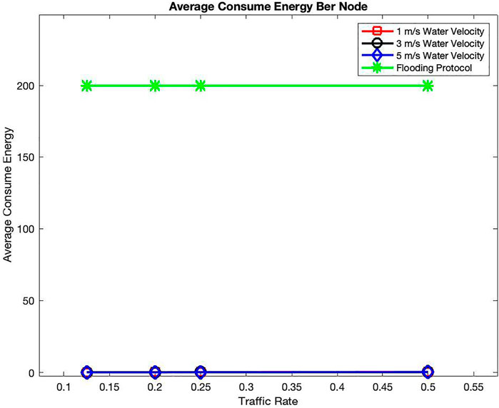
FIGURE 16. The consumed energy per node of the flooding protocol.

Energy per Bit

Figure 17 shows the average consumed energy per successful bit for the three mobility scenarios of our MPODF protocol along with the flooding. Most importantly, the flooding routing protocol has the highest consumed energy per bit since it achieves the highest node energy consumption (as shown in Figure 16). Indeed, the flooding uses all the possible paths toward the sink for each generated packet. Hence, the nodes drain their energy budget quickly resulting in nonreachable sink which highly increase the energy cost of every successfully delivered bit to the sink.

FIGURE 17

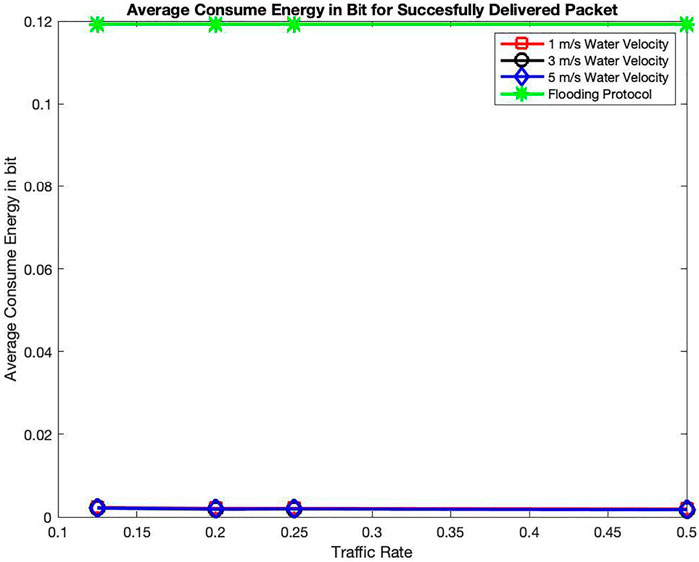
FIGURE 17. The consumed energy per bit of the flooding protocol.

Conclusion

In this article, we evaluated our data forwarding protocol, MPODF, which aims at maximizing the network lifetime by selecting the optimal energy-efficient path to the sink based on the residual energy of sensor nodes. Most importantly, we showed that our protocol performs better in terms of energy efficiency and delivery ratio when the network topology is slowly varying as the network tends to be more stable. As for the end-to-end delay, when the network mobility is reduced, it increases since farther nodes succeed in delivering their data packets, as opposed to highly dynamic networks, where the delivery is restricted to nodes closer to the sink which will reduce the end-to-end delay. Moreover, it is worth pointing out that our MPDOF protocol with different water velocity mobility scenarios outperforms the flooding in terms of energy conservation. As a future work, an experimental evaluation will be conducted in a real testbed to assess the performance of MPODF in a real environment. Furthermore, more underwater scenarios with different characteristics will be evaluated to assess the performance of MPODF in various underwater environments.

Data Availability Statement

The original contributions presented in the study are included in the article/Supplementary Material, and further inquiries can be directed to the corresponding author.

Author Contributions

FB has conceived the research study. GA has implemented the research work and obtained the results shown here. The two authors have analyzed and discussed the results and written the manuscript.

Conflict of Interest

The authors declare that the research was conducted in the absence of any commercial or financial relationships that could be construed as a potential conflict of interest.

Publisher’s Note

All claims expressed in this article are solely those of the authors and do not necessarily represent those of their affiliated organizations, or those of the publisher, the editors and the reviewers. Any product that may be evaluated in this article, or claim that may be made by its manufacturer, is not guaranteed or endorsed by the publisher.

References

Ahmed, M., Salleh, M., and Channa, M. I. (2017). Routing Protocols Based on Node Mobility for Underwater Wireless Sensor Network (UWSN): A Survey. J. Netw. Comput. Appl. 78, 242–252. doi:10.1016/j.jnca.2016.10.022

CrossRef Full Text | Google Scholar

Ayaz, M., Abdullah, A., and Faye, I. (2010). “Hop-by-hop Reliable Data Deliveries for Underwater Wireless Sensor Networks,” in Proceedings of the 2010 International Conference on Broadband, Wireless Computing, Communication and Applications (BWCCA) (Fukuoka, Japan), 363–368.

Google Scholar

Ayaz, M., and Abdullah, A. (2009). “Hop-by-hop Dynamic Addressing Based (H2-DAB) Routing Protocol for Underwater Wireless Sensor Networks,” in Proceedings of the International Conference on Information and Multimedia Technology (ICIMT’09) (Jeju Island, Korea, 436–441.

Google Scholar

Baccour, N., Koubâa, A., Youssef, H., Ben Jamâa, M., do Rosário, D., Alves, M., and Becker, L. B. (2010). “F-LQE: A Fuzzy Link Quality Estimator for Wireless Sensor Networks,” in Proceedings of the European Conference on Wireless Sensor Networks (Portugal: Coimbra), 240–255. doi:10.1007/978-3-642-11917-0_16

CrossRef Full Text | Google Scholar

Bouabdallah, F. (2019). Time Evolution of Underwater Sensor Networks Coverage and Connectivity Using Physically Based Mobility Model. Wireless Commun. Mobile Comput. 2019, 1–9. doi:10.1155/2019/9818931

CrossRef Full Text | Google Scholar

Chen, Y.-S., and Lin, Y.-W. (2013). Mobicast Routing Protocol for Underwater Sensor Networks. IEEE Sensors J. 13 (2), 737–749. doi:10.1109/JSEN.2012.2226877

CrossRef Full Text | Google Scholar

Coutinho, R. W. L., Boukerche, A., Vieira, L. F. M., and Loureiro, A. A. F. (2016). Geographic and Opportunistic Routing for Underwater Sensor Networks. IEEE Trans. Comput. 65 (2), 548–561. doi:10.1109/TC.2015.2423677

CrossRef Full Text | Google Scholar

Coutinho, R. W. L., Boukerche, A., Vieira, L. F. M., and Loureiro, A. A. F. (2018). Underwater Wireless Sensor Networks. ACM Comput. Surv. 51 (1), 1–36. doi:10.1145/3154834

CrossRef Full Text | Google Scholar

Dhurandher, S. K., Borah, S. J., Woungang, I., Bansal, A., and Gupta, A. (2018). A Location Prediction-Based Routing Scheme for Opportunistic Networks in an IoT Scenario. J. Parallel Distributed Comput. 118, 369–378. doi:10.1016/j.jpdc.2017.08.008

CrossRef Full Text | Google Scholar

Han, G., Long, X., Zhu, C., Guizani, M., Bi, Y., and Zhang, W. (2019). An AUV Location Prediction-Based Data Collection Scheme for Underwater Wireless Sensor Networks. IEEE Trans. Veh. Technol. 68 (6), 6037–6049. doi:10.1109/TVT.2019.2911694

CrossRef Full Text | Google Scholar

Hu, T., and Fei, Y. (2013). “An Adaptive Routing Protocol Based on Connectivity Prediction for Underwater Disruption Tolerant Networks,” in IEEE Global Communications Conference (Atlanta, GA: GLOBECOM) 2013, 65–71.

Google Scholar

Hwang, D., and Kim, D. D. F. R. (2008). “Directional Flooding-Based Routing Protocol for Underwater Sensor Networks,” in Proceedings of the 2008 IEEE OCEANS (Quebec, QC, Canada), 1–7.

Google Scholar

Ibrahim, D. M., Eltobely, T. E., Fahmy, M. M., and Sallam, E. A. (2014). “. Enhancing the Vector-Based Forwarding Routing Protocol for Underwater Wireless Sensor Networks: A Clustering Approach,” in ICWMC 2014 (Spain: Sevilla), 8.

Jafri, M. R., Ahmed, S., Javaid, N., Ahmad, Z., and Qureshi, R. (2013). Amctd: Adaptive Mobility of Courier Nodes in Threshold- Optimized DBR Protocol for Underwater Wireless Sensor Networks. Proceedings of the 2013 Eighth International Conference on Broadband and Wireless Computing, Communication and Applications (BWCCA). Compiegne, France, 93–99.

Google Scholar

Jafri, M. R., Sandhu, M. M., Latif, K., Khan, Z. A., Yasar, A. U. H., and Javaid, N. (2014). Towards Delay-Sensitive Routing in Underwater Wireless Sensor Networks. Proced. Comput. Sci. 37, 228–235. doi:10.1016/j.procs.2014.08.034

CrossRef Full Text | Google Scholar

Khan, A. H., Jafri, M. R., Javaid, N., Khan, Z. A., Qasim, U., and Imran, M. (2015). DSM: DSM: Dynamic Sink Mobility Equipped DBR for Underwater WSNs. Proced. Comput. Sci. 52, 560–567. doi:10.1016/j.procs.2015.05.036

CrossRef Full Text | Google Scholar

Liu, G., and Li, Z. (2010). “Depth-based Multi-Hop Routing Protocol for Underwater Sensor Network,” in Proceedings of the 2010 2nd International Conference on Industrial Mechatronics and Automation (ICIMA) (Wuhan, China), 268–270.2

Google Scholar

Nicolaou, N., See, A., Xie, P., Cui, J., and Maggiorini, D. (2007). Improving the Robustness of Location-Based Routing for Underwater Sensor Networks. In OCEANS 2007 - Europe, 1–6.

Google Scholar

Noh, Y., Lee, U., Lee, S., Wang, P., Vieira, L. F. M., Cui, J.-H., et al. (2016). HydroCast: Pressure Routing for Underwater Sensor Networks. IEEE Trans. Veh. Technol. 65 (1), 333–347. doi:10.1109/tvt.2015.2395434

CrossRef Full Text | Google Scholar

Nowsheen, N., Karmakar, G., and Kamruzzaman, J. (2014). MPDF: Movement Predicted Data Forwarding Protocol for Underwater Acoustic Sensor Networks. In the 20th Asia-Pacific Conference on Communication (APCC2014). Thailand: Pattaya, 100–105.

Google Scholar

Rahman, R. H., Benson, C., and Frater, M., (2012). Routing Protocols for Underwater Ad Hoc Networks In 2012 Oceans - Yeosu, Yeosu, Korea (South), pp. 1–7. doi:10.1109/OCEANS-Yeosu.2012.6263636

CrossRef Full Text | Google Scholar

Tian, Q., Wen, J., and Yu, G. (2010). “Space-Time-Energy Based Forwarding Protocol for Underwater Acoustic Sensor Networks,” in 2010 International Conference on Communications, Circuits and Systems (ICCCAS). Chengdu, China, 98–102. doi:10.1109/ICCCAS.2010.5582041

CrossRef Full Text | Google Scholar

Umar, A., Javaid, N., Ahmad, A., Khan, Z., Qasim, U., Alrajeh, N., et al. (2015). DEADS: Depth and Energy Aware Dominating Set Based Algorithm for Cooperative Routing along with Sink Mobility in Underwater WSNs. Sensors 15 (6), 14458–14486. doi:10.3390/s150614458

PubMed Abstract | CrossRef Full Text | Google Scholar

Wahid, A., and Kim, D. (2012). An Energy Efficient Localization-free Routing Protocol for Underwater Wireless Sensor Networks. Int. J. Distributed Sensor Networks 8 (4), 307246. doi:10.1155/2012/307246

CrossRef Full Text | Google Scholar

Wahid, A., Lee, S., Kim, D., and Lim, K.-S. (2014). MRP: A Localization-free Multi-Layered Routing Protocol for Underwater Wireless Sensor Networks. Wireless Pers Commun. 77 (4), 2997–3012. doi:10.1007/s11277-014-1690-6

CrossRef Full Text | Google Scholar

Wang, A., Li, B., and Zhang, Y., (2018). Underwater Acoustic Channels Characterization for Underwater Cognitive Acoustic Networks in 2018 International Conference on Intelligent Transportation, Big Data & Smart City (ICITBS), Xiamen, China, pp. 223–226. doi:10.1109/ICITBS.2018.00065

CrossRef Full Text | Google Scholar

Wei, B., Luo, Y.-m., Jin, Z., Wei, J., and Su, Y. (2013). “ES-VBF: An Energy Saving Routing Protocol,” in Proceedings of the 2012 International Conference on Information Technology and Software Engineering. Editors W. Lu, G. Cai, W. Liu, and W. Xing (Berlin, Heidelberg: Springer Berlin Heidelberg), vol. 210, 87–97. doi:10.1007/978-3-642-34528-9_10

CrossRef Full Text | Google Scholar

Xie, P., Cui, J.-H., and Lao, L. (2006). “VBF: Vector-Based Forwarding Protocol for Underwater Sensor Networks,” in NETWORKING 2006. Networking Technologies, Services, and Protocols; Performance of Computer and Communication Networks; Mobile and Wireless Communications Systems. Editors F. Boavida, T. Plagemann, B. Stiller, C. Westphal, and E. Monteiro (Berlin, Heidelberg: Springer Berlin Heidelberg), 3976, 1216–1221. doi:10.1007/11753810_111

CrossRef Full Text | Google Scholar

Xie, P., Zhou, Z., Peng, Z., Cui, J.-H., and Shi, Z. (2009). “Void Avoidance in Three-Dimensional mobile Underwater Sensor Networks,” in Proceedings of the International Conference on Wireless Algorithms, Systems, and Applications (Boston, MA, USA), 305–314. doi:10.1007/978-3-642-03417-6_30

CrossRef Full Text | Google Scholar

Yan, H., Shi, Z. J., and Cui, J.-H. (2008). “DBR: Depth-Based Routing for Underwater Sensor Networks,” in NETWORKING 2008 Ad Hoc and Sensor Networks, Wireless Networks, Next Generation Internet. NETWORKING 2008. Lecture Notes in Computer Science. Editors A. Das, H. K. Pung, F. B. S. Lee, and L. W. C. Wong (Berlin, Heidelberg: Springer), 4982, 15.

Zhang, Z., Lin, S.-L., and Sung, K.-T. (2010). “A Prediction-Based Delay-Tolerant Protocol for Underwater Wireless Sensor Networks,” in International Conference on Wireless Communications & Signal Processing (WCSP) (Suzhou, China), 1–6. doi:10.1109/WCSP.2010.5633659

CrossRef Full Text | Google Scholar

Zorzi, M., Casari, P., Baldo, N., and Harris, A. (2008). Energy-Efficient Routing Schemes for Underwater Acoustic Networks. IEEE J. Select. Areas Commun. 26 (9), 1754–1766. doi:10.1109/JSAC.2008.081214

CrossRef Full Text | Google Scholar