Data mining for prediction and interpretation of bacterial population behavior in food

1 Introduction

Different types of microorganisms are present in food. Some of these cause foodborne illness and food spoilage. To control food pathogens and spoilage bacteria, various preservation techniques have been developed to prevent harmful bacteria from growing during processing, distribution, and storage. Many factors influence the microbial response in food ecosystems. For instance, temperature, pH, water activity (a_w), antimicrobial additives, and gas components can affect bacterial population behavior (Leistner, 2000; Doyle et al., 2019), even though the effects on bacterial growth and inactivation vary by bacterial species or genus. Adjusting the various environmental conditions in food enables the suppression of bacterial growth and food spoilage (Gould, 1996; Leistner, 2000). Thus, appropriate microbiological control can help prevent food loss and improve food safety.

To quantify and evaluate bacterial growth for control, many studies on microbiological response in food have been conducted since Roberts & Jarvis (1983) introduced predictive microbiology, which originated from the research by Bigelow (1921), Bigelow & Esty (1920), and Esty & Meyer (1922). Each experimental data on bacterial growth and inactivation was obtained by counting the number of colonies on the culture plate as viable cell counts or by measuring optical density for the cell density over time under controlled conditions, such as temperature, pH, and a_w. Microbial responses in food have been explained by mathematical models, the main exploratory variables of which are temperature, pH, and a_w (Ross and McMeekin, 1994; Jagannath and Tsuchido, 2003). Over the last 40 years, experimental data on microbial responses to the food environment have been collected by research institutions, universities, and companies according to their objectives. The accumulated data are stored in databases such as the ComBase database (www.combase.cc), which was developed to provide easy access to microbiological data in research establishments and publications produced by different laboratories (Baranyi et al., 2004). Currently, every effort is vital for collecting data with similar species or conditions through literature or database to assess product safety. A comprehensive statistical analysis is needed for understanding bacterial population behavior regardless of food and bacteria.

Studies have been conducted to understand the global trends of microbial responses from the accumulated data. In predictive microbiology, studies have used meta-analysis, which is a method to amalgamate, summarize, or review previous quantitative research for identifying trends with a statistical model of specific foods and bacteria [e.g., evaluating inactivation of Escherichia coli in fermented meat (McQuestin et al., 2009), meta-analysis for quantitative microbiological risk assessments and benchmarking data (den Besten and Zwietering, 2012), growth and inactivation of Listeria monocytogenes in milk or non-thermal inactivation of Listeria monocytogenes in fermented sausages (Mataragas et al., 2015)]. Statistical models generally require analysts to specify the functional form between explanatory variables and response variables (Hochachka et al., 2007). Studies using meta-analysis have provided results that suit some objectives, such as trends in maximum growth rate or bacterial growth/inactivation by foods. However, a meta-analysis with statistical models alone is not necessarily systematic and tends to be fragmentary in terms of cross-food/bacteria analysis. Bacterial growth is affected by not only factors such as temperature, pH, and a_w, but also cell density (Koutsoumanis and Sofos, 2005; Skandamis et al., 2007; Bidlas et al., 2008), characteristics of each food, and gaseous atmosphere (Doyle et al., 2019). Identifying complex relationships between food and bacteria requires the development of complex mathematical formulas with high-dimensional variables. To predict the bacterial population change and to explore the influence of each factor on microbial response using big data, a non-parametric approach, which needs to develop no hypothesis based on domain knowledge, is considered useful (Deringer et al., 2021).

Data mining is an effective method for analyzing large amounts of accumulated data. Data mining is the secondary analysis of a large database to identify and interpret hidden patterns (Hand, 1998). The recent accumulation of big data has promoted the development of databases in various fields. Consequently, data mining has been employed in many fields such as agriculture (Cortez et al., 2009; Gulyaeva et al., 2020), ecology (Hochachka et al., 2007; Ross et al., 2018), healthcare and medicine (Cios and William Moore, 2002; Delen et al., 2005; Koh and Tan, 2005; Mohanty et al., 2022), and food quality (Cortez et al., 2009; Jiménez-Carvelo et al., 2019; Nychas et al., 2021). Using machine learning, the relationship between the response and function can be determined empirically from the data. This approach can discover new knowledge of these patterns. To the best of our knowledge, only one data mining study has been conducted in the field of predicting bacterial population behavior. Hiura et al. (2021) predicted the bacterial behavior of Listeria monocytogenes using the ComBase database of microbial responses to food environments. The ComBase database contains information about bacteria and foods, such as the name of the bacterial genus or species and the category or name of the medium or food. Such information enables us to extract the comprehensive characteristics of bacterial responses, such as the association between food ecosystems and bacterial population changes, by analyzing the data reported in previous studies. In this manner, exploring the whole trend of interactions between microbial growth and inactivation and conditions from accumulated data would have an advantage in the comparison and evaluation of bacterial population changes in various bacteria and different foods.

In the present study, the objective was to not only develop a single machine learning model for predicting population behavior of food-related bacteria in various kinds of food, but to also visualize the effect of pH, a_w, and temperature using a data mining approach. Data regarding the change in viable cell number over time were used for eight foodborne and food spoilage bacteria: “Aeromonas hydrophila,” “Bacillus cereus,” “Escherichia coli,” “Listeria monocytogenes,” “Pseudomonas spp.,” “Staphylococcus aureus,” “Salmonella spp.,” and “Yersinia enterocolitica.” The microbial responses to the food environment were collected from the ComBase database. The collected data included population behavior based on 15 food categories —“beef,” “culture medium,” “pork,” “poultry,” “seafood/fish,” “vegetable or fruit and their products,” “water,” “dessert food,” “milk,” “sausage,” “cheese,” “eggs and egg product,” “juice and beverage,” “sauce/dressing,” and “bread”— with temperature ranging 0°C–25°C. Data mining and machine learning approaches provide information concerning population behavior and its effects on food ecosystems.

2 Materials and methods

2.1 Data selection from ComBase database

The ComBase database contains quantified microbial responses to food with approximately 60,000 records collected from various research establishments and publications. Changes in the bacterial density over time were recorded for each experimental condition. The dataset of a change in bacterial density over time in ComBase contains “Record ID,” “Organism,” “Food category,” “Food name,” “Temperature,” “pH,” “a_w,” “Conditions,” “Time,” and “Viable cell counts”. Each dataset of changes in a bacterial population is assigned a “Record ID,” which allows us to recognize one series of experiments on population behavior.

In this study, we investigated changes in the populations of eight pathogenic and food spoilage bacteria: A. hydrophila, B. cereus, E. coli, L. monocytogenes, Pseudomonas spp. (Pseudomonads), S. aureus, Salmonella spp. (Salmonella), and Y. enterocolitica. These bacteria are known to cause food spoilage and foodborne illnesses. Fifteen kinds of food categories were included “beef,” “culture medium,” “pork,” “poultry,” “seafood/fish,” “vegetable or fruit and their products,” “water,” “dessert food,” “milk,” “sausage,” “cheese,” “eggs and egg product,” “juice and beverage,” “sauce/dressing,” and “bread.” The data used for model development and evaluation were those with temperatures ranging from 0°C to 25°C and containing greater than or equal to four observed values in each series of experiments on bacterial population behavior. In addition, records for which viable counts at 0 h were unavailable were excluded, because the objective values, $\mathit{log}{N}_t/N_0$ can not be calculated. Records containing preservatives such as acetic acid, lactic acid, nitrite, and sorbic acid were also excluded. In total, 9,091 records of bacterial population behavior were extracted from ComBase and 101,861 viable count data were used. Table 1 summarizes the data selected for this study. The entire “Record ID” list extracted from ComBase is available online in Supplementary Data S1.

TABLE 1

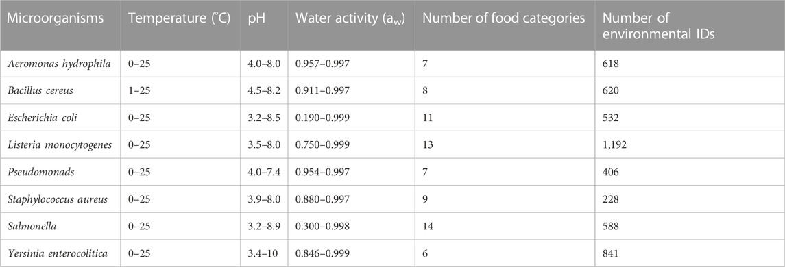
TABLE 1. Summary of the extracted data from ComBase.

2.2 Data preprocessing

In the present study, we set the change ratio of viable counts as the objective variable to predict bacterial behavior to evaluate both the increase and decrease in the bacterial population. For each Record ID, the cell concentration was transformed to a common logarithm of the change ratio of viable counts to the initial cell number $\mathit{log}{N}_t/N_0$ defined in Eq. 1:

$\log N_t-\log N_0=\log \frac{N_t}{N_0}(1)$

where $\log N_t$ and $\log N_0$ are viable cell concentrations (log colony forming unit (CFU)/g) when the storage time is $t$ (h) and the logarithm of the initial cell concentration (log CFU/g), respectively. We used $\mathit{log}{N}_t/N_0$ as the objective variable. Eight types of explanatory variables were included: “Time (h),” “Temperature (°C),” “pH,” “a_w,” “Initial cell number (log CFU/g),” “Food category,” “Food name,” and “Organism.” The data included both numerical and categorical data. “Time,” “Temperature,” “pH,” ‘a_w,” and “Initial cell number” were numerical data, which were used without modification for model development. The viable cell concentration at 0 h was used as the initial cell number for each record ID. Furthermore, because food category, food name, and organism are categorical variables, they were replaced with dummy variables, which is a common technique in models based on decision trees (Hiura et al., 2021). The 15 food categories were converted as 1–15. The types of food names were converted to 1–261. The eight organisms were converted to 1–8. The data acquired from ComBase included “Record ID” and could be employed for each series of experimental results of pathogen survival registered based on the record ID. In the original dataset, there are some data that Record IDs are different but the experimental conditions (“Temperature,” “pH,” “aw,” “Food category,” “Food name,” and “Organism”) are the same. To unify the experimental condition, we renamed “Record ID” to “Environmental ID, which avoids overlapping with the experimental conditions in the training and test datasets. The record IDs for which temperature, pH, a_w, food category, food name, and organism were the same were regarded as the results of experiments conducted through different repetitions under the same conditions, and the same “Environmental ID” was reassigned as the result of a single experimental condition. Thus, 9,091 record IDs were assigned to 5,025 environmental IDs. In total, 101,861 observed plots were investigated. In the test dataset, the number of environmental conditions used was 542 and the number of observed plots used was 11,106.

2.3 Model development

2.3.1 eXtreme gradient-boosting tree (XGBoost) model

The XGBoost was first proposed by Chen and Guestrin in 2016. XGboost extends the concept of the Gradient Boosting Decision Tree (GBDT). The GBDT is an iterative decision tree that includes multiple decision trees (Friedman, 2001). The GBDT is a tree-based ensemble technique that uses a decision tree as the base model, and gradient boosting trains it sequentially by adding each base model and fixing the errors generated by the previous tree model. The GBDT method has been widely employed in machine learning and data mining studies (Chang et al., 2018; Nguyen et al., 2019; Rodrigo et al., 2021; Shehadeh et al., 2021). XGBoost was used in the present study because it has several advantages in terms of fewer requirements for feature engineering, allowing steps such as handling missing values without specific processing, and variables without normalization and scaling (Wang et al., 2020; Mohanty et al., 2022). The XGBoost models were built using the XGBoost (Version 1.5.0) Python Package (https://xgboost.readthedocs.io/en/latest/python/index.html).

2.3.2 Modeling procedure

We aimed to develop a machine learning model for predicting bacterial responses to various food environments, characterized by controlling factors such as temperature, pH, and a_w. Eight input variables that included five numerical data types—temperature (°C), pH, a_w, time (h), and initial cell number (log CFU/g)—and three categorical data types—food category, food name, and organism—were used to develop a model to predict change ratio of a bacterial population.

There were several steps to divide the imbalanced whole dataset into training and test dataset. First, the whole dataset was separated by “Microorganisms.” Second, the dataset separated by “Microorganisms” was separated by “Food category.” Third, the dataset separated by “Microorganisms” and “Food category” was randomly divided into 9:1 without overlapping with the experimental conditions in the training and test datasets. Thus, the imbalanced dataset was separated into the training and test dataset. The training dataset was used to build a model for predicting bacterial responses to various food environments, while its hyperparameters were optimized. The test dataset was used to evaluate the performance of the tuned model.

Prior to training the predicting model, the hyperparameters of the XGBoost model used in this study were determined by a 5-fold cross-validation and grid search. Cross-validation validates the model performance using only the training dataset under an arbitrary hyperparameter set. It attempts to avoid overfitting which deteriorates the performance on unknown data (i.e., test dataset). In this method, the training dataset was divided into 5-fold (4-fold of training data and 1-fold of validation data) and then the training data was used to train a model, and validation data was used to verify the performance. Repeating this validation cycle by swapping the validation data with the training data, the performance of the model was validated. A grid search was conducted by selecting each hyperparameter value from a pre-defined range, and thus the highest performing (i.e., optimal) hyperparameters are determined. The XGBoost model hyperparameters were set in some ranges (Supplementary Table S1) and optimized as follows: a maximum tree depth of 9, min_child_weight of 1, gamma of 0.3, subsample of 0.6, colsample_bytree of 0.6, and reg_alpha of 100.

2.4 Evaluation of model accuracy

The prediction accuracy of the developed model was evaluated using 542 test datasets of environmental ID that were not used in model development. The coefficient of determination (R²) and root mean square error (RMSE) were calculated for all test data, each organism, and each food category, as an index to evaluate the accuracy of the model. The R² and RMSE values are given by Eqs 2, 3, respectively:

$R^2=1-\frac{{\sum }_{i=1}^n{\left(y_i-{\widehat{y}}_i\right)}^2}{{\sum }_{i=1}^n{\left(y_i-{\mu }_y\right)}^2}(2)$

$RMSE=\sqrt{\frac{1}{n}{\displaystyle \sum }_{i=1}^n{\left(y_i-{\widehat{y}}_i\right)}^2}(3)$

where $y_i$, ${\widehat{y}}_i$, and ${\mu }_y$ are the $i$ th observed $\mathit{log}{N}_t/N_0$, the $i$ th predicted $\mathit{log}{N}_t/N_0$, and the average observed $\mathit{log}{N}_t/N_0$, respectively. Each evaluation metric was calculated using the Scikit-learn (version 1.0.1) Python package.

2.5 Two-dimensional (2D) plot visualization of bacterial behaviors

Using the developed model, the $\mathit{log}{N}_t/N_0$ was predicted at various pH, a_w, and temperatures when the initial cell count was 4 log CFU/g at 10 days in broth. To visualize microbial response to various environments, the $\mathit{log}{N}_t/N_0$ at 10 days was divided into four levels, “strongly increased” (change > 3-log cycle), “increased” (change of 2 ± 1 log cycle), “survival” (change of 0 ± 1 log cycle), and “decreased” (change of −2 ± 1 log cycle). We then plotted the responses as 2D color maps, to obtain three types of maps, pH–a_w, pH–temperature, and temperature–a_w. To confirm the validity of this 2D plot, we predicted the $\mathit{log}{N}_t/N_0$ and visualized it under some experimental conditions reported in previous studies.

We then compared our 2D color map with the data in the literature on growth/no-growth experiments, which was not recorded in ComBase. The data used for external validation were selected, considering that the experimental conditions are simple enough to describe bacterial behavior by eight explanatory variables. As a representative inactivation process, we cite a study of growth/no growth experiments of L. monocytogenes in broth (Koutsoumanis et al., 2004). The growth/no-growth L. monocytogenes were experimentally observed in a culture medium after 30 days at 25 °C (a), with pH 5.47–5.58 (b) and a_w of 0.965–0.967 (c) after 30 days.

2.6 Interpretation of machine learning model

2.6.1 Feature importance

The feature importance was calculated to interpret the developed model from the process of model development. This allowed us to understand how each explanatory variable contributed to the predicted performance during the training of the XGBoost algorithm. The importance of the features was evaluated using gain, which is an index that shows the usefulness of a feature in constructing a tree-based model. A higher value indicates that the feature significantly affects the predicted $\mathit{log}{N}_t/N_0$. Feature importance was calculated using the XGBoost Python package (https://xgboost.readthedocs.io/en/latest/python/python_api.html).

2.6.2 SHapley Additive eXplanations (SHAP) value

As another approach for model interpretation, we used the SHAP framework proposed by Lundberg and Lee (2017). SHAP is a new and flexible method that addresses the machine learning system as a so-called “black-box model” by providing an interpretation of how strongly the features affect the predicted outcome. Although the feature importance employed by XGBoost is positioned as the global explanation of the model, SHAP can directly measure a local feature explanation for a single sample, which could otherwise go unnoticed (Moncada-Torres et al., 2021). Because SHAP approaches are model-agnostic, they are used with various model types and in many fields of study (Lundberg and Lee, 2017; Agius et al., 2020; Mangalathu et al., 2020; Ndraha et al., 2021; Rodrigo et al., 2021; Yang and Liu, 2021; Zoabi et al., 2021).

The SHAP value for a single feature within a single sample describes the extent to which that feature contributes to the predicted output. A higher SHAP value indicates that a feature has a larger impact on the predicted $\mathit{log}{N}_t/N_0$, whereas a lower SHAP value indicates a smaller impact. A positive SHAP value indicates that a feature makes a positive contribution to the predicted $\mathit{log}{N}_t/N_0$, whereas a negative value indicates a negative contribution. By computing a SHAP value for each data point, a more detailed explanation of the global feature importance, such as the relationship between the feature and its corresponding effect on the output [e.g., SHAP dependence plot (Lundberg et al., 2018)], can be obtained.

SHAP values were calculated using TreeSHAP (Lundberg et al., 2018), and a variant of SHAP, which was developed for tree-based machine learning models, such as XGBoost, as incorporated in the SHAP (Version 0.40.0) Python Package (https://shap.readthedocs.io/en/latest/index.html). All pre-processing steps, model development, and statistical analyses were performed using Python (version 3. 8. 12).

3 Results

3.1 Evaluation of model accuracy

By developing a single machine learning model, our data-mining approach meets in rough agreement with respect to prediction accuracy under various types of microorganisms and food categories. Figure 1 represents overall predicted results including all types of microorganisms and food categories, in which the R² and RMSE values obtained were 0.76 and 1.23, respectively. The accuracy evaluated is consistently convincing compared with that of Hiura et al. (2021) (0.75 for R² and 1.02 for RMSE, respectively). Followed by this, results divided by each microorganism, and by each food category are shown in Figures 2, 3, respectively. For each organism in Figure 2, the RMSE values were 1.35, 1.41, 1.42, 1.20, 1.42, 1.03, 1.07, and 1.08, for A. hydrophila, B. cereus, E. coli, L. monocytogenes, Pseudomonads, S. aureus, Salmonella, and Y. enterocolitica, respectively. In Figure 3, the RMSE values for the culture medium, beef, pork, poultry, sausage, eggs, seafood, milk, cheese, vegetables or fruits, bread, dessert food, beverage, water, and sauce/dressing were 1.21, 1.24, 1.29, 1.52, 1.43, 1.11, 1.06, 1.17, 1.51, 1.31, 0.60, 0.98, 1.29, 1.33, and 1.89, respectively. These results show that the developed model responds flexibly to various environmental conditions in different amounts of data. Note that the R² and RMSE in sauce/dressing [Figure 3 (o)] are comparably worse than other organisms and food categories.

FIGURE 1

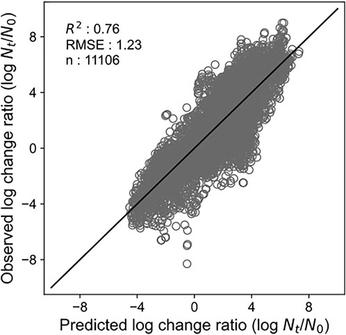
FIGURE 1. Comparison of the predicted and observed log change ratio for all the test data. The solid line represents residuals = 0.

FIGURE 2

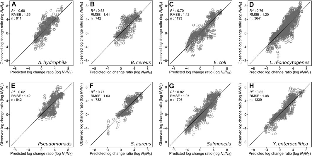
FIGURE 2. Comparison of the predicted and observed log change ratio for test data of Aeromonas hydrophila (A), Bacillus cereus (B), Escherichia coli (C), Listeria monocytogenes (D), Pseudomonads (E), Staphylococcus aureus (F), Salmonella (G), and Yersinia enterocolitica (H). The solid line represents residuals = 0.

FIGURE 3

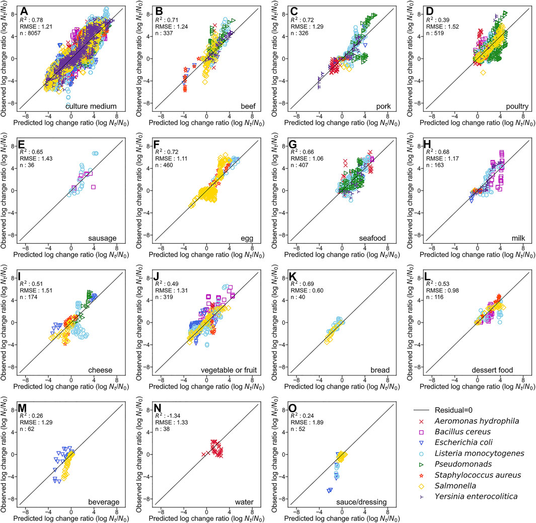
FIGURE 3. Comparison of the predicted and observed log change ratio for test data of culture medium (A), beef (B), pork (C), poultry (D), sausage (E), egg (F), seafood (G), milk (H), cheese (I), vegetable or fruit (J), bread (K), dessert food (L), beverage (M), water (N), and sauce/dressing (O). The solid line represents residuals = 0.

3.2 2D color plot visualization of bacterial behaviors

We introduced new 2D visualizations to illustrate the bacterial growth/survival ratio using combinations of temperature, pH, and a_w. Figure 4 shows a color map of eight bacterial behaviors in the broth after 10 days when the initial number was 4 log CFU/g. The limiting a_w value of growth for S. aureus was 0.90, whereas that for most microorganisms was an a_w value of 0.91 or above. The minimum pH value of B. cereus for growth was estimated to be 5.0, whereas that of many other organisms was 4.0–4.5. All eight bacteria grew when the pH was greater than 5.5. Some examples of 2D color maps, such as temperature–a_w and pH–temperature, can be found in the Supplementary Information. We compared the observed growth/no-growth experiment of L. monocytogenes in a culture medium at 25°C (Koutsoumanis et al., 2004) and our 2D map prediction. As shown in Figure 5, the validity of the 2D plots was visually confirmed.

FIGURE 4

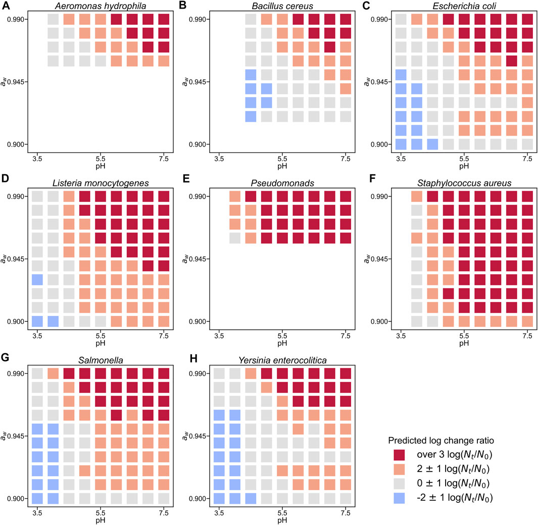
FIGURE 4. Change ratio from initial cell counts in broth at 20°C with an initial concentration of 4 log CFU/g after 10 days for Aeromonas hydrophila (A), Bacillus cereus (B), Escherichia coli (C), Listeria monocytogenes (D), Pseudomonads (E), Staphylococcus aureus (F), Salmonella (G), and Yersinia enterocolitica (H). Each square plot represents the value of the log change ratio ($\mathit{log}{N}_t/N_0$). Plot area by an organism is defined by the range of pH/a_w in the dataset. No-plots area represents outside of train and test data range.

FIGURE 5

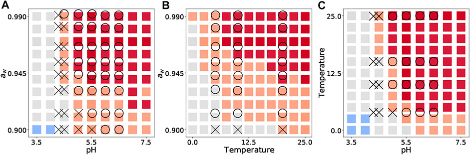
FIGURE 5. Comparison between observed growth ($○$) and no-growth (☓) and predicted change ratio from initial cell counts in a broth of Listeria monocytogenes after 30 days at 25°C (A), with pH 5.47–5.58 (B) with a_w of 0.965–0.967 (C). Experimental data were taken from Koutsoumanis et al. (2004). Each square plot represents the value of the log change ratio ($\mathit{log}{N}_t/N_0$); dark red is “strongly increased” (change > 3-log cycle), red is “increased” (change of 2 ± 1 log cycle), grey is “survival” (change of 0 ± 1 log cycle), and blue is “decreased” (change of −2 ± 1 log cycle).

3.3 Interpretation of the model

3.3.1 Feature importance

We calculated the feature importance to obtain the explanatory variable that was important in terms of contribution to the prediction performance in model development. Figure 6 shows the feature importance of the developed XGBoost model. The importance of each feature represents the ratio of the importance of each feature when the sum of all feature importance values is 1. “Initial cell number,” “Time,” and “a_w” contributed the most to model development and to almost the same extent. A categorical variable “Organism” representing the name of bacteria contributed to model development mostly to the same extent as the numerical variables “pH” and “Temperature.” Information regarding food, such as food category and name, also contributed to model development. All features contributed to the model development to some extent.

FIGURE 6

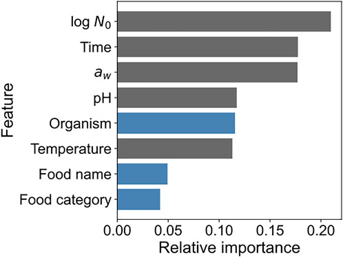
FIGURE 6. Feature importance of the developed XGBoost model. The x-axis indicates the relative importance, and the y-axis indicates the feature names. Blue and gray bars indicate categorical and numerical variables, respectively.

3.3.2 SHAP value

To see the model interpretability in a deeper perspective (i.e., the relationship between each environmental condition and the bacterial growth), we introduced the SHAP framework. The SHAP values for the three environmental features were calculated to determine the contribution of the environmental factors to bacterial growth. The SHAP value explains the contribution of each variable to the predicted $\mathit{log}{N}_t/N_0$ value of an instance. Positive and high SHAP values indicate that the feature value positively affected the predicted $\mathit{log}{N}_t/N_0$. Conversely, negative and low SHAP values imply that the feature value has a negative effect. The absolute SHAP value indicates the effect size of the environmental factors. Figure 7 shows the SHAP-dependence plots for a_w, pH, and temperature. The higher the a_w, the higher the SHAP value for a_w (Figure 7A). The SHAP value for temperature followed a similar relationship as that of a_w (Figure 7C). However, the SHAP value for pH was the highest when the pH value was approximately 7 (Figure 7B). According to the results of the SHAP dependency for each environmental factor, several trends in bacterial behavior could be suggested. When the value of a_w was greater than 0.95, the a_w positively affected bacterial growth. When the pH was approximately 7, it positively influenced bacterial growth. When the pH was less than 5.0, the low pH negatively influenced bacterial growth. When the temperature was 10–25°C, it positively influenced bacterial growth.

FIGURE 7

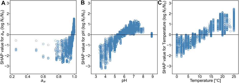
FIGURE 7. SHapley Additive eXplanations (SHAP) dependency plots for water activity (A), pH (B), and temperature (C).

4 Discussion

In the present study, we demonstrated the application of a data mining approach to predict bacterial population behavior using the ComBase database (Figures 1–3) and visualized these as 2D maps (Figure 4). Categorical data such as organism, food category, and food name also contributed to the construction of the model to some extent in the developed model (Figure 6). In addition, we demonstrated the environmental effects on the growth of the bacterial population (Figure 7). The data mining approach allowed us to model and reveal the multidimensional relationship between bacterial population behavior and the food environment. We showed that a data-driven approach to analyzing accumulated data could be useful for addressing food safety issues.

Although the dataset used in this study consisted of numerical and categorical variables, using a machine learning algorithm enabled us to predict bacterial population behavior using a single predictive model (Figure 1). Unlike numerical variables, categorical variables (e.g., food category, food name, and organism) must be replaced with numerical data, such as dummy variables for numerical operations (Palaniappan and Awang, 2008; Kim and Hong, 2017). Statistical modeling makes it difficult to consider categorical data when multiple conditions exist, such as food names and environmental conditions (Kim and Hong, 2017; Hiura et al., 2021). In contrast, the machine learning model enabled the description of the relationship between the food environment and bacteria, which is difficult for statistical models or human hand definition owing to the high dimensionality. Additionally, we succeeded in extending the model proposed by Hiura et al. (2021) to include eight bacterial species and 15 food categories.

We visualized the bacterial population behavior based on the idea of panoramic evaluation of the whole trend of the microbial response to various conditions. Our 2D map visualization showed a combination of factors that prevented bacterial growth (Figure 4). Compared to the literature data, our 2D color map can describe trends of population behavior of Listeria monocytogenes to the same extent (Figure 5), which supports the validity of our color map. Similar to our study, Ratkowsky & Ross (1995) proposed a growth/no-growth interface model. The growth/no growth interface models estimate the probability of bacterial growth and find combinations of factors preventing growth. The growth/no growth interface has been widely used in previous studies in predictive microbiology (Tienungoon et al., 2000; McKellar and Lu, 2001; Le Marc et al., 2005; Polese et al., 2011; Coroller et al., 2012; Kuroda et al., 2019). This approach was used to determine whether bacteria can grow easily under a wide range of experimental conditions. However, this interface cannot express the details of the bacterial population density. In the present study, we succeeded in evaluating not only whether there was growth or not, but also the change in bacterial population density (Figure 4). Our visualizing method helps us understand the bacterial concentration in various conditions at glance. Our visualization methods can be useful for developing processes that provide information for realistic estimations of food safety risks. Thus, our 2D map models are important for the dissemination of food safety regulations.

The SHAP value describes the contribution of each explanatory variable to each predicted $\mathit{log}{N}_t/N_0$. A positive SHAP value indicates bacterial growth. A negative SHAP value indicates a decrease in a bacterial population. We succeeded in mining information regarding the relationship between bacterial growth and environmental conditions from the dataset (Figure 7). These results mostly conform to the general opinion in food microbiology. For many food-spoilage and food-poisoning bacteria such as E. coli, Pseudomonas spp., and B. cereus, minimum a_w values for growth are approximately 0.95 (Jay et al., 2008a). The a_w value positively affected bacterial growth if it was greater than approximately 0.95. The optimal pH range for bacterial growth was approximately 7 (Figure 7A). Most food-spoilage and food-poisoning bacteria grow poorly as the pH decreases, especially below 3.5 (Adams and Nicolaides, 1997; Jay et al., 2008a). Similarly, the pH values could be used to predict bacterial population growth in the range of 6–7, whereas they worked negatively under pH 5 (Figure 7B). In addition, most foodborne microorganisms grow well at 20–45°C, and many bacterial species, except psychotropic bacteria or psychrophiles, cannot grow below 7°C (Jay et al., 2008a; Jay et al., 2008b). Similarly, temperature contributes to bacterial growth at more than approximately 10°C (Figure 7C). We showed a negative effect on bacterial growth by computing the SHAP value. The associations detected here replicate the well-known characteristics of bacterial growth in food microbiology, which supports the validity of our results and the possibility of utilizing data mining to extract bacterial population behavior.

Although our study uses data-driven methods to analyze the experimental data in the ComBase database with some advantages and expectations, it also has some limitations. Our model is not assumed to predict the ecology of microorganisms, because the ComBase database mainly focuses on bacterial growth and inactivation of only one type of bacterial species for each experiment for simplification. In the future, the competitive microbial condition would be analyzed with the dataset containing the ecology of microorganisms by data driven methods.

5 Conclusion

Data mining predicted the population behavior of eight foodborne pathogens and spoilage bacteria in the 15 food environments. In addition, growth inhibition owing to the food environment was quantitatively evaluated using data-driven methods. Our approach enabled us to extract useful information regarding food safety from a large amount of experimental data. The bacterial population behavior predicted by this procedure can provide guidelines for determining food processing and storage conditions. The main findings of this study support the data mining approach as valuable in the field of food microbiology.

Data availability statement

The original contributions presented in the study are included in the article/Supplementary Material, further inquiries can be directed to the corresponding author.

Author contributions

JH, JS, SN, SK, and KK conceptualized the study. JH, JS, SN, and KK designed the computation. JH and JS analyzed the data. JH wrote the python script and the first draft of the manuscript. All authors reviewed the manuscript.

Funding

This work was also supported by Kieikai Research Foundation and Tobe Maki scholarship Foundation (to KK), the Japan Science and Technology Agency Center of Innovation Program (grant number: JPMJCE1301), CREST (JPMJCR20H4), and JSPS KAKENHI (JP20H00425, JP21K19813) (to SN).

Conflict of interest

The authors declare that the research was conducted in the absence of any commercial or financial relationships that could be construed as a potential conflict of interest.

Publisher’s note

All claims expressed in this article are solely those of the authors and do not necessarily represent those of their affiliated organizations, or those of the publisher, the editors and the reviewers. Any product that may be evaluated in this article, or claim that may be made by its manufacturer, is not guaranteed or endorsed by the publisher.

Supplementary material

The Supplementary Material for this article can be found online at: https://www.frontiersin.org/articles/10.3389/frfst.2022.979028/full#supplementary-material

References

Adams, M. R., and Nicolaides, L. (1997). Review of the sensitivity of different foodborne pathogens to fermentation. Food control. 8 (5–6), 227–239. doi:10.1016/s0956-7135(97)00016-9

CrossRef Full Text | Google Scholar

Agius, R., Brieghel, C., Andersen, M. A., Pearson, A. T., Ledergerber, B., Cozzi-Lepri, A., et al. (2020). Machine learning can identify newly diagnosed patients with CLL at high risk of infection. Nat. Commun. 11 (1), 363–417. doi:10.1038/s41467-019-14225-8

PubMed Abstract | CrossRef Full Text | Google Scholar

Baranyi, J., Tamplin, M., and Ross, T. (2004). The ComBase initiative. Microbiol. Aust. 25 (3), 32. doi:10.1071/ma04332

CrossRef Full Text | Google Scholar

Bidlas, E., Du, T., and Lambert, R. J. W. (2008). An explanation for the effect of inoculum size on MIC and the growth/no growth interface. Int. J. Food Microbiol. 126 (1–2), 140–152. doi:10.1016/j.ijfoodmicro.2008.05.023

PubMed Abstract | CrossRef Full Text | Google Scholar

Chang, Y. C., Chang, K. H., and Wu, G. J. (2018). Application of eXtreme gradient boosting trees in the construction of credit risk assessment models for financial institutions. Appl. Soft Comput. 73, 914–920. doi:10.1016/j.asoc.2018.09.029

CrossRef Full Text | Google Scholar

Chen, T., and Guestrin, C. (2016). XGBoost: A scalable tree boosting system. Proceedings of the ACM SIGKDD International Conference on Knowledge Discovery and Data Mining. ACM, New York, NY, USA. 2016, 785–794. doi:10.1145/2939672.2939785

CrossRef Full Text | Google Scholar

Cios, K. J., and William Moore, G. (2002). Uniqueness of medical data mining. Artif. Intell. Med. 26 (1–2), 1–24. doi:10.1016/S0933-3657(02)00049-0

PubMed Abstract | CrossRef Full Text | Google Scholar

Coroller, L., Kan-King-Yu, D., Leguerinel, I., Mafart, P., and Membre, J. M. (2012). Modelling of growth, growth/no-growth interface and nonthermal inactivation areas of Listeria in foods. Int. J. Food Microbiol. 152 (3), 139–152. doi:10.1016/j.ijfoodmicro.2011.09.023

PubMed Abstract | CrossRef Full Text | Google Scholar

Cortez, P., Cerdeira, A., Almeida, F., Matos, T., and Reis, J. (2009). Modeling wine preferences by data mining from physicochemical properties. Decis. Support Syst. 47 (4), 547–553. doi:10.1016/j.dss.2009.05.016

CrossRef Full Text | Google Scholar

Delen, D., Walker, G., and Kadam, A. (2005). Predicting breast cancer survivability: A comparison of three data mining methods. Artif. Intell. Med. 34 (2), 113–127. doi:10.1016/j.artmed.2004.07.002

PubMed Abstract | CrossRef Full Text | Google Scholar

den Besten, H. M. W., and Zwietering, M. H. (2012). Meta-analysis for quantitative microbiological risk assessments and benchmarking data. Trends Food Sci. Technol., 34–39. doi:10.1016/j.tifs.2011.12.004

CrossRef Full Text | Google Scholar

Deringer, V. L., Bartok, A. P., Bernstein, N., Wilkins, D. M., Ceriotti, M., and Csanyi, G. (2021). Gaussian process regression for materials and molecules. Chem. Rev. 121, 10073–10141. doi:10.1021/acs.chemrev.1c00022

PubMed Abstract | CrossRef Full Text | Google Scholar

Doyle, M. P., Diez-Gonzalez, F., and Hill, C. (2019). Food microbiology: Fundamentals and frontiers. Food Microbiol. Fundam. Front. doi:10.1002/9781683670476

CrossRef Full Text | Google Scholar

Friedman, J. H. (2001). Greedy function approximation: A gradient boosting machine. Ann. Stat. 29 (5), 1189–1232. doi:10.1214/aos/1013203451

CrossRef Full Text | Google Scholar

Gould, G. W. (1996). Methods for preservation and extension of shelf life. Int. J. Food Microbiol. 33 (1), 51–64. doi:10.1016/0168-1605(96)01133-6

PubMed Abstract | CrossRef Full Text | Google Scholar

Gulyaeva, M., Huettmann, F., Shestopalov, A., Okamatsu, M., Matsuno, K., Chu, D. H., et al. (2020). Data mining and model-predicting a global disease reservoir for low-pathogenic Avian Influenza (A) in the wider Pacific rim using big data sets. Sci. Rep. 10 (1), 16817–16911. doi:10.1038/s41598-020-73664-2

PubMed Abstract | CrossRef Full Text | Google Scholar

Hand, D. J. (1998). Data mining: Statistics and more? Am. Stat. 52 (2), 112–118. doi:10.1080/00031305.1998.10480549

CrossRef Full Text | Google Scholar

Hiura, S., Koseki, S, and Koyama, K. (2021). Prediction of population behavior of Listeria monocytogenes in food using machine learning and a microbial growth and survival database. Sci. Rep. 11 (1), 10613. doi:10.1038/s41598-021-90164-z

PubMed Abstract | CrossRef Full Text | Google Scholar

Hochachka, W. M., Caruana, R., Fink, D., Munson, A., Riedewald, M., Sorokina, D., et al. (2007). Data-mining discovery of pattern and process in ecological systems. J. Wildl. Manage. 71 (7), 2427. doi:10.2193/2006-503

CrossRef Full Text | Google Scholar

Jagannath, A., and Tsuchido, T. (2003). ‘Predictive microbiology: A review’, biocontrol science. Japan: The Society for Antibacterial and Antifungal Agents, 1–7. doi:10.4265/bio.8.1

CrossRef Full Text | Google Scholar

Jay, J. M., Loessner, M. J., and Golden, D. A. (2008a). “Intrinsic and extrinsic parameters of foods that affect microbial growth,” in Modern food microbiology (Springer US), 39–59. doi:10.1007/0-387-23413-6_3

CrossRef Full Text | Google Scholar

Jay, J. M., Loessner, M. J., and Golden, D. A. (2008b). “Protection of foods with low-temperatures, and characteristics of psychrotrophic microorganisms,” in Modern food microbiology (Springer US), 395–413. doi:10.1007/0-387-23413-6_16

CrossRef Full Text | Google Scholar

Jiménez-Carvelo, A. M., et al. (2019). Alternative data mining/machine learning methods for the analytical evaluation of food quality and authenticity – a review. Food Res. Int. Elsevier Ltd, 25–39. doi:10.1016/j.foodres.2019.03.063

PubMed Abstract | CrossRef Full Text | Google Scholar

Kim, K., Hong, J. S, Yun, K. Y., Han, S. E., Kim, E. S., Kwon, B. S., et al. (2017). Laparoscopically assisted suprapubic surgery for adnexal tumors under epidural anesthesia. Minim. Invasive Ther. Allied Technol. 98, 39–43. doi:10.1080/13645706.2016.1223695

PubMed Abstract | CrossRef Full Text | Google Scholar

Koh, H. C., and Tan, G. (2005). Data mining applications in healthcare. J. Healthc. Inf. Manag. 19 (2), 64–72. doi:10.4314/ijonas.v5i1.49926

PubMed Abstract | CrossRef Full Text | Google Scholar

Koutsoumanis, K. P., Kendall, P. A., and Sofos, J. N. (2004). A comparative study on growth limits of Listeria monocytogenes as affected by temperature, pH and aw when grown in suspension or on a solid surface. Food Microbiol. 21 (4), 415–422. doi:10.1016/j.fm.2003.11.003

CrossRef Full Text | Google Scholar

Koutsoumanis, K. P., and Sofos, J. N. (2005). Effect of inoculum size on the combined temperature, pH and aw limits for growth of Listeria monocytogenes. Int. J. Food Microbiol. 104 (1), 83–91. doi:10.1016/j.ijfoodmicro.2005.01.010

PubMed Abstract | CrossRef Full Text | Google Scholar

Kuroda, S., Okuda, H., Ishida, W., and Koseki, S. (2019). Modeling growth limits of Bacillus spp. spores by using deep-learning algorithm. Food Microbiol. 78, 38–45. doi:10.1016/j.fm.2018.09.013

PubMed Abstract | CrossRef Full Text | Google Scholar

Le Marc, Y., Pin, C., and Baranyi, J. (2005). “Methods to determine the growth domain in a multidimensional environmental space,” in International journal of food microbiology (Elsevier), 3–12. doi:10.1016/j.ijfoodmicro.2004.10.003

PubMed Abstract | CrossRef Full Text | Google Scholar

Leistner, L. (2000). “Basic aspects of food preservation by hurdle technology,” in International journal of food microbiology (Elsevier), 181–186. doi:10.1016/S0168-1605(00)00161-6

PubMed Abstract | CrossRef Full Text | Google Scholar

Lundberg, S. M., Erion, G. G., and Lee, S.-I. (2018). Consistent individualized feature attribution for tree ensembles. Available at:https://arxiv.org/abs/1802.03888v3 (Accessed: January 21, 2022).

Google Scholar

Lundberg, S. M., and Lee, S. I. (2017). “A unified approach to interpreting model predictions,” in Advances in neural information processing systems, 4766–4775. Available at:https://github.com/slundberg/shap (Accessed: September 28, 2021).

Google Scholar

Mangalathu, S., Hwang, S. H., and Jeon, J. S. (2020). Failure mode and effects analysis of RC members based on machine-learning-based SHapley Additive exPlanations (SHAP) approach. Eng. Struct. 219, 110927. doi:10.1016/j.engstruct.2020.110927

CrossRef Full Text | Google Scholar

Mataragas, M., Rantsioua, K., Alessandria, V., and CocoLin, L. (2015). Estimating the non-thermal inactivation of Listeria monocytogenes in fermented sausages relative to temperature, pH and water activity. Meat Sci. 100, 171–178. doi:10.1016/j.meatsci.2014.10.016

PubMed Abstract | CrossRef Full Text | Google Scholar

McKellar, R. C., and Lu, X. (2001). A probability of growth model for Escherichia coli O157:H7 as a function of temperature, pH, acetic acid, and salt. J. Food Prot. 64 (12), 1922–1928. doi:10.4315/0362-028X-64.12.1922

PubMed Abstract | CrossRef Full Text | Google Scholar

McQuestin, O. J., Shadbolt, C. T., and Ross, T. (2009). Quantification of the relative effects of temperature, pH, and water activity on inactivation of Escherichia coli in fermented meat by meta-analysis. Appl. Environ. Microbiol. 75 (22), 6963–6972. doi:10.1128/AEM.00291-09

PubMed Abstract | CrossRef Full Text | Google Scholar

Mohanty, S. D., Lekan, D., McCoy, T. P., Jenkins, M., and Manda, P. (2022). Machine learning for predicting readmission risk among the frail: Explainable AI for healthcare. Patterns 3 (1), 100395. doi:10.1016/j.patter.2021.100395

PubMed Abstract | CrossRef Full Text | Google Scholar

Moncada-Torres, A., van Maaren, M. C., Hendriks, M. P., Siesling, S., and Geleijnse, G. (2021). Explainable machine learning can outperform Cox regression predictions and provide insights in breast cancer survival. Sci. Rep. 11 (1), 6968–7013. doi:10.1038/s41598-021-86327-7

PubMed Abstract | CrossRef Full Text | Google Scholar

Ndraha, N., Hsiao, H. I., Hsieh, Y. Z., and Pradhan, A. K. (2021). Predictive models for the effect of environmental factors on the abundance of Vibrio parahaemolyticus in oyster farms in Taiwan using extreme gradient boosting. Food control. 130, 108353. doi:10.1016/j.foodcont.2021.108353

CrossRef Full Text | Google Scholar

Nguyen, M., Long, S. W., McDermott, P. F., Olsen, R. J., Olson, R., Stevens, R. L., et al. (2019). Using machine learning to predict antimicrobial MICs and associated genomic features for nontyphoidal Salmonella. J. Clin. Microbiol. 57 (2), 012600–e1318. doi:10.1128/JCM.01260-18

PubMed Abstract | CrossRef Full Text | Google Scholar

Nychas, G.-J., Sims, E., Tsakanikas, P., and Mohareb, F. (2021). Data science in the food industry. Annu. Rev. Biomed. Data Sci. 4 (1), 341–367. doi:10.1146/annurev-biodatasci-020221-123602

PubMed Abstract | CrossRef Full Text | Google Scholar

Palaniappan, S., and Awang, R. (2008). Intelligent heart disease prediction system using data mining techniques. AICCSA 08 - 6th IEEE/ACS International Conference on Computer Systems and Applications. IEEE, Doha, Qatar 108–115. doi:10.1109/AICCSA.2008.449352431 March 2008 - 04 April 2008

CrossRef Full Text | Google Scholar

Polese, P., Del Torre, M., Spaziani, M., and Stecchini, M. L. (2011). A simplified approach for modelling the bacterial growth/no growth boundary. Food Microbiol. 28 (3), 384–391. doi:10.1016/j.fm.2010.09.011

PubMed Abstract | CrossRef Full Text | Google Scholar

Rodrigo, H., Beukes, E. W., Andersson, G., and Manchaiah, V. (2021). Exploratory data mining techniques (decision tree models) for examining the impact of internet-based cognitive behavioral therapy for tinnitus: Machine learning approach. J. Med. Internet Res. 23 (11), e28999. doi:10.2196/28999

PubMed Abstract | CrossRef Full Text | Google Scholar

Ross, S. R. P. J., Friedman, N. R., Dudley, K. L., Yoshimura, M., Yoshida, T., and Economo, E. P. (2018). Listening to ecosystems: Data-rich acoustic monitoring through landscape-scale sensor networks. Ecol. Res. 33 (1), 135–147. doi:10.1007/s11284-017-1509-5

CrossRef Full Text | Google Scholar

Ross, T., and McMeekin, T. A. (1994). Predictive microbiology. Int. J. Food Microbiol. 23 (3–4), 241–264. doi:10.1016/0168-1605(94)90155-4

PubMed Abstract | CrossRef Full Text | Google Scholar

Shehadeh, A., Alshboul, O., Al Mamlook, R. E., and Hamedat, O. (2021). Machine learning models for predicting the residual value of heavy construction equipment: An evaluation of modified decision tree, LightGBM, and XGBoost regression. Automation Constr. 129, 103827. doi:10.1016/j.autcon.2021.103827

CrossRef Full Text | Google Scholar

Skandamis, P. N., Stopforth, J. D., Kendall, P. A., Belk, K. E., Scanga, J. A., Smith, G. C., et al. (2007). Modeling the effect of inoculum size and acid adaptation on growth/no growth interface of Escherichia coli O157:H7. Int. J. Food Microbiol. 120 (3), 237–249. doi:10.1016/j.ijfoodmicro.2007.08.028

PubMed Abstract | CrossRef Full Text | Google Scholar

Tienungoon, S., Ratkowsky, D. A., McMeekin, T. A., and Ross, T. (2000). Growth limits of Listeria monocytogenes as a function of temperature, pH, NaCl, and lactic acid. Appl. Environ. Microbiol. 66 (11), 4979–4987. doi:10.1128/AEM.66.11.4979-4987.2000

PubMed Abstract | CrossRef Full Text | Google Scholar

Wang, L., Wang, X., Chen, A., Jin, X., and Che, H. (2020). Prediction of type 2 diabetes risk and its effect evaluation based on the xgboost model. Healthc. Switz. 8 (3), 247. doi:10.3390/healthcare8030247

PubMed Abstract | CrossRef Full Text | Google Scholar

Yang, S., and Liu, M. (2021). Mining meta-indicators of university ranking: A machine learning approach based on SHAP. Available at: https://arxiv.org/abs/2111.12526v1 (Accessed: January 7, 2022).

Google Scholar

Zoabi, Y., Kehat, O., Lahav, D., Weiss-Meilik, A., Adler, A., and Shomron, N. (2021). Predicting bloodstream infection outcome using machine learning. Sci. Rep. 11 (1), 20101–20111. doi:10.1038/s41598-021-99105-2

PubMed Abstract | CrossRef Full Text | Google Scholar