Flapping about: trends and drivers of Australian cownose ray (Rhinoptera neglecta) coastal sightings at their southernmost distribution range

1 Introduction

Understanding the distribution and habitat use patterns of elusive marine species is key to informing effective management and conservation strategies. This is especially true for elasmobranchs, which have conservative life histories and are facing unprecedented pressure from anthropogenic activities (1). The distribution, movement, and behavior of elasmobranchs are often complex and difficult to elucidate due to the myriad of potential biotic and abiotic drivers of habitat use (2, 3). Biotic influences encompass the need to forage and find suitable prey (4–6), predator avoidance (7), reproduction (8), and symbiotic relationships (9, 10). In addition, a range of abiotic factors can also influence the occurrence and behavior of elasmobranchs, including sea temperature (11, 12), tidal and lunar cycles (9, 13–15), salinity gradients (16, 17), rainfall (18, 19), barometric pressure (20, 21), and dissolved oxygen (22).

In coastal ecosystems, oceanographic processes, such as western boundary currents (e.g., the East Australian Current, EAC) regulate local abiotic factors, including sea temperature and current velocity, whilst also influencing nutrient enrichment via upwelling events (23, 24). Along Australia's east coast, these oceanographic processes are known to influence the distribution and movement of elasmobranchs (25–27). For example, manta rays (Mobular alfredi) exploit productive waters upwelled by a mesoscale eddy that forms as the EAC flows past the southern Great Barrier Reef (5, 9, 25). Considering the projected environmental impacts of climate change (28, 29), identifying the drivers of species' distributions is imperative for the development of management strategies to protect vulnerable populations or life stages (e.g., gravid females or juveniles) and evaluate how their distributions and behaviors may shift with changing oceans.

The Rhinopteridae (cownose rays), Aetobatidae (eagle rays), and Mobulidae (devil and manta rays) families of the order Myliobatiformes (Chondrichthyes: Batoidea) are often referred to as pelagic rays, as they typically occupy epipelagic waters (30, 31) and use coastal regions to forage (32) or for courtship and reproduction (33). Cownose and eagle rays are durophagous taxa and frequently aggregate in groups or “fevers” that can range from just a few individuals to thousands of rays (34, 35). For example the American cownose ray, Rhinoptera bonasus, has been observed in groups comprising several thousand individuals (36, 37). Whilst the function of these aggregations likely varies spatially and temporally for each species, the formation of groups inevitably influences the distribution and behavior of these rays. Therefore, understanding the function of aggregations and how they influence the distribution and movement of species may provide vital information on biological processes such as the location of mating, pupping, or foraging grounds, and intra-specific patterns of habitat use.

Due to the unpredictable and transient behavior of some durophagous pelagic rays, there are few opportunities for observations and field research. As a result, there is a limited understanding of the basic biology and ecology of many species, particularly relating to their habitat use and movement, impeding their management and conservation (38). Typically, the coastal occurrence of durophagous rays is seasonal, with observations occurring most often during warmer months (34, 39–41). However, the occurrence and movement of durophagous rays is complex and can vary between ocean basins and conspecifics (42–46). To date, there have been no large-scale studies focusing on durophagous pelagic rays for the south-western Pacific Ocean.

The Australian cownose ray (Rhinoptera neglecta) (47) is a pelagic ray that primarily occurs along the north and east coasts of Australia and in the Indo-Pacific region (30, 38). The species is currently classified as Data Deficient on the International Union for the Conservation of Nature's Red List of Threatened Species, with substantial knowledge gaps pertaining to its biology, life history, behavior, distribution, and habitat use (38). Recent stable isotope analyses revealed an overlapping isotopic niche with A. ocellatus, likely due to their co-occurrence along the east coast of Australia and similar foraging ecologies (48). Seasonal variations of R. neglecta occurrence along sections of Australia's east coast have previously been reported using fishery catch rate data (41, 49, 50) and a regionally limited study using drones (35). However, the species' relative abundance and drivers of occurrence have not been explored across larger latitudinal scales such as the east coast of Australia.

This study examined trends in the seasonality, spatio-temporal distribution, and relative abundance of R. neglecta observed along the coast of NSW during multi-year helicopter surveys operated via the state government. Using three generalized additive models, we assessed the drivers (temporal, spatial, oceanographic, meteorological, and tidal predictors) influencing (1) the presence-absence of R. neglecta along the coast of NSW, (2) the estimated group size of R. neglecta observed during offshore aerial surveys and (3) the estimated group size of R. neglecta observed during inshore aerial surveys.

2 Materials and methods

Observation data used in this study were obtained through marine wildlife monitoring helicopter surveys under the auspices of the NSW Department of Primary Industries (DPI) Shark Management Strategy to mitigate shark-human interactions (https://www.sharksmart.nsw.gov.au). All flights were covered by appropriate animal care and ethics through the NSW DPI Animal Care and Ethics Committee permit number 16/09.

2.1 Aerial surveys and R. neglecta sightings

From January 2017 through June 2019, sightings of R. neglecta were recorded by trained observers during 935 longshore helicopter surveys (Figure 1). Surveys were flown over seven regions along the NSW coastline (Figure 2) covering a total of approximately 980 km (~47%; Table 1). Each of the seven regions were flown by independent helicopters and crews who had received extensive marine wildlife identification training and were regularly accompanied by NSW DPI Fisheries staff with long-term aerial survey experience. Observers identified R. neglecta based on their golden colouration and unique body/head shape. Surveys were primarily done during NSW school holidays, which occur approximately every 10 weeks (Supplementary Table S1).

Figure 1

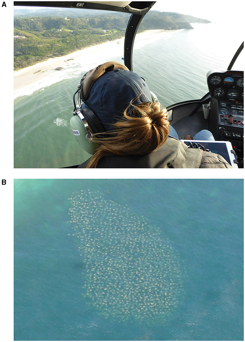
Figure 1. Images of (A) an observer using the purpose-built iPad application in a helicopter during a north-bound aerial survey, looking toward the coast and (B) a large group of Rhinoptera neglecta observed from a helicopter during an aerial survey.

Figure 2

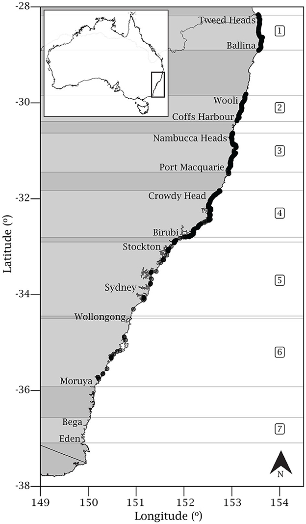
Figure 2. Map of the New South Wales coast highlighting the seven regions where helicopter survey flights were conducted from January 2017 through June 2019. Black dots represent sightings of Rhinoptera neglecta (n = 1324). Region 1 – Tweed Heads to Ballina; region 2 – Wooli to Coffs Harbor; region 3 – Nambucca Heads to Port Macquarie; region 4 – Crowdy Head to Birubi; region 5 – Stockton to south Wollongong; region 6 – south Wollongong to Moruya, and region 7 – Bega to Eden. See Table 1 for additional information for each region.

Table 1

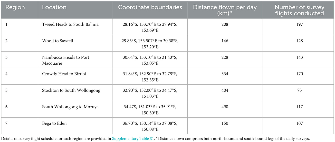
Table 1. Regions and distances surveyed along the New South Wales coastline where aerial surveys were conducted.

Survey flights were conducted once a day, starting at 07:30, and consisted of a north-bound and south-bound leg covering the same stretch of coastline. Flights began with the north-bound leg which was flown 500 m offshore to enable a search of the area immediately beyond the last line of waves (known as the “backline” by surfers). During the north-bound leg, observers looked toward the coast from the front left seat to reduce the effect of sun glare whilst ensuring the maximum 300 m strip width recommended by Robbins et al. (51). On completion of the north-bound leg, the helicopter landed to allow the crew to rest and refuel the helicopter, plus allow animal movement in and out of the transect strip width. After an hour, the south-bound leg, with a track line over the beach, was initiated with the observer facing seaward from the front left seat and searching inshore (or nearshore) within a 300 m strip width from the beach out to sea. Duration of flights were dependent on the stretch of coastline surveyed for each region, with the max flight time for a single north- or south-bound leg ranging from 50 min in smaller regions (e.g., regions 2 and 7) to 2.5 h in larger regions (e.g., regions 5 and 6; Table 1). Survey flights were weather dependent, and data were only collected when sea state was less than category 4 on the Beaufort scale to ensure wind-induced white caps were not a hindrance for observer identification of marine wildlife [see (52)].

Helicopters were flown at an average speed of 100 knots (185 km h⁻¹) and altitude of 500 feet (152 m). Observers used an iPad (Apple, United States, www.apple.com) and a purpose-made data collection application known as “SharkSmart PRO,” to record sightings of R. neglecta. Date, time of day, latitude, and longitude were autogenerated for each sighting and estimates of group size (as a numeric value) and notes of weather and environmental conditions were logged in real time for each sighting by the observer.

Sighting data were subject to quality control processes to remove entries with missing fields, seemingly incorrect location coordinates (e.g., where the reported sighting location fell over land), or cases of ambiguous estimates of group size (i.e., where no numeric value was supplied). In total of 1,324 sighting records were retained and compiled in a dataset, hereafter referred to as group size data, which included all sightings of R. neglecta from all survey regions, each with corresponding sighting data (date, time, latitude, and longitude), group size estimate, and whether the sighting occurred during the north- or south-bound leg. To assess trends in sightings and account for variations in the size of regions, the average number of sightings per kilometer flown were calculated for each region as well as for the offshore and inshore surveys of each region.

To analyse R. neglecta occurrence, a presence-absence dataset was compiled using the sighting records and a schedule of helicopter survey flights for each region. For each daily survey flight conducted in each region, a score of 1 or 0 was allocated depending on whether a sighting of R. neglecta had been recorded (1 indicated the presence of R. neglecta on said date in the region of interest and 0 represented the absence of R. neglecta). Where the species was present (at least one individual observed), the corresponding sighting data were retained. For consistency, in cases of multiple sightings per day for a single region, only the data of the earliest sighting of the day were used to extract environmental data. Since time and location were autogenerated by the “SharkSmart PRO” application for each sighting, absence records did not have a corresponding time or location. For all absence records, location was approximated as the median latitude for the corresponding region, with longitude occurring within 500 m of the coastline, as would be surveyed by the helicopter crews.

2.2 Predictors

A suite of predictor variables were sourced for each sighting record in the presence-absence and group size datasets to identify seasonal trends and potential drivers of R. neglecta occurrence and group size along the NSW coast. Since the location of absence records was the same latitude and longitude for each of the seven regions, only environmental predictors that did not rely on fine-scale location could be used with the presence-absence dataset. Time of day was not considered as a predictor because flights only occurred in the morning. As a result, seven and nine environmental predictors were sourced for the presence-absence and group size datasets, respectively (Table 2).

Table 2

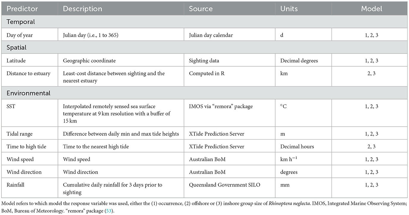
Table 2. Summary of predictors used in the generalized additive models with a brief description of each predictor, its data source, units, and which model the predictor was used in.

Day of year was derived from the Julian day calendar and has the capacity to infer monthly and austral seasonal trends, where summer is December to February, autumn is March to May, winter is June to August and spring is September to November.

Latitude has been correlated to occurrence and distribution patterns of numerous species, including sharks and rays with large spatial distributions (19, 54, 55). The NSW coast spans ~9^o of latitude in a temperate zone that is heavily influenced by local and mesoscale (i.e., the EAC and its eddy field) processes (56, 57). Therefore, it was presumed the ecology of R. neglecta may be influenced by latitude and any associated fine-scale environmental processes occurring within the ~2,100 km length of coastline.

Daily interpolated remotely sensed sea surface temperature (SST) at 9 km resolution, sourced from the Integrated Marine Observing System (www.imos.org.au), were extracted using the extractEnv() function of the “remora” package (53). The date and location of each sighting record within the presence-absence and group size datasets were used to extract the corresponding SST.

Tide data were collected for a representative station within each region (Supplementary Table S2) from the XTide Prediction Server (https://tides.mobilegeographics.com/). The maximum daily tidal range (difference between the maximum and minimum daily tide heights) was calculated for each sighting record, and the time to the nearest high tide was determined using the time of day for each sighting. Moon phase was also considered as a predictor, however, those data strongly correlated with the tidal range data and were subsequently excluded from the models.

Nutrient loading and estuarine output is suggested as a possible reason for variation in faunal assemblages off beaches in northern NSW (58). To assess whether this could be a factor influencing group size of R. neglecta, the shortest, least-cost distance to the nearest estuary (in both north and south directions) was computed in R (59) using the latitude and longitude of each sighting record and a high-resolution shapefile of NSW estuaries (60).

Rainfall was selected as a proxy for fluctuations in estuarine productivity and subsequent prey availability, under the presumption that higher rainfall would result in increased riverine output and nutrient loading within nearby estuaries, which may influence local sightings of R. neglecta. Along the east coast of Australia, rainfall influences the abundance and movement of other elasmobranchs (e.g., manta rays and bull sharks) up to eight days after a heavy rainfall event (5, 18, 19, 61). As such, the cumulative rainfall for the seven days prior to each sighting was extracted from the Queensland Government's SILO database daily rainfall product (62) in R. The date and location (with a 5 km buffer) for each sighting were used to extract the corresponding rainfall data.

Wind data were obtained from the Australian Bureau of Meteorology (BoM) using a representative weather station for each region (Supplementary Table S2). BoM's three-hour synoptic data provided wind speed and wind direction for the closest hour to each sighting record, except for region 3 and 4, where data were only available for 09:00. Wind direction was measured in degrees and indicated the direction from which the wind was blowing. Values of 0 and 360 degrees represent winds coming from the north (i.e., northerly winds or winds blowing southward).

2.3 Modeling approach

Generalized additive models (GAM) were used to assess the effect of predictors on the occurrence and group size of R. neglecta using the “mgcv” R package (63). Correlations between each of the environmental predictors for each of the datasets were assessed (Pearson correlation coefficient) and predictors were only retained if the correlation coefficient was ≤ 0.6 and if there were no strong non-linear correlations visible in raw scatterplots to ensure predictors were not highly correlated with each other.

2.3.1 Model 1: occurrence of R. neglecta along the NSW coast

Model 1 used the observed presence or absence of R. neglecta along the NSW coast for each survey day as the response variable, with a log transformed offset of distance flown per day (Table 1), a logit link function and binomial error structure. The resulting occurrence model had the following structure:

$\begin{array}{l}g(E(Y))=\beta 0+f1(x1)+f2(x2)+\dots +fi(xi)\end{array}$

Where g represents a link function, β0 is the intercept and f i(xi) is a smoothing function for each variable with either the default thin plate regression spline or a cyclic cubic regression spline, depending on the nature of the data. See below for rationale on spline choice.

2.3.2 Model 2 and 3: offshore and inshore drivers of R. neglecta group size

Due to differences in the track line of north- (500 m offshore) and south-bound (along the water/beach interface) legs and a statistically significant difference in group size estimates between legs [GLMM with observation level random effect (64): estimate = 0.20, standard error = 0.08, Z = 2.36, P = 0.018; DHARMa nonparametric dispersion value = 0.87, P = 0.688; “DHARMa” package (65); Figure 3], these data were analyzed as two separate models. The north-bound data were used in model 2 (herein referred to as the offshore model) whilst the south-bound data were used in model 3 (herein referred to as the inshore model). These models used the estimated group size for each R. neglecta sighting as the response variable, with a log transformed offset of region length (i.e., the distance flown per survey leg; Table 1), a negative binomial error structure (to account for overdispersion) and log link function. These models were generalized additive mixed models (GAMM) and included two random effects. The first was called “observer group” to account for potential observer bias in estimating group size, but this also incorporated some regional effects since each region had its own crew of observers. The second was “survey” to account for non-independence of sightings that were recorded during the same aerial survey flight (i.e., on the same day and in the same region).

Figure 3

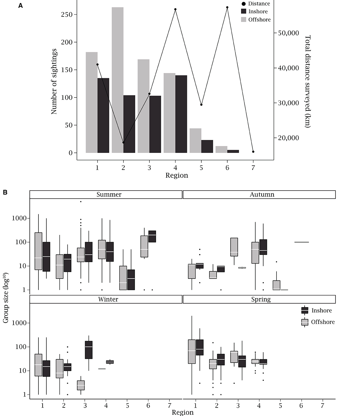
Figure 3. (A) The total number of Rhinoptera neglecta sightings (n = 1324) with total distance flown (each north- and south-bound survey legs combined) throughout the study period for each region and (B) group sizes (on a log¹⁰ transformed y-axis) estimated by observers per region and season, pooled across all years. Black boxes represent groups observed inshore (during south-bound legs of survey flights) and gray boxes indicate groups observed offshore (during north-bound legs). Box plots depict the median (white line), inter-quartile range (25th and 75th percentile as bottom and top of box, respectively), 95% confidence intervals (vertical whiskers), and outliers (points).

The offshore and inshore group size models had the following structure:

$\begin{array}{l}g(E(Y))=\beta 0+ai+f1(x1)+f2(x2)+\dots +fi(xi)\end{array}$

Where g represents a link function, β0 is the intercept, αi represents random effects (i.e., observer group and survey) and f i(xi) is a smoothing function for each variable (either the default thin plate regression spline or a cyclic cubic regression spline).

To build each model, initially a null model and single-variable models for each predictor (Table 2) were constructed. Based on the single-variable models, predictors that were significant (P = < 0.05) were compared to the null model using Akaike Information Criterion (AIC) scores. The predictor with the lowest AIC score was incorporated into the model (Supplementary Table S3) and a Pearson correlation test was used to assess the predictor's relationship with all remaining predictors (accepted level of correlation: correlation coefficient ≤ 0.6). This was repeated for all predictors until the AIC scores of remaining predictors were higher than the preceding model, at which point all predictors yet to be added to the final model were excluded to achieve parsimony. Latitude and day of year were incorporated into the models as an interaction with a full tensor product spline because differing environmental conditions are expected between latitudinal bands and seasons. Cyclic predictors such as day of year, wind direction, and time to high tide had cyclic splines applied in all models. Knots for all predictors were originally set to 5 to avoid overfitting and were adjusted where necessary to optimize fitting (Supplementary Table S3). To calculate the individual contribution of predictors in the final model, the deviance explained of the model without the predictor was deducted from the deviance explained of the full model whilst maintaining the smoothing parameter of the predictor of interest.

3 Results

3.1 Survey effort

A total of 935 helicopter survey flights, each with a north- and south-bound leg, were conducted across the seven coastal regions of NSW from January 2017 through June 2019. The number of survey flights varied between regions and seasons (Figure 4). Region 1 had the highest total number of flights (197) whilst region 5 had the fewest (66). Flights were most frequent during summer and autumn because the high volume of beachgoers during these seasons prompts more consistent flight schedules (Supplementary Table S1). During summer, the number of flights was highest in regions 7 and 6; however, no flights were conducted in these regions during winter and spring or in region 5 during winter.

Figure 4

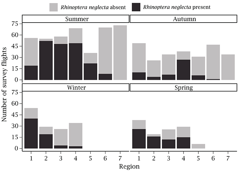
Figure 4. Number of survey flights (n = 935) conducted in each region per season, pooled across all years. Black bars indicate flights where Rhinoptera neglecta were present along the coast of New South Wales and gray bars represent flights where Rhinoptera neglecta were not observed.

3.2 Presence of R. neglecta along the NSW coast

Rhinoptera neglecta were present along the NSW coastline during 41.39% of the total survey flights conducted across the seven regions (R. neglecta were present on 387 days). Most of the sightings occurred in the northern half of NSW, in region 1, 4, and 2 (95, 94, and 90 occurrences, respectively). However, regions 2 and 4 had the highest percentage of sightings per flights conducted (70.31 and 55.29% of each respective region's flights). R. neglecta were present during only 12.46% of the flights conducted in regions 5, 6, and 7 combined. No R. neglecta occurred in region 7 even though 107 survey flights were conducted.

There were clear seasonal patterns in the species' presence along the NSW coast (Figure 4). During summer, R. neglecta were observed most often in regions 2, 3, and 4 (48 to 51 sightings each). The same regions also had the highest percentage of sightings per flights conducted during summer (region 2 = 94.44%, region 3 = 82.76%, and region 4 = 71.01%), whilst region 1 and 6 had the lowest percentage of sightings per flights conducted (33.93% of 56 flights and 11.43% of 70 flights, respectively). During winter, the presence of R. neglecta was highest in region 1 (74.07% of 54 flights) and decreased as the regions progressed southward (Figure 4).

3.3 Drivers of R. neglecta presence along the NSW coast

The final iteration of the occurrence GAM retained the interaction between day of year and latitude, wind direction, rainfall, SST, tidal range, and wind speed (Figures 5A–F) and explained 44.20% of the deviance in the presence-absence of R. neglecta along the coast of NSW. The interaction between day of year and latitude contributed the majority of the deviance explained (38.21%; Figure 5A), followed by wind direction (9.03%; Figure 5B) and rainfall (1.78%; Figure 5C), although only the latitude and day of year interaction, and rainfall were significant. All other predictors contributed < 1% each (Figures 5D–F; Supplementary Table S4). The model indicated that R. neglecta were more likely to be present in the northern regions of NSW during warmer months (i.e., summer and spring), with very few occurrences in the three southern regions throughout the year (Figure 5A). The model also suggested the likelihood of the species being present decreased with increasing rain in the seven days prior to the aerial survey (Figure 5C) and increased with winds coming from the northwest (270–360/0 degrees; Figure 5B).

Figure 5

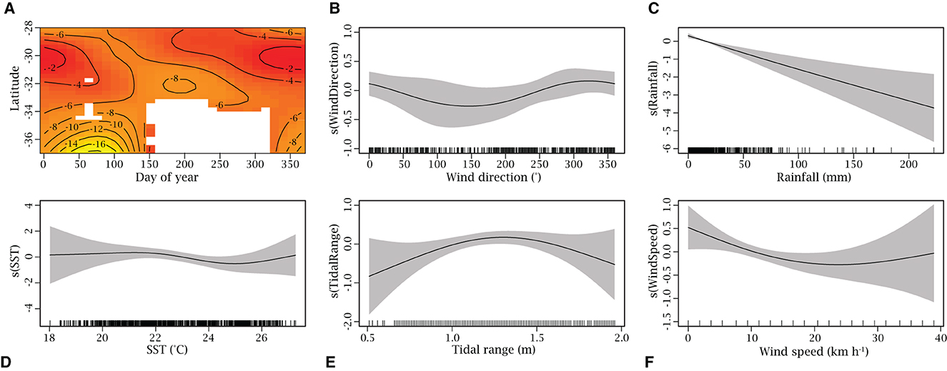
Figure 5. Generalized additive model assessing the drivers of Rhinoptera neglecta occurrence (presence/absence) along the New South Wales coast (n = 387). Predictor variables are (A) interaction of latitude and day of year, (B) wind direction (°), (C) rainfall (mm), (D) sea surface temperature (SST) (°C), (E) tidal range (m), and (F) wind speed (km h⁻¹) and are presented in order of their contribution to the model's deviance explained. The scale of the y-axis varies between each plot and indicates the relative effect of that predictor on the presence-absence of R. neglecta. Dashes on x-axis shows the distribution of data and gray shaded areas represent the 95% confidence interval. In (A) the latitude and day of year interaction plot, red indicates higher values and yellow indicates lower values. White space in the latitude and day of year interaction plot indicates no interpolation was performed due to a lack of data with this combination of variables.

3.4 Sightings and group size of R. neglecta

During the survey flights that R. neglecta were present, the species was recorded 1,324 times, with an estimated total of 92,597 R. neglecta individuals recorded. This value is likely an overestimate since some groups and individuals may have been double counted between survey legs. Overall, region 2 had the highest average number of sightings per kilometer (0.23), with other regions ranging 0–0.17 sightings per kilometer. When categorized by season, there was a clear latitudinal trend in average sightings per kilometer for summer, winter and spring, where sightings were most frequent in northern regions and then decreased with the southward progression of regions (Figure 6). Region 2 had the highest average sightings per kilometer during summer, with more sightings during the offshore survey leg. However, during autumn, winter and spring, average sightings per kilometer were more similar between regions 1 and 2 (Figure 6).

Figure 6

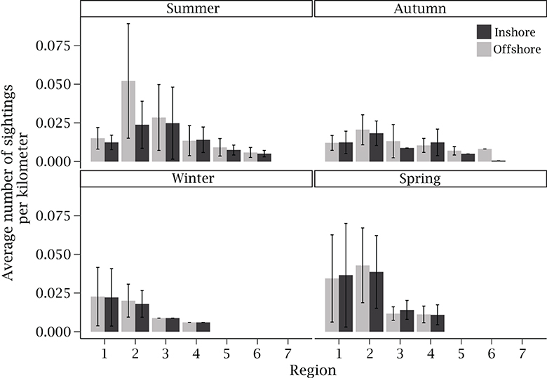
Figure 6. Average (± standard deviation) number of Rhinoptera neglecta sightings per kilometer flown during offshore (gray) and inshore (black) aerial surveys along the coast of New South Wales. Sightings are categorized by region and season and pooled across all years (n = 1,324).

In every region, there were flights during which R. neglecta were sighted multiple times. This occurred most often in regions 2 and 3, where multiple sightings occurred during 74.44 and 73.24% of the flights where R. neglecta were present. The most sightings in a single flight occurred in region 1, where 22 sightings (10 offshore and 12 inshore) yielded a total estimate of 2,989 individual rays (1,306 offshore and 1,683 inshore). The greatest number of sightings in a single day across all regions was 28 (offshore only) and included at least one sighting from regions 1–6. The maximum number of R. neglecta observed on a single day across all regions was 6,791 individuals (5,101 offshore and 1,690 inshore) observed in regions 2–5. The majority of these rays were a single group estimated to consist of 5,000 individuals observed in region 3.

Across all regions, the average (± standard deviation) estimated group size was 70 ± 194 rays. The southernmost region where R. neglecta were observed (region 6) had the highest average group size of 131 ± 119 rays (from 17 sightings) and was higher than northern regions which had the highest frequency of sightings and/or sightings per kilometer (region 1 average group size of 317 sightings = 108 ± 215 rays; region 2 average group size of 367 sightings = 23 ± 28 rays).

Sightings mostly consisted of groups comprising 11–99 rays (51.81%), followed by groups with < 10 rays (29.23%), and schools up to 500 individuals (16.69%; Figure 7). Groups that consisted of 1000 and >1000 individuals made up 1.59% and 0.68% of sightings, respectively. Groups of all sizes were observed in regions 1, 3, and 4 (Figure 7). Sightings in region 2, which had the highest number of sightings per kilometer almost entirely (97.28%) comprised groups of < 100 individuals and there were no groups over 500 individuals.

Figure 7

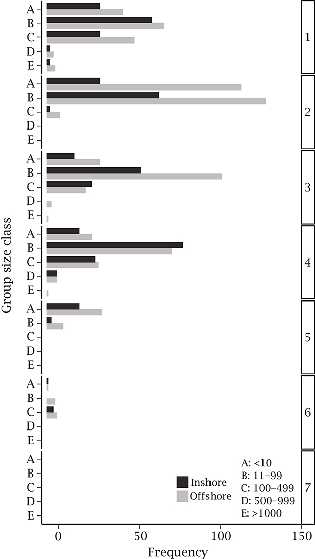
Figure 7. Frequency of Rhinoptera neglecta group size classes observed during aerial survey flights along the coast of New South Wales, categorized by region and pooled across all years. Black bars indicate groups observed inshore, during the south-bound leg of survey flights (n = 510). Gray bars indicate groups observed offshore, during the north-bound leg of survey flights (n = 814).

There were distinct differences in sightings and group size estimates between the inshore and offshore survey legs. Across all regions, the majority of sightings occurred offshore (814 sightings; 61.48%; Figure 3A), which also had the higher average estimated group size (73 ± 229 rays) between the two survey legs (inshore: 510 sightings; average group size of 65 ± 115 rays). There were also some seasonal trends in these sightings, where offshore group size estimates were higher than those observed inshore for all seasons except autumn. When considering region, region 6 had the fewest sightings of R. neglecta (17 sightings) but 58.82% of those sightings were groups comprising 100–499 individuals. This resulted in region 6 having the highest median group size estimate during summer and autumn (Figure 3B). Typically, median group size estimates between inshore and offshore survey legs were comparable, however, in some regions during specific seasons there were substantial differences in group sizes (Figure 3B). The most notable differences in group sizes between the inshore and offshore survey legs were region 3 during winter and region 6 during summer, where group size estimates were higher during inshore surveys (region 3–101 and 3.5; region 6–200 and 50).

3.5 Drivers of R. neglecta group size along the NSW coast

3.5.1 Offshore model

The GAMM assessing the drivers of R. neglecta group size offshore (model 2) retained six predictors (the interaction of day of year and latitude, SST, time to high tide, rainfall, tidal range, and wind speed) in its final iteration (Figure 8A). The model explained 42.58% of the deviance in group size estimates of R. neglecta observed during the offshore leg of aerial surveys along the coast of NSW and all predictors were significant (Supplementary Table S4). The day of year and latitude interaction, SST, and observer group contributed the most deviance explained (28.76, 17.79, and 4.29%, respectively; Supplementary Table S4). The remaining predictors and random effect contributed < 2% each. To achieve parsimony, wind direction was not included in the final model since the AIC value of the model with wind direction was < 2 points lower than full model and the predictor was non-significant. The model indicated clear latitudinal and temporal patterns in R. neglecta group sizes during offshore surveys. Larger groups of R. neglecta were more likely to occur in southern regions during warmer months and when water temperatures were cooler (Figure 8A).

Figure 8

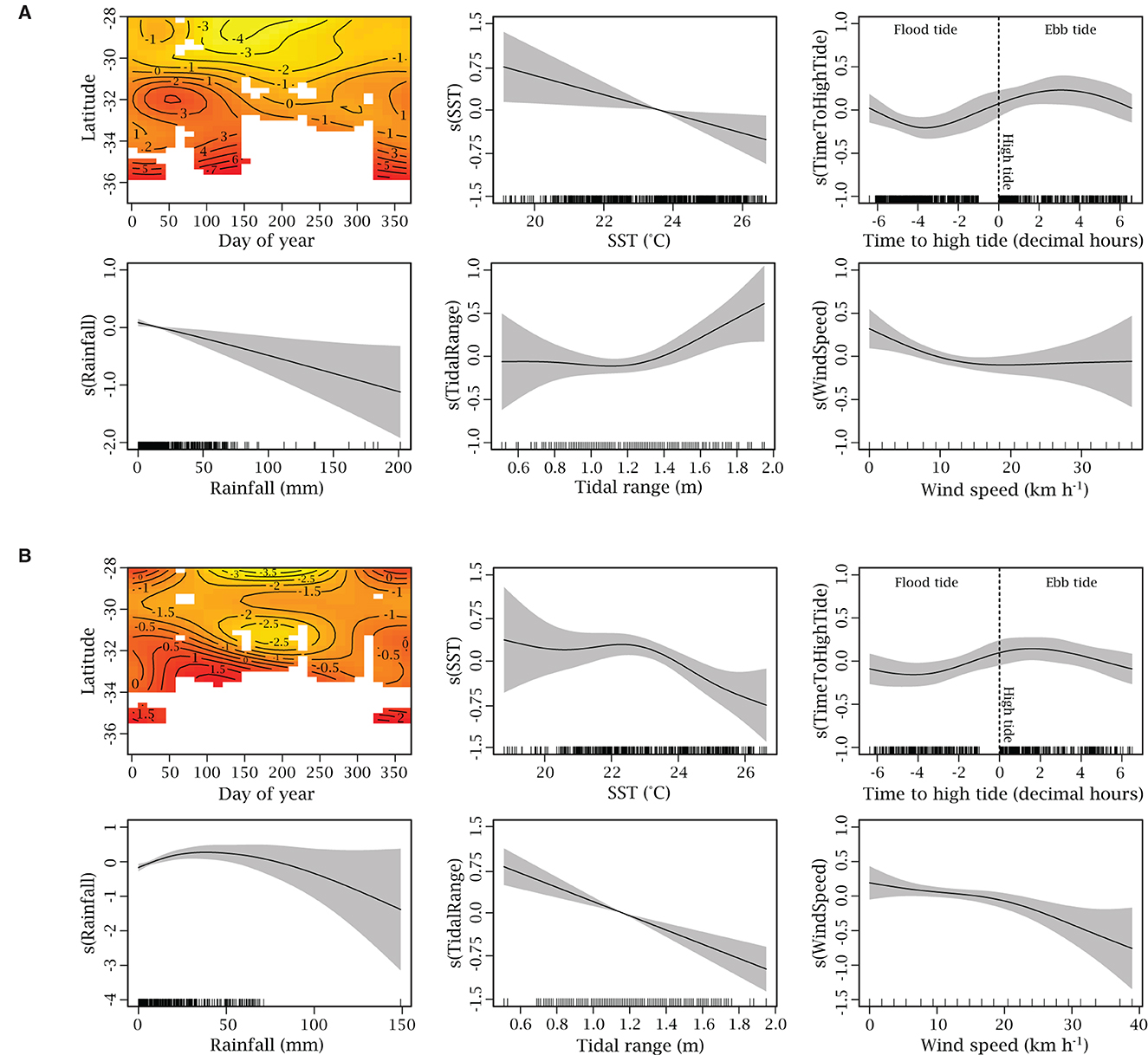
Figure 8. Generalized additive mixed models assessing the drivers of Rhinoptera neglecta estimated group size during (A) offshore and (B) inshore aerial surveys. Predictors are presented in the same order for easy comparison of the models. The scale of the y-axis varies for each plot and represents the relative effect of that predictor on the group size of R. neglecta. Dashes on x-axis shows the distribution of data and gray shaded areas represent the 95% confidence interval. Red shading in the latitude and day of year interaction plots indicates higher values and yellow shading indicates lower values. White space in the latitude and day of year interaction plot indicates no interpolation was performed due to a lack of data with this combination of variables.

3.5.2 Inshore model

The final iteration of the inshore group size model (model 3) was similar to the offshore model and retained the same six predictors which were the interaction between day of year and latitude, SST, time to high tide, rainfall, tidal range, and wind speed (Figure 8B). The inshore model indicated similar latitudinal and temporal trends in group sizes as the offshore model, such that larger groups were more likely to occur in southern regions during warmer months. The model also suggested larger groups of R. neglecta were likely to occur inshore when wind speeds were lower (< 10 km h⁻¹), during periods when tidal range was low (0.6–0.8 m) and in cooler waters, with group sizes reducing above 23^oC. The model explained 41.94% of the deviance in inshore group size estimates of R. neglecta along the coast of NSW, with the day of year and latitude interaction contributing the most (18.62%), followed by wind speed (3.89%), tidal range (2.45%), and SST (2.18%). All remaining predictors, including the observer group and survey random effects, contributed < 2% and were all significant, except for survey.

4 Discussion

This study represents the largest effort to date examining the occurrence patterns of R. neglecta at the southernmost extent of their known distribution. Using a multi-year aerial survey dataset of R. neglecta sightings along the NSW coastline and a generalized additive modeling framework, we analyzed the seasonal trends and drivers of the species' occurrence and group size to expand on current knowledge of their ecology in this region. Our results indicate that the presence of R. neglecta along the coast of NSW is primarily dependent on latitude and occurs on a seasonal basis. Similarly, the group size of R. neglecta also varied latitudinally, whereby on average groups are larger in southern regions. However, there can be a high abundance of rays in northern regions with groups that can contain several thousand individuals. Whilst the presence-absence and group size of R. neglecta are largely driven by latitude and seasonality, other environmental variables may influence occurrence patterns at finer scales (e.g., SST, rainfall, wind speed, and tidal flows).

To date, the reported distribution of R. neglecta extends from the tropical Indo-Pacific, along eastern Australia to Newcastle in central NSW [32.930°S; (30, 38)]. Additional anecdotal sightings of the species have been reported by members of the public via the Atlas of Living Australia (66) as far south as Sussex Inlet (35.150°S). The present study expands the known southern range of this poorly documented species by over 70 km (straight line distance), with sightings of R. neglecta as far south as 35.763°S (Wimbie Beach, Batemans Bay). Furthermore, this study supplies a baseline for the relative abundance of the species throughout the NSW region and reports at least 5,101 individual R. neglecta observed in a single day across all regions, during offshore surveys.

Tagliafico et al. (35) observed R. neglecta over a two-year period along a ~100 km of coastline in northern NSW (four of the five monitored beaches lie within region 1 of the present study) and recorded a total 5,979 R. neglecta. The largest observed group contained 412 individuals and occurred near a river mouth (35). The current study expands on the limited research regarding the species' relative abundance in northern NSW, reporting a total of 4,000 rays observed in region 1 on a single day (from offshore surveys only) which included a group estimated to consist of 2,000 individuals. Tagliafico et al. (35) found wind speed had a significant negative effect on the abundance of R. neglecta in groups. Wind speed was retained in all three of the models in the present study and broadly, our results align with those of Tagliafico et al. (35). We suggest that high wind speeds may decrease observer visibility and observability of rays due to surface disturbance and increased turbidity and/or the movement of R. neglecta offshore into deeper water when the surf zone may be more turbulent. Such weather conditions have been noted as issues in remotely measuring movement and behaviors of other rays (67) and sharks (68) along the east Australian coast.

The north-to-south nature of the NSW coastline allowed for an examination of latitudinal effects on sightings of R. neglecta. Results of the GAMM analyses highlighted day of year and latitude as strong influences on both coastal sightings of R. neglecta and group size, suggesting that sightings of the species were more likely to occur at northern latitudes, but groups were more likely to be larger at southern latitudes. R. neglecta were reliably and relatively evenly observed across surveys conducted in the northern regions of the NSW coast (i.e., regions 1 to 4). South of 32.5°S, R. neglecta were observed much less frequently, with a gradual decrease in the detection of the species and no sightings recorded in region 7. These results suggest that R. neglecta primarily occupy tropical and sub-tropical waters, with the ability to move to more temperate latitudes when sea temperatures allow. The southernmost region where the species was observed (i.e., region 6) consistently hosted large groups comprising between 50 and 500 rays. Together, these latitudinal patterns may indicate a mass migration phenomenon whereby individual rays gather up in larger schools as they travel south. The rays may also only visit the more southern sites as large groups, potentially due to the energetic benefits of traveling in schools (69). Rhinoptera spp. undertake seasonal, mass, coastal migrations, with sea temperatures being the presumed trigger for migratory behaviors (37, 70, 71). However, the thermal thresholds that trigger the egress behavior of Rhinoptera bonasus, range from 16^oC in the Atlantic Ocean (42) to 20^oC in the Gulf of Mexico (16). Here, all three models suggested that R. neglecta were more likely to be present and in larger groups when SSTs are cooler, around 21–23°C, which may indicate a similar thermal trigger for these events in NSW. A similar temperature threshold also applies to other Myliobatiform rays, such as spotted eagle rays in the Gulf of Mexico that occur when water temperature ranges 23–31^oC (34). In their respective studies, Blaylock (37) and Schwartz (70) hypothesized that such large, migrating aggregations of cownose rays were unlikely to be feeding related and may be aimed at maximizing mate encounter success and reproduction. Future research efforts in NSW are required to elucidate R. neglecta behavior and foraging ecology at the southern swathes of their distribution to better understand latitudinal influences.

Rhinoptera neglecta sightings occurred throughout the year in coastal waters of NSW, albeit more frequently and in higher abundances during the warmer months (i.e., austral summer and spring). These results support the concept that R. neglecta may be seasonally migrating to the NSW coast and aggregating en masse during the warmer months. There is also evidence to suggest seasonal migrations to the southern range of the NSW coast could facilitate parturition, mating and courtship as multiple gravid females have been captured in nets during summer in region 5 (Chan, unpublished data). Further investigations into the timing and behaviors of individuals in large aggregations in each survey region will help shed more light onto potential motivations underpinning this phenomenon.

Rhinoptera neglecta are reported as highly abundant further to the north along the Queensland and northern NSW coasts (35, 58). This study corroborates these observations. Whilst the majority of groups observed here were relatively small (< 100 rays) with occasional groups of up to 500 rays, larger aggregations, estimated to comprise up to ~5,000 individuals, were also reported in several of the surveyed regions. Unfortunately, the sparse and sporadic nature of these observations prevented detailed investigations into these “super fevers.” It is worth noting that the irregular effort associated with these aerial surveys (i.e., mainly conducted during school holidays and with different flight schedules between regions) prevented a robust examination of seasonal dynamics of R. neglecta occurrence in coastal waters of NSW and may have biased some of the seasonal trends observed. It is also important to note that the group size estimates reported here are likely conservative as Rhinoptera spp. are known to stack, with a single group comprising several layers of rays (35, 70), which aerial observers may be unable to quantify from above.

Whilst it was expected that larger groups of R. neglecta would be observed during the offshore survey legs due to the bathymetry (i.e., deeper waters would be more conducive to larger groups), there were regions where inshore median group size estimates were higher than offshore during every season. It is plausible that some of these groups are utilizing the surf zone for foraging. However, on 10 occasions (in regions 1 and 4), groups estimated to contain > 500 individuals were observed inshore, and it thus seems unlikely that there would be ample prey to support a group this size if the function is purely foraging. Although, in the Gulf of Mexico, increases in R. bonasus abundance can coincide with spikes in benthic prey densities (72).

It is hypothesized that groups of R. neglecta may also be aggregating in shallower waters for courtship/mating, parasite removal and/or protection from predators. There is evidence of courtship and mating behaviors of pelagic myliobatiform rays (R. bonasus and A. narinari) in shallow coastal waters (33); however, these typically only include a few individuals. Although R. neglecta could be partaking in a different form of parasite removal, such as rubbing against the substrate to dislodge external parasites, a behavior which has been observed in A. ocellatus (73), their regular occurrence in shallow sandy nearshore waters implies this is unlikely to be a primary driver for their use of this habitat. Inhabiting inshore shallow waters and aggregating in large groups may also provide some refuge to the smaller bodied R. neglecta from predators that prey on the species, such as great hammerhead sharks Sphyrna mokarran (74) or white sharks Carcharodon carcharias (75), as is the case for many small or juvenile fish species (49). Future research should investigate the behavior of individuals or groups closer to the shore to elucidate the function of inshore aggregations.

Based on the affinity of other cownose ray species to estuaries and river mouths (32, 76, 77), it was expected that sightings of R. neglecta in NSW would also be associated with these features as they typically provide safe refugia and abundant benthic prey (72, 78, 79). Surprisingly, the distance to estuary predictor did not make it into any of the models. It is important to note that estuary mouths typically have higher turbidity, especially after rainfall events, which may affect the ability of observers to sight the target species. Furthermore, boat traffic within estuaries may influence the diving behavior of these rays, causing them to dive deeper whilst transiting these areas. Acoustic or satellite tagging using pressure sensors may provide insights into the vertical movement of these rays within estuaries, along coastlines and in offshore habitats [e.g., (80, 81)]. In addition, it is worth noting that the GPS coordinates for each sighting were recorded by the “SharkSmart PRO” application via the cellular network whilst the helicopter flew at 185 km h⁻¹, which could have compromised the accuracy of some of these locations and therefore some of the fine-scale spatial patterns observed.

Considering the deviance explained for all three models was 41–44%, there are additional influences on the occurrences and group sizes of R. neglecta along the NSW coast that are yet to be identified. Several other environmental predictors were considered as part of this study, including chlorophyll-a concentration as a proxy for oceanic productivity (9, 82), salinity (22, 32), wave height (83), and habitat type (2, 11, 84). However, data for these predictors were not accessible in the present study due to a lack of coverage across temporal and spatial ranges or contamination of satellite derived data that could not be resolved to adequately reduce the number of gaps in the data. Current velocity and direction are of particular interest since current speeds can be used by marine organisms to reduce the cost of transport or to maximize opportunities to forage on diffuse prey (6, 69, 85, 86). It is possible that R. neglecta utilize ocean currents to save energy and travel efficiently during their regional migrations using the increased summer flow of the EAC (87, 88). Manta rays are known to maximize opportunities to forage on zooplankton when tidal currents and nutrient loads act to concentrate prey items (5, 6, 9). The diet of R. bonasus is diverse and encompasses crustaceans such as amphipods when available in sufficient quantities (72). Another Rhinoptera sp. was observed swimming amidst an aggregation of whale sharks actively feeding on zooplankton off Baja California Sur, Mexico (89). It is, therefore, possible that regional to fine-scale current dynamics along the NSW coastline, and the known upwelling events in this region (23, 90), may have influenced coastal prey availability and ultimately aggregations of R. neglecta. The aforementioned predictors should be explored in the future to refine findings from this study.

Despite considerable numbers of R. neglecta routinely caught in various fisheries and in bather protection programs off eastern Australia (91), there has been very little scientific interest in this species, which has resulted in important knowledge gaps regarding its basic biology and ecology. This study presents the largest aerial survey dataset of R. neglecta sightings off the NSW coast. Our results reveal new southernmost records for the species, extending its known distribution by 70 km to 35.763°S. We also report group sizes that are larger than those previously recorded for the species. Identifying patterns of distribution, abundance, and key environmental influences is crucial to improve management of the species and its habitat, particularly under the threats of continued fishing and climate change. Here we show that coastal occurrences and group sizes of R. neglecta off NSW are related to a set of key spatial, temporal, and environmental factors that operate over various scales with changes occurring with latitude and the distance of individuals to shore. This study provides a baseline for future research of R. neglecta that is urgently required to understand the ecological role of the species, to develop effective management strategies, and to assess potential implications associated with ongoing perturbations.

Data availability statement

The raw data supporting the conclusions of this article will be made available by the authors, without undue reservation.

Ethics statement

The animal study was approved by the NSW DPI Animal Care and Ethics Committee. The study was conducted in accordance with the local legislation and institutional requirements.

Author contributions

AC: Writing – original draft, Writing – review & editing, Formal analysis, Methodology. FJ: Conceptualization, Formal analysis, Supervision, Writing – review & editing. FM: Formal analysis, Methodology, Writing – review & editing. JW: Conceptualization, Funding acquisition, Supervision, Writing – review & editing. HS: Formal analysis, Writing – review & editing. AS: Data curation, Writing – review & editing. VP: Conceptualization, Data curation, Supervision, Writing – review & editing.

Funding

The author(s) declare financial support was received for the research, authorship, and/or publication of this article. This project was funded in part by the School of Natural Sciences, Macquarie University and the New South Wales Department of Primary Industries Fisheries Scientific Committee. AC was supported by the Macquarie University Research Training Program Scholarship.

Acknowledgments

We thank the observers and crews of the companies contracted to fly helicopter surveys on behalf of the NSW DPI Shark Management Strategy. We also thank A/Prof. Peter Petocz from the Department of Statistics, Macquarie University, for providing valuable advice on our data and modeling methodology and Dr. Amandine Schaeffer from the University of New South Wales for supplying the BoM wind data used in the analyses. SST data were sourced from Australia's Integrated Marine Observing System (IMOS) – IMOS is enabled by the National Collaborative Research Infrastructure Strategy (NCRIS). We thank the School of Natural Sciences at Macquarie University for partly funding this research and the Marine Ecology Group at Macquarie University for their support during this project.

Conflict of interest

The authors declare that the research was conducted in the absence of any commercial or financial relationships that could be construed as a potential conflict of interest.

The authors JW and FJ declared that they were an editorial board member of Frontiers, at the time of submission. This had no impact on the peer review process and the final decision.

Publisher's note

All claims expressed in this article are solely those of the authors and do not necessarily represent those of their affiliated organizations, or those of the publisher, the editors and the reviewers. Any product that may be evaluated in this article, or claim that may be made by its manufacturer, is not guaranteed or endorsed by the publisher.

Supplementary material

The Supplementary Material for this article can be found online at: https://www.frontiersin.org/articles/10.3389/frish.2023.1323633/full#supplementary-material

References

1. Dulvy N, Pacoureau N, Rigby CL, Pollom RA, Jabado RW, Ebert DA, et al. Overfishing drives over one-third of all sharks and rays toward a global extinction crisis. Curr Biol. (2021) 31:4773–87. doi: 10.1016/j.cub.2021.08.062

Crossref Full Text | Google Scholar

2. Speed CW, Field IC, Meekan MG, Bradshaw CJA. Complexities of coastal shark movements and their implications for management. Mar Ecol Prog Ser. (2010) 408:275–93. doi: 10.3354/meps08581

Crossref Full Text | Google Scholar

3. Schlaff AM, Heupel MR, Simpfendorfer CA. Influence of environmental factors on shark and ray movement, behaviour and habitat use: a review. Rev Fish Biol Fish. (2014) 24:1089–103. doi: 10.1007/s11160-014-9364-8

Crossref Full Text | Google Scholar

4. Heupel MR, Hueter RE. Importance of prey density in relation to the movement patterns of juvenile blacktip sharks (Carcharhinus limbatus) within a coastal nursery area. Mar Freshw Res. (2002) 53:543–50. doi: 10.1071/MF01132

Crossref Full Text | Google Scholar

5. Weeks SJ, Magno-Canto MM, Jaine FRA, Brodie J, Richardson AJ. Unique sequence of events triggers manta ray feeding frenzy in the southern Great Barrier Reef, Australia. Remote Sens. (2015) 7:3138–52. doi: 10.3390/rs70303138

Crossref Full Text | Google Scholar

6. Armstrong AO, Armstrong AJ, Jaine FRA, Couturier LIE, Fiora K, Uribe-Palomino J, et al. Prey density threshold and tidal influence on reef manta ray foraging at an aggregation site on the Great Barrier Reef. PLoS ONE. (2016) 11:e0153393. doi: 10.1371/journal.pone.0153393

PubMed Abstract | Crossref Full Text | Google Scholar

7. Vaudo JJ, Heithaus MR. Microhabitat selection by marine mesoconsumers in a thermally heterogeneous habitat: behavioral thermoregulation or avoiding predation risk? PLoS ONE. (2013) 8:e61907. doi: 10.1371/journal.pone.0061907

PubMed Abstract | Crossref Full Text | Google Scholar

8. Mourier J, Planes S. Direct genetic evidence for reproductive philopatry and associated fine-scale migrations in female blacktip reef sharks (Carcharhinus melanopterus) in French Polynesia. Mol Ecol. (2013) 22:201–14. doi: 10.1111/mec.12103

PubMed Abstract | Crossref Full Text | Google Scholar

9. Jaine FRA, Couturier LIE, Weeks SJ, Townsend KA, Bennett MB, Fiora K, et al. When giants turn up: sighting trends, environmental influences and habitat use of the manta ray Manta alfredi at a coral reef. PLoS ONE. (2012) 7:e46170. doi: 10.1371/journal.pone.0046170

PubMed Abstract | Crossref Full Text | Google Scholar

10. Armstrong AO, Armstrong AJ, Bennett MB, Richardson AJ, Townsend KA, Everett JD, et al. Mutualism promotes site selection in a large marine planktivore. Ecol E11. (2021) 5606–23. doi: 10.1002/ece3.7464

PubMed Abstract | Crossref Full Text | Google Scholar

11. Lee K, Smoothey AF, Harcourt RG, Roughan M, Butcher PA, Peddemors VM, et al. Environmental drivers of abundance and residency of a large migratory shark, Carcharhinus leucas, inshore of a dynamic western boundary current. Mar Ecol Prog Ser. (2019) 622:121–37. doi: 10.3354/meps13052

Crossref Full Text | Google Scholar

12. Smoothey AF, Gray CA, Kennelly SJ, Masens OJ, Peddemors VM, Robinson WA, et al. Patterns of occurrence of sharks in Sydney Harbour, a large urbanised estuary. PLoS ONE. (2016) 11:e0146911. doi: 10.1371/journal.pone.0146911

PubMed Abstract | Crossref Full Text | Google Scholar

13. O'Shea OR, Kingsford MJ, Seymour J. Tide-related periodicity of manta rays and sharks to cleaning stations on a coral reef. Mar Freshw Res. (2010) 61:65–73. doi: 10.1071/MF08301

Crossref Full Text | Google Scholar

14. Martins APB, Heupel MR, Bierwagen SL, Chin A, Simpfendorfer C. Diurnal activity patterns and habitat use of juvenile Pastinachus ater in a coral reef flat environment. PLoS ONE. (2020) 15:e0228280. doi: 10.1371/journal.pone.0228280

PubMed Abstract | Crossref Full Text | Google Scholar

15. Niella Y, Wiefels A, Almeida U, Jaquemet S, Lagabrielle E, Harcourt R, et al. Dynamics of marine predators off an oceanic island and implications for management of a preventative shark fishing program. Mar Biol. (2021) 168:42. doi: 10.1007/s00227-021-03852-9

Crossref Full Text | Google Scholar

16. Ajemian MJ, Powers SP. Seasonality and ontogenetic habitat partitioning of cownose rays in the northern Gulf of Mexico. Estuar Coasts. (2016) 39:1234–48. doi: 10.1007/s12237-015-0052-2

Crossref Full Text | Google Scholar

17. Schlaff AM, Heupel MR, Udyawer V, Simpfendorfer CA. Biological and environmental effects on activity space of a common reef shark on an inshore reef. Mar Ecol Prog Ser. (2017) 571:169–81. doi: 10.3354/meps12107

Crossref Full Text | Google Scholar

18. Niella Y, Smoothey AF, Taylor MD, Peddemors VM, Harcourt R. Environmental drivers of fine-scale predator and prey spatial dynamics in Sydney Harbour, Australia, and adjacent coastal waters. Estuar Coasts. (2022) 45:1465–79. doi: 10.1007/s12237-021-01020-2

Crossref Full Text | Google Scholar

19. Smoothey AF, Niella Y, Brand C, Peddemors VM, Butcher PA. Bull shark (Carcharhinus leucas) occurrence along beaches of south-eastern Australia: understanding where, when and why. Biol. (2023) 12:1189. doi: 10.3390/biology12091189

PubMed Abstract | Crossref Full Text | Google Scholar

20. Heupel MR, Simpfendorfer CA, Hueter RE. Running before the storm: blacktip sharks respond to falling barometric pressure associated with Tropical Storm Gabrielle. J Fish Biol. (2003) 63:1357–63. doi: 10.1046/j.1095-8649.2003.00250.x

Crossref Full Text | Google Scholar

21. Udyawer V, Chin A, Knip DM, Simpfendorfer CA, Heupel MR. Variable response of coastal sharks to severe tropical storms: environmental cues and changes in space use. Mar Ecol Prog Ser. (2013) 480:171–83. doi: 10.3354/meps10244

Crossref Full Text | Google Scholar

22. Craig JK, Gillikin PC, Magelnicki MA, May LN. Habitat use of cownose rays (Rhinoptera bonasus) in a highly productive, hypoxic continental shelf ecosystem. Fish Oceanogr. (2010) 19:301–17. doi: 10.1111/j.1365-2419.2010.00545.x

Crossref Full Text | Google Scholar

23. Roughan M, Middleton JH. A comparison of observed upwelling mechanisms off the east coast of Australia. Cont Shelf Res. (2002) 22:2551–72. doi: 10.1016/S0278-4343(02)00101-2

Crossref Full Text | Google Scholar

24. Armbrecht LH, Roughan M, Rossi V, Schaeffer A, Davies PL, Waite AM, et al. Phytoplankton composition under contrasting oceanographic conditions: upwelling and downwelling (Eastern Australia). Cont Shelf Res. (2014) 75:54–67. doi: 10.1016/j.csr.2013.11.024

Crossref Full Text | Google Scholar

25. Jaine FRA, Rohner CA, Weeks SJ, Couturier LIE, Bennett MB, Townsend KA, et al. Movements and habitat use of reef manta rays off eastern Australia: offshore excursions, deep diving and eddy affinity revealed by satellite telemetry. Mar Ecol Prog Ser. (2014) 510:73–86. doi: 10.3354/meps10910

Crossref Full Text | Google Scholar

26. Smoothey AF, Lee KA, Peddemors VM. Long-term patterns of abundance, residency and movements of bull sharks (Carcharhinus leucas) in Sydney Harbour, Australia. Sci Rep. (2019) 9:18864. doi: 10.1038/s41598-019-54365-x

PubMed Abstract | Crossref Full Text | Google Scholar

27. Niella Y, Smoothey AF, Peddemors V, Harcourt R. Predicting changes in distribution of a large coastal shark in the face of the strengthening East Australian Current. Mar Ecol Prog Ser. (2020) 642:163–77. doi: 10.3354/meps13322

Crossref Full Text | Google Scholar

28. Harley CDG, Hughes AR, Hultgren KM, Miner BG, Sorte CJB, Thornber CS, et al. The impacts of climate change in coastal marine systems. Ecol Lett. (2006) 9:228–41. doi: 10.1111/j.1461-0248.2005.00871.x

PubMed Abstract | Crossref Full Text | Google Scholar

29. Chin A, Kyne PM, Walker TI, McAuley RB. An integrated risk assessment for climate change: analysing the vulnerability of sharks and rays on Australia's Great Barrier Reef. Glob Change Biol. (2010) 16:1936–53. doi: 10.1111/j.1365-2486.2009.02128.x

Crossref Full Text | Google Scholar

30. Last PR, Stevens JD. Sharks and rays of Australia. Melbourne: CSIRO Publishing (1994).

Google Scholar

31. Aschliman NC. Interrelationships of the durophagous stingrays (Batoidea: Myliobatidae). Environ Biol Fishes. (2014) 97:967–79. doi: 10.1007/s10641-014-0261-8

Crossref Full Text | Google Scholar

32. Collins AB, Heupel MR, Simpfendorfer CA. Spatial distribution and long-term movement patterns of cownose rays Rhinoptera bonasus within an estuarine river. Estuar Coasts. (2008) 31:1174–83. doi: 10.1007/s12237-008-9100-5

Crossref Full Text | Google Scholar

33. McCallister M, Mandelman J, Bonfil R, Danylchuk A, Sales M, Ajemian M, et al. First observation of mating behavior in three species of pelagic myliobatiform rays in the wild. Environ Biol Fishes. (2020) 103:163–73. doi: 10.1007/s10641-019-00943-x

Crossref Full Text | Google Scholar

34. Bassos-Hull K, Wilkinson KA, Hull PT, Dougherty DA, Omori KL, Ailloud LE, et al. Life history and seasonal occurrence of the spotted eagle ray, Aetobatus narinari, in the eastern Gulf of Mexico. Environ Biol Fishes. (2014) 97:1039–56. doi: 10.1007/s10641-014-0294-z

Crossref Full Text | Google Scholar

35. Tagliafico A, Butcher PA, Colefax AP, Clark GF, Kelaher BP. Variation in cownose ray Rhinoptera neglecta abundance and group size on the central east coast of Australia. J Fish Biol. (2019) 96:427–33. doi: 10.1111/jfb.14219

PubMed Abstract | Crossref Full Text | Google Scholar

36. Clark E. Massive aggregations of large rays and sharks in and near Sarasota, Florida. Zoologica. (1963) 48:61–4. doi: 10.5962/p.203310

Crossref Full Text | Google Scholar

37. Blaylock R. A. (1989). A massive school of cownose rays, Rhinoptera bonasus (Rhinopteridae), in lower Chesapeake Bay, Virginia. Copeia: 744–748 doi: 10.2307/1445506

Crossref Full Text | Google Scholar

38. Jacobsen IP, Stevens J. Rhinoptera Neglecta. The IUCN Red List of Threatened Species. (2015) Available online at: https://www.iucnredlist.org/species/161530/68642171 (accessed April 4, 2023).

Google Scholar

39. Yamaguchi A, Kawahara I, Ito S. Occurrence, growth and food of longheaded eagle ray, Aetobatus flagellum, in Ariake Sound, Kyushu, Japan. Environ Biol Fishes. (2005) 74:229–38. doi: 10.1007/s10641-005-0217-0

Crossref Full Text | Google Scholar

40. Schluessel V, Bennett MB, Collin SP. Diet and reproduction in the white-spotted eagle ray Aetobatus narinari from Queensland, Australia and the Penghu Islands, Taiwan. Mar Freshw Res. (2010) 61:1278–89. doi: 10.1071/MF09261

Crossref Full Text | Google Scholar

41. Taylor S, Sumpton W, Ham T. Fine-scale spatial and seasonal partitioning among large sharks and other elasmobranchs in south-eastern Queensland, Australia. Mar Freshw Res. (2011) 62:638–47. doi: 10.1071/MF10154

Crossref Full Text | Google Scholar

42. Smith JW, Merriner JV. Age and growth, movements and distribution of the cownose ray, Rhinoptera bonasus, in Chesapeake Bay. Estuaries. (1987) 10:153–64. doi: 10.2307/1352180

Crossref Full Text | Google Scholar

43. Rogers C, Roden C, Lohoefener R, Mullin K, Hoggard W. Behavior, distribution, and relative abundance of cownose ray schools Rhinoptera bonasus in the northern Gulf of Mexico. Northeast Gulf Sci. (1990) 11:69–76. doi: 10.18785/negs.1101.08

Crossref Full Text | Google Scholar

44. Omori KL, Fisher RA. Summer and fall movement of cownose ray, Rhinoptera bonasus, along the east coast of United States observed with pop-up satellite tags. Environ Biol Fishes. (2017) 100:1435–49. doi: 10.1007/s10641-017-0654-6

Crossref Full Text | Google Scholar

45. Ogburn MB, Bangley CW, Aguilar R, Fisher RA, Curran MC, Webb SF, et al. Migratory connectivity and philopatry of cownose rays Rhinoptera bonasus along the Atlantic coast, USA. Mar Ecol Prog Ser. (2018) 602:197–211. doi: 10.3354/meps12686

Crossref Full Text | Google Scholar

46. DeGroot BC, Bassos-Hull K, Wilkinson KA, Lowerre-Barbieri S, Poulakis GR, Ajemian MJ, et al. Variable migration patterns of whitespotted eagle rays Aetobatus narinari along Florida's coastlines. Mar Biol 168. (2021) 18. doi: 10.1007/s00227-021-03821-2

Crossref Full Text | Google Scholar

47. Ogilby JD. On some Queensland fishes. Mem Queensl Mus. (1912) 1:26–65.

Google Scholar

48. Chan AJ, Raoult V, Jaine FRA, Peddemors VM, Broadhurst MK, Williamson JE, et al. Trophic niche of Australian cownose rays (Rhinoptera neglecta) and whitespotted eagle rays (Aetobatus ocellatus) along the east coast of Australia. J Fish Biol. (2022) 100:970–8. doi: 10.1111/jfb.15028

PubMed Abstract | Crossref Full Text | Google Scholar

49. Tobin AJ, Mapleston A, Harry AV, Espinoza M. Big fish in shallow water; use of an intertidal surf-zone habitat by large-bodied teleosts and elasmobranchs in tropical northern Australia. Environ Biol Fishes. (2014) 97:821–38. doi: 10.1007/s10641-013-0182-y

Crossref Full Text | Google Scholar

50. Broadhurst MK, Cullis BR. Mitigating the discard mortality of non-target, threatened elasmobranchs in bather-protection gillnets. Fish Res. (2020) 222:105435. doi: 10.1016/j.fishres.2019.105435

Crossref Full Text | Google Scholar

51. Robbins WD, Peddemors VM, Kennelly SJ, Ives MC. Experimental evaluation of shark detection rates by aerial observers. PLoS ONE. (2014) 9:e83456. doi: 10.1371/journal.pone.0083456

PubMed Abstract | Crossref Full Text | Google Scholar

52. Barham EG, Sweeney JC, Leatherwood S, Beggs RK, Barham CL. Aerial census of the bottlenose dolphin, Tursiops truncatus, in a region of the Texas coast. Fisheries Bulletin. (1980) 77:585–95.

Google Scholar

53. Jaine FRA, Jonsen I, Udyawer V, Dwyer R, Scales K, Maron F, et al. Remora: Rapid Extractions of Marine Observations for Roving Animals. Version 0, 7.1. (2021) Available online at: https://imos-animaltracking.github.io/remora/ (accessed October 30, 2022).

Google Scholar

54. Vianna GMS, Vooren CM. Distribution and abundance of the lesser electric ray Narcine brasiliensis (Olfers, 1831) (Elasmobranchii: Narcinidae) in southern Brazil in relation to environmental factors. Braz J Oceanogr. (2009) 57:105–12. doi: 10.1590/S1679-87592009000200003

Crossref Full Text | Google Scholar

55. Braccini M, Aires-da-Silva A, Taylor I. Incorporating movement in the modelling of shark and ray population dynamics: approaches and management implications. Rev Fish Biol Fish. (2016) 26:13–24. doi: 10.1007/s11160-015-9406-x

Crossref Full Text | Google Scholar

56. Schaeffer A, Roughan M, Jones EM, White D. Physical and biogeochemical spatial scales of variability in the East Australian Current separation from shelf glider measurements. Biogeosciences. (2016) 13:1967–75. doi: 10.5194/bg-13-1967-2016

Crossref Full Text | Google Scholar

57. Lee KA, Roughan M, Malcolm HA, Otway NM. Assessing the use of area- and time-averaging based on known de-correlation scales to provide satellite derived sea surface temperatures in coastal areas. Front Mar Sci. (2018) 5:261. doi: 10.3389/fmars.2018.00261

Crossref Full Text | Google Scholar

58. Kelaher BP, Colefax AP, Tagliafico A, Bishop MJ, Giles A, Butcher PA, et al. Assessing variation in assemblages of large marine fauna off ocean beaches using drones. Mar Freshw Res. (2020) 71:68–77. doi: 10.1071/MF18375

Crossref Full Text | Google Scholar

59. R Core Team. R: a language and environment for statistical computing. Vienna: R Foundation for Statistical Computing, Version 4, 2.1 (2023).

Google Scholar

60. Geoscience Australia. Geodata Coast 100 K. (2004) Available online at: https://data.gov.au/dataset/geodata-coast-100k-2004 (accessed August 9, 2022).

Google Scholar

61. Werry JM, Sumpton W, Otway NM, Lee SY, Haig JA, Mayer DG, et al. Rainfall and sea surface temperature: key drivers for occurrence of bull shark, Carcharhinus leucas, in beach areas. Global Ecol Conserv. (2018) 15:e00430. doi: 10.1016/j.gecco.2018.e00430

Crossref Full Text | Google Scholar

62. Jeffrey SJ, Carter JO, Moodie KB, Beswick AR. Using spatial interpolation to construct a comprehensive archive of Australian climate data. Environ Model Softw. (2001) 16:309–30. doi: 10.1016/S1364-8152(01)00008-1

Crossref Full Text | Google Scholar

63. Wood SN. Generalized Additive Models: An Introduction with R, 2nd Edn. Boca Raton, FL: Chapman and Hall/CRC Press.

Google Scholar

64. Harrison XA. Using observation-level random effects to model overdispersion in count data in ecology and evolution. PeerJ. (2014) 2:e616. doi: 10.7717/peerj.616

PubMed Abstract | Crossref Full Text | Google Scholar

65. Hartig F. DHARMa: Residual Diagnostics for Hierarchical (Multi-Level/Mixed) Regression Models. Version 0.4.6 (2022). Available online at: https://cran.r-project.org/web/packages/DHARMa/vignettes/DHARMa.html (accessed January 20, 2023).

Google Scholar

66. Atlas of Living Australia. Rhinoptera neglecta Species Page. (2023) Available online at: https://bie.ala.org.au/species/https://biodiversity.org.au/afd/taxa/5255f2b9-ab8e-4586-8283-27cfacef0d4e (accessed August 20, 2023).

Google Scholar

67. Oleksyn S, Tosetto L, Raoult V, Joyce KE, Williamson JE. Going batty: the challenges and opportunities of using drones to monitor the behaviour and habitat use of rays. Drones. (2021) 5:12. doi: 10.3390/drones5010012

Crossref Full Text | Google Scholar

68. Butcher PA, Colefax AP, Gorkin RAIII, Kajiura SM, López NA, Mourier J, et al. The drone revolution of shark science: a review. Drones. (2021) 5:8. doi: 10.3390/drones5010008

Crossref Full Text | Google Scholar

69. Fish FE. Energetics of swimming and flying in formation. Comments Theor Biol. (1999) 5:283–304.

Google Scholar

70. Schwartz FJ. Mass migratory congregations and movements of several species of cownose rays, genus Rhinoptera: a world-wide review. J Elisha Mitchell Sci Soc. (1990) 106:10–3.

Google Scholar

71. Bangley CW, Edwards ML, Mueller C, Fisher RA, Aguilar R, Heggie K, et al. Environmental associations of cownose ray (Rhinoptera bonasus) seasonal presence along the US Atlantic coast. Ecosphere. (2021) 12:e03743. doi: 10.1002/ecs2.3743

Crossref Full Text | Google Scholar

72. Ajemian MJ, Powers SP. Habitat-specific feeding by cownose rays (Rhinoptera bonasus) of the northern Gulf of Mexico. Environ Biol Fishes. (2012) 95:79–97. doi: 10.1007/s10641-011-9858-3

Crossref Full Text | Google Scholar

73. Berthe C, Lecchini D, Mourier J. Chafing behaviour on a patch of sandy bottom by ocellated eagle ray (Aetobatus ocellatus). Mar Biodiv. (2017) 47:379–80. doi: 10.1007/s12526-016-0463-8

Crossref Full Text | Google Scholar

74. Raoult V, Broadhurst MK, Peddemors VM, Williamson JE, Gaston TF. Resource use of great hammerhead sharks (Sphyrna mokarran) off eastern Australia. J Fish Biol. (2019) 95:1430–40. doi: 10.1111/jfb.14160

PubMed Abstract | Crossref Full Text | Google Scholar

75. Grainger R, Peddemors VM, Raubenheimer D, Machovsky-Capuska GE. Diet composition and nutritional niche breadth variability in juvenile white sharks (Carcharodon carcharias). Front Mar Sci. (2020) 7:422. doi: 10.3389/fmars.2020.00422

Crossref Full Text | Google Scholar

76. Blaylock RA. Distribution and abundance of the cownose ray, Rhinoptera bonasus, in Lower Chesapeake Bay. Estuaries. (1993) 16:255–63. doi: 10.2307/1352498

Crossref Full Text | Google Scholar

77. Collins AB, Heupel MR, Motta PJ. Residence and movement patterns of cownose rays Rhinoptera bonasus within a south-west Florida estuary. J Fish Biol. (2007) 71:1159–78. doi: 10.1111/j.1095-8649.2007.01590.x

Crossref Full Text | Google Scholar

78. Myers RA, Baum JK, Shepherd TD, Powers SP, Peterson CH. Cascading effects of the loss of apex predatory sharks from a coastal ocean. Science. (2007) 315:1846–50. doi: 10.1126/science.1138657

PubMed Abstract | Crossref Full Text | Google Scholar

79. Glaspie CN, Seitz RD. Role of habitat and predators in maintaining functional diversity of estuarine bivalves. Mar Ecol Prog Ser. (2017) 570:113–25. doi: 10.3354/meps12103

Crossref Full Text | Google Scholar

80. Brewster LR, Cahill BV, Burton MN, Dougan C, Herr JS, Norton LI, et al. First insights into the vertical habitat use of the whitespotted eagle ray Aetobatus narinari revealed by pop-up satellite archival tags. J Fish Biol. (2020) 98:89–101. doi: 10.1111/jfb.14560

PubMed Abstract | Crossref Full Text | Google Scholar

81. Andrzejaczek S, Lucas TCD, Goodman MC, Hussey NE, et al. Diving into the vertical dimension of elasmobranch movement ecology. Sci Adv. (2022) 8: eabo1754. doi: 10.1126/sciadv.abo1754

PubMed Abstract | Crossref Full Text | Google Scholar

82. Sleeman JC, Meekan MG, Wilson SG, Jenner CKS, Jenner MN, Boggs GS, et al. Biophysical correlates of relative abundance of marine megafauna at Ningaloo Reef, Western Australia. Mar Freshw Res. (2007) 58:608–23. doi: 10.1071/MF06213

Crossref Full Text | Google Scholar

83. Spaet JLY, Manica A, Brand CP, Gallen C, Butcher PA. Environmental conditions are poor predictors of immature white shark Carcharodon carcharias occurrences on coastal beaches of eastern Australia. Mar Ecol Prog Ser. (2020) 653:167–79. doi: 10.3354/meps13488

Crossref Full Text | Google Scholar

84. Goodman MA, Conn PB, Fitzpatrick E. Seasonal occurrence of cownose rays (Rhinoptera bonasus) in North Carolina's estuarine and coastal Waters. Estuar Coasts. (2011) 34:640–51. doi: 10.1007/s12237-010-9355-5

Crossref Full Text | Google Scholar

85. Chapman JW, Klaassen RHG, Drake VA, Fossette S, Hays GC, Metcalfe JD, et al. Animal orientation strategies for movement in flows. Curr Biol. (2011) 21:861–70. doi: 10.1016/j.cub.2011.08.014

PubMed Abstract | Crossref Full Text | Google Scholar

86. Oleksyn S, Tosetto L, Raoult V, Williamson JE. Drone-based tracking of the fine-scale movement of a coastal stingray (Bathytoshia brevicaudata). Remote Sens. (2021) 13:40. doi: 10.3390/rs13010040

Crossref Full Text | Google Scholar

87. Archer MR, Roughan M, Keating SR, Schaeffer A. On the variability of the East Australian current: jet structure, meandering, and influence on shelf circulation. J Geophys Res. (2017) 122:8464–81. doi: 10.1002/2017JC013097

Crossref Full Text | Google Scholar

88. Phillips LR, Carroll G, Jonsen I, Harcourt R, Roughan M. A water mass classification approach to tracking variability in the East Australian Current. Front Mar Sci. (2020) 7:365. doi: 10.3389/fmars.2020.00365

Crossref Full Text | Google Scholar

89. Frixione MG, Gómez García MJ, Gauger MFW. Drone imaging of elasmobranchs: whale sharks and golden cownose rays co-occurrence in a zooplankton hot-spot in southwestern Sea of Cortez. Food Webs. (2020) 24:e00155. doi: 10.1016/j.fooweb.2020.e00155

Crossref Full Text | Google Scholar

90. Roughan M, Middleton JH. On the East Australian Current: variability, encroachment, and upwelling. J Geophys Res. (2004) 107:C07003. doi: 10.1029/2003JC001833

Crossref Full Text | Google Scholar

91. Dalton S, Peddemors V, Doak C. Shark Meshing (Bather Protection) Program 2021/22 Annual Performance Report. Sydney: NSW (2022).

Google Scholar