Self-Organization in Multi-Agent Systems Based on Examples of Modeling Economic Relationships between Agents

1. Introduction

Most frequently Self-Organization (SO) refers to the ability of a class of systems to change their organization, internal structure and/or function, without explicit external-to-the-system influence during the execution time (Di Marzo Serugendo et al., 2005; Banzhaf, 2009). It is often related to the growth of the internal (space-time) system complexity that “results in layered or hierarchical structures or behaviors” (Di Marzo Serugendo et al., 2005). Self-Organization is also defined as a process “in which structure and functionality (pattern) at the global level of a system emerge solely from numerous interactions among the lower-level components of a system without any external or centralized control” (Dressler, 2008). Interestingly, many SO systems are non-deterministic and non-teleological, i.e., “they do not have a specific purpose except their own existence” (Banzhaf, 2009). Simultaneously, SO systems are dynamic, their components interact with their neighbors and constantly change their states. However, owing to mutual dependency, such changes are not arbitrary (Heylighen and Gershenson, 2003). It is worth noting that SO is very often associated with the emergence phenomenon, i.e., the appearance of a new qualitative feature that can be observed at the level of the entire system, whereas it cannot be deduced from examining properties or behaviors of individual components. Generally, the emergent phenomenon “arises from local interactions occurring among the individual components, thus allowing the system to operate without any central control” (Di Marzo Serugendo et al., 2005).

Ashby (1962) is regarded as the first one who paid attention to Self-Organization. At the beginning, the major focus was put on real-life domains such as: chemistry (Ilya Prigogine), physics (Hermann Haken), or biology (Manfred Eigen) (Johnston, 2008), which led to some groundbreaking results. In their landmark research Nicolis and Prigogine (1977) showed how complex systems can reach self-organization without violating the second law of thermodynamics, Haken (1978) coined the term “synergetics” as a theory of the spontaneous developing of organized structures and patterns in chaotic complex systems – such processes in physics, biology, chemistry, and sociology exhibit surprising analogy, and Eigen (1971) wrote an important paper regarding self-organization of biological macromolecules.

With the passing of time, the Self-Organizing paradigm was used for man-made systems such as, e.g., artificial life, cellular automata (Johnston, 2008), or Multi-Agent Systems (MAS) (Di Marzo Serugendo et al., 2005; Gorodetskii, 2012), even in the context of social relations (Helbing, 2012).

Because Self-Organizing processes take place in environments consisting of many interacting entities, typical tools for their simulation are the agent-based modeling (ABM) techniques (Bonabeau, 2002). The main idea of ABM is to specify the local rules of behavior of the entities (agents) including rules describing the interactions with other entities, and then to simulate with the help of a computer the evolution of a system consisting of many such entities. During the simulation, there arises a complex global behavior of the model as the result of local interactions of its elements. This makes ABM an important simulation modeling technique, which makes it possible to simulate some classes of systems, which are difficult, or almost impossible, to simulate using traditional mathematical frameworks. There are many areas of application of ABM: flow simulations, biological simulations, economy simulations, and simulations of various other systems consisting of many interacting entities. Because in some models of self-organizing processes entities may explicitly communicate, the field of software MAS (Wooldridge, 2009) provides useful tools to model such processes.

The processes in Self-Organizing systems are usually presented in two ways. One is by presenting dynamics of characteristic parameters of the systems. The another important way is by showing graphical patterns arising during the evolution of systems. Such a visualization helps to perceive phenomena, which are not directly recognized by the direct analyzing of the values of the parameters [see Haken (1978) for discussion of many patterns of Self-Organizing natural systems or Wolfram (2002) for discussion of complex patterns generated by simple one-dimensional cellular automata, where an analysis of these patterns helped to get some general conclusions].

Economic relations are characterized by complex parallel relations between agents on many levels so very often the classical mathematical framework is not sufficient and an ABM or MAS approach is natural to model them. Some basic assumptions of such modeling were early proposed in the paper of Holland and Miller (1991). There is growing interest in such modeling (Tesfatsion, 2003) for a seminal paper, and a comprehensive list of papers with comments included on accompanying web pages or in the materials of a series of Artificial Economics Conferences (Quesada et al., 2014) or volume 2 of the Handbook on Computational Economics series (Tesfatsion and Judd, 2006). The newer work of Cristelli et al. (2011) contains an overview of some representative agent-based models in Economics, focusing on the dynamics and statistical properties of financial markets beyond the Classical Theory of Economics. The complexity of economic relations is summed, stressed, and spotlighted in the paper of Judd (2006).

This paper presents a new environment for multi-agent of modeling economic relations where a number of agents may move, exchange information, create business relations, producing, buying, and selling goods forming a closed loop of trades, which is necessary for them to exist. The specific properties of the environment are the mobility of agents (their relations may be created when the agents are close enough to each other), creation of business relations through dialog between agents, and agents constantly being under time pressure. Although there are many universal simulation environments, see Railsback et al. (2006), the specific of the proposed system (being a mixture of continuous, discrete, and textual approach) causes the need to build a dedicated system.

The goal of the paper can be summarized as:

• to model the dynamics of quasi-stable relationships between agents that form closed-loop relations necessary for their operation;

• to observe self-organization patterns in a Multi-Agent System that was implemented for that purpose.

The paper is organized as follows: Section 2 presents a high level scenario for modeling economic relations using the environment, Section 3 highlights the worked-out model, and Section 4 shows the results of preliminary simulation experiments demonstrating the emergence of self-organized structures. Appendices contain detailed descriptions of the environment.

2. High-Level Scenario for Modeling Economic Relations

The primary objective of the work was to observe self-organization patterns in a multi-agent model of economic relations. To meet this objective, it was basically assumed that the worked-out system should keep individuals in certain business dependencies and to have a reasonable analogy to the real world; however, not to use advanced economic modeling to describe agents’ relations or behavior.

In an environment (space), there is a population of individuals (agents) that represent various types of entrepreneurs. Each of them corresponds to a producer who:

• produces and delivers goods of one sort,

• needs some resources for production or food for their vital energy,

• purchases resources and food from another producer of a given and predetermined type,

• can establish business contacts with others and can negotiate purchase/sale prices,

• makes business decisions dependently on the past and a character trait (risky or restrained),

• has the superior goal: maximize their profit.

The model reflects the following food production cycle: corn → flour → bread → food, so it includes the following four types of entrepreneurs:

• Farmer: produces corn (the most basic product in the food production chain), sells it to Millers, and does not need to purchase resources for its growing.

• Miller: buys corn from Farmers, mills it to produce flour, and sells flour to Bakers.

• Baker: purchases flour from Millers, bakes bread from flour, and sells it to Sellers.

• Seller: purchases bread from Millers, produces food from bread, and sells it to all.

In consequence, mutual dependencies between producers in the food production cycle are created which are illustrated in Figure 1.

FIGURE 1

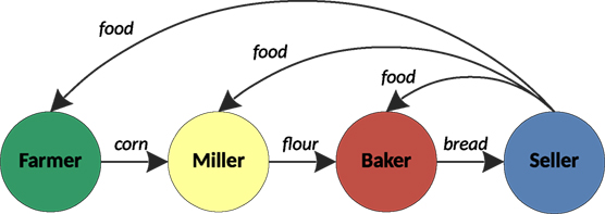
Figure 1. Food production cycle and dependencies between entrepreneurs of different types.

In a multi-agent population, the dependencies highlighted in Figure 1 create a complex network of mutual relationships between individual entrepreneurs where each producer:

• decides autonomously and independently when and with whom they establish a business relationship, how long they maintain it, negotiates with others for sale/purchase prices, etc.,

• knows the position of other individuals, but can interact only with those who are in a certain neighborhood,

• can move in the environment to find a neighborhood that is promising from a business perspective.

Moreover, ingredient production by each entrepreneur requires some time and energy (provided that necessary resources are available) in the following manner:

• Time requirement: each ingredient has its own amount of time to be produced. In order to reflect real conditions, the corn production is assumed to last longest in comparison to the other products, whereas production of other goods (flour, bread, food) is shorter.

• Energy consumption: is reflected by the vital energy of the producer that decreases over time. In order to replenish it, each individual must consume some food within a time, otherwise they will not survive. Figure 2 illustrates such a process.

FIGURE 2

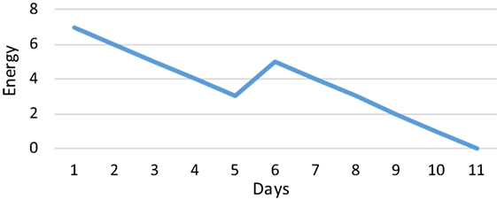
Figure 2. Example of the energy consumption over time. It can be noticed that on the 5th day some food was delivered and thereby the vital energy increased.

The above constraints make an entrepreneur act and make decisions (e.g., purchase, sale, and price negotiations) under time pressure. It means that such decisions can be non-optimal in the general sense; but even enforced, can be also unprofitable at a given moment.

All the above entails that producers start to compete with each other and contest for selling their goods, some of them can offer lower prices than others, or preferential rates for regular customers, gain the market, and even eliminate other competitors. In other words, a network of economic relationships between individual producers constantly and dynamically changes over time.

3. High-Level Model of the Multi-Agent System for Economic Relations (MASER)

A schematic MASER architecture is presented in Figure 3, where the following major components are emphasized:

• Environment

• Agent’s world

• Interactions between agents

• Relationships between agents.

FIGURE 3

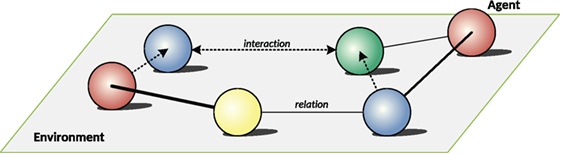
Figure 3. A schematic high-level MASER architecture.

3.1. MASER Environment

For MASER purposes, the Environment provides not only a space where agents can move and interact with each other but also some global functionalities that make agents exist and operate. In particular, the Environment is used for the following purposes:

• provide a 2D finite space (rectangular map) in which each agent has its size occupying some space, can move and can interact with its neighbors, which is illustrated in Figure 4,

• store each agent, especially their positions in the space,

• control agents’ movement, so that they do not collide or occupy the same space,

• identifies neighbors of a given agent.

FIGURE 4

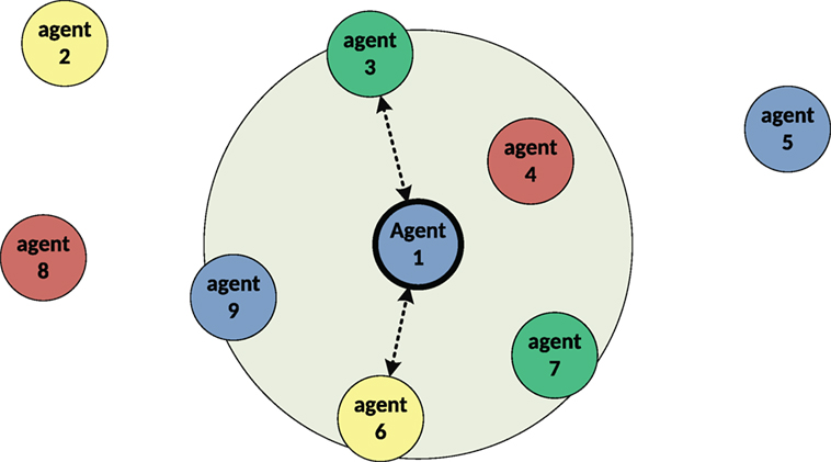
Figure 4. Example of the Environment with some agents and the neighborhood for Agent 1.

3.2. MASER Agent’s World

There are two fundamental Agent goals that drive its decisions:

• maximize their profit.

• provide for supplies (food) essential to replenish energy.

This is why any producer negotiates with others to purchase food and resources at the lowest prices, and to sell goods at the highest ones (from their perspective). In turn, their decisions are derivatives of the Agent world that is actually based on its properties and behaviors.

3.2.1. Properties

From a number of various properties, the following ones are of the most importance:

• Agent type: identifies if the Agent is a Farmer, Miller, Baker, or Seller.

• Production time: time in (virtual) days needed to produce goods.

• Velocity: speed at which the Agent moves in the environment. It affects the stability of interactions and relations between agents: a big value means the Agent can interact with many new ones and lose contacts quickly, whereas a small value means the Agent can have stable relations with others.

• Neighborhood radius: determines the range within which the Agent can interact with others. In the extreme case, the range can cover the whole environment space, whereas a too small radius leads to few interactions, if any. It helps in drawing up a list of neighboring agents, which changes over time as the Agent moves in the Environment.

• Budget: amount of money at Agent disposal that can be used for purchases of food or resources for production.

• Commodities: collection of resources for production, goods produced, and purchased food.

• Transaction history: list of transactions over time; used in business relations (for example) when offering prices to regular customers.

• Risk factor: inclination to take a risk, determines if the Agent is more like a risk-taker, or moderate. The greater the value is, the entrepreneur is more prone to raise prices, to ignore lacking food, and not to offer preferential rates for regular customers. In turn, a lower value makes the Agent establish a steady cooperation, and stock up on food.

• Package size: amount of food in one package that thereby defines the granularity of all food transactions. In other words, food is bought or sold in number-of-packages units.

• Advertising factor: probability of resetting the list of those agents that have already got an advertisement from the Agent (in every production cycle). Each entrepreneur needs to advertise, so that others know their offer. The factor prevents sending of spam.

3.2.2. Behaviors

Agent operation capabilities are determined by the following set of behaviors that can be demonstrated each virtual day:

• Movement

• Purchase (decision and transaction)

• Production

• Making an offer

• Sale (transaction)

• Food intake.

Their descriptions are provided further in the section, and Figure 5 gives an illustration to show if a given behavior is internal or is a kind of interaction with others (agents or the Environment).

FIGURE 5

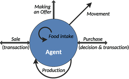
Figure 5. Agent behaviors. Arrows indicate the direction of action or interaction.

3.2.2.1. Movement

The goal of the movement behavior is to increase the business prospect of the Agent by means of finding such a place in the Environment where the Agent has real or potential business partners in its neighborhood. The result is a motion vector toward the place (the null vector corresponds to no movement).

The behavior is a three-phase decision system (see Appendix S1 in Supplementary Material for formal details):

• Business prospect assessment: evaluation if the current neighborhood is satisfactory based on what other agents are neighbors (food and resources sellers, and customers of Agent goods). The satisfaction is also dependent on the Agent risk factor, i.e., the more Agent is a risk-taker, the less satisfied it is (and tends to find another better place).

• Movement type decision: if the business prospect is satisfactory then the Agents attempts to retain the neighborhood (stops or stays in the place), otherwise it looks for a new opportunity (keeps moving or moves from the place).

• Movement direction and speed decision: if the decision is to be in motion (move or keep moving), then the Agent decides which direction is the most promising by means of taking into account positions of other agents in the Environment and the history of transaction between the Agent and them. Once the direction is determined, the final speed is calculated. An illustration of the decision is shown in Figure 6.

FIGURE 6

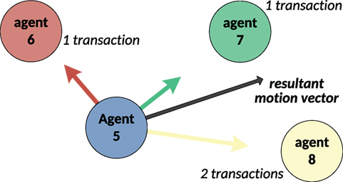
Figure 6. Example of a motion vector as the resultant one of vectors toward other agents, where transaction history is taken into account. Agent 5 had one transaction with agent 6 and 7 and two with agent 8 (longer vector toward agent 8).

3.2.2.2. Purchase (Decision)

The goal of the purchase behavior is to determine if the offer is affordable or necessary to the Agent, and its price can be accepted by taking into account the current amount of provisions.

Rules applied in the behavior are rather the same regardless of whether food or resources are concerned. In a general case, this is a sequence of IF-clauses as below (see Appendix S2 in Supplementary Material for more details):

• If the offer is not interesting: which means this is not the food or resources needed for production by the Agent (dependent on its type), then the decision is: not to purchase. Otherwise (might be interesting offer) the next IF-clause is applied.

• If the Agent cannot afford the offer: in other words, the Agent does not have a budget for it, so the decision is: not to purchase. Otherwise (can afford the offer), the flow goes to the next IF-clause.

• If this is the first Agent transaction: so the Agent does not have any knowledge about prices and their history, then the decision is: purchase. Otherwise information on the last prices (taken from the history of transactions) becomes essential, and the next IF-clause is fired.

• If this is a bargain: i.e., the offered price is not higher than the previous one, then the decision is: purchase. Otherwise some risk assessment needs to be done in terms of: to buy the expensive goods at this moment, or not to buy with respect to the current stock of food/resources. In consequence, the next IF-clause is employed.

• If the Agent can take a risk: which happens in the case of less restrained agents, then the decision is: not to purchase. Otherwise, the Agent decides to accept the offer.

3.2.2.3. Purchase (Transaction)

The objective of the Purchase behavior is to finalize the transaction of buying goods by the Agent at the negotiated price with another one (seller).

As a result, the Agent stock is replenished with some goods (purchased resources or food), whereas a respective payment is transferred to the seller agent. This transaction is then coupled with the Sale (transaction) of another agent. The behavior is formally presented in Appendix S3 in Supplementary Material.

3.2.2.4. Production

The purpose of the Production behavior is to produce goods from resources available to the Agent at the lowest cost.

The behavior is composed of the following steps (see Appendix S4 in Supplementary Material for formal information):

• Resources determination: determines if the Agent has any resources available for production. If not, there will be no production in a given production cycle.

• Production: takes resources in the Agent stock and produces goods according to the Agent specialization (as is described in Chapter 3). The resources are used in the ascending order of prices (the cheapest first) to have the lowest production costs, which translates to attractive goods prices in the case when resources were bought at different costs. This approach increases the Agent’s chances, because such goods can be sold fast. The production takes an amount of time when the Agent consumes energy.

• Cost calculation: calculates production costs of the goods, taking into account the purchase prices of resources used.

3.2.2.5. Making an Offer

The goal of the Making an Offer behavior is to decide whether to make an offer to a given potential customer, and if they decide so – what price to propose. The proposed price to different agents usually varies.

In the behavior, the following elements can be distinguished (see Appendix S5 in Supplementary Material for more details):

• Make-offer decision: decides if the Agent will make an offer to a given neighboring agent. In general, the Agent remembers if it has sent an offer, so it should not do the same twice to spam others, especially as handling messages costs some time. However, the Agent should be able to repeat its attempt to make a transaction because the business environment has changed (e.g., prices), and another agent may accept a new proposal. So, if there has been no offer to a given agent so far, then such a one will be made. Otherwise, the Agent clears (with a certain probability) its memory regarding to whom it has already sent an offer. As a result, the Agent will resend its most recent offer to individuals in the neighborhood.

• Offer price calculation: in a few steps calculates the offer price. First, sets the minimal price that returns the production and selling costs. Next, the price is increased by a retail margin that is calculated by taking into account if the Agent is a risk taker (greater margin) or not, and if the offeree is a regular customer. If this is the first contact between the agents, the increased price becomes the final one, because there is no business experience. Otherwise, the price is additionally adjusted for further negotiations dependently on: if the Agent’s offer was already rejected or accepted, if the current price is greater or lower than the one offered previously, how much the Agent is prone to risk-taking, and the amount of food at Agent disposal.

• Sending offer: sends the offer (price for the goods) to the neighboring agent.

After having sent the offer, the Agent can make an offer to another agent in its neighborhood.

3.2.2.6. Sale (Transaction)

The objective of the sale (transaction) behavior is to finally sell goods at the negotiated price to the agent (customer) that accepted the highest price (and thereby ensures the best profit) in a given period of time (one day).

The behavior is composed of the following simple IF-clauses:

• If no goods in stock: first, the Agent double checks if it has still goods in stock. If not, i.e., it has sold it out in the meanwhile, it refuses the transaction (and quits).

• If one customer: only one offer was accepted, so the Agent sells goods to a given agent.

• If many customers: the Agent compares the prices negotiated with agents that accepted them, and next chooses the one that agreed to the highest prices.

At the end of the transaction, some respective amount of money is added to the Agent budget, whereas the stock of another agent is replenished with the goods accordingly. This is why the behavior is coupled with the purchase (transaction) behavior of another agent. Some formal details of the behavior are given in Appendix S6 in Supplementary Material.

3.2.2.7. Food Intake

The Food Intake behavior reflects expenses of the Agent existence, i.e., Agent activities cost some energy that be replenished by means of food consumption. It means also that the Agent operates under time pressure, i.e., it needs to make a decision, even far from optimal, otherwise it would not have energy for existence.

The behavior consists in consuming, by the Agent, a fixed portion of food on a daily basis, and its simple formalism can be found in Appendix S7 in Supplementary Material.

3.2.3. Example of Agent Activities over Time

In order to illustrate the model of the Agent world presented in the preceding sections, one can use the following example. Let the k-th day together with the preceding- and following ones be considered (Figure 7).

FIGURE 7

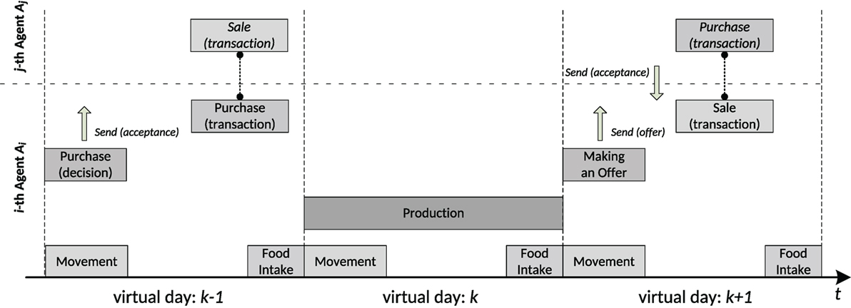
Figure 7. Example of Agent activities over time.

On the preceding day (k − 1), the i-th Agent is moving to find a proper business neighborhood (Movement behavior) and is also making a decision on buying necessary resources for production (Purchase decision). Once the decision is made (the Agent agrees on the price proposed), it sends a respective message regarding the offer acceptance. As soon as another agent (the j-th one) gets the information, it initiates a selling operation on its side (Sale transaction) that is coupled with the Agent behavior accountable for buying (Purchase transaction). The transaction makes the resources, and money are transferred between the agents. At the end of the preceding day, the Agent is consuming some fixed amount of food to replenish the energy loss (Food Intake).

On the next k-th day, the Agent decides to keep moving (Movement) and because it has enough resources for production, it starts the production of goods specific to its type, e.g., flour (Production). In the case of the Agent, the production lasts one day, and at the end of the day, it consumes some food, as usually (Food Intake).

On the following day (k + 1), the Agent makes a decision as regards its next move (movement) and can, for example, decide to stop moving, because of an attractive business neighborhood. As soon as the Agent has produced goods, it advertises the goods to neighboring agents (Making an Offer) by sending them an offer. If at least one agent accepts the offer, it sends a respective acceptance. As the Agent gets the message with the acceptance of its offer, it decides to sell the j-th agent the goods, and next is making a purchase-sale operation (Sale transaction). As a result the goods are shipped to another agent, whereas a corresponding amount of money is transferred to the Agent. The Agent is also replenishing its energy loss (Food Intake).

It is worth noting that Movement and Food Intake are the Agent’s permanent behaviors in the sense that they occur every day regardless of other triggers.

3.3. Interaction between Agents

Interactions between agents and in consequence transferring goods, money, and building up respective relationships are based on communication between them that encompasses both messages sent and transaction protocols.

3.3.1. Communication and Messages

In order to support communication between agents, each of them has the following features:

• is equipped with a Mailbox where incoming messages are stored.

• capability to receive (and read) messages from the Mailbox.

• capability to build up messages and send them to another agent or agents.

The format of a single message is composed of a number of fields, from which the following ones are most important from the functional perspective:

• Addressee and Sender: agent to which the message is addressed or that sends the message.

• Type: information if the message is an Offer, or it is an Answer (acceptance or rejection) to the offer already made.

• Body: describes the context of the message, especially in terms of type of goods (what resources, products and food), their quantity and price. Dependently on the type of the message, the field conveys the information as below:

• Type = Offer: goods and their quantity the Agent offers together with their prices adjusted to a given agent (addressee).

• Type = Answer: product and quantity the Agent decided to purchase or information about the offer rejection.

3.3.2. Transactions Protocol

Negotiations between agents, especially fixing a price, requires a certain protocol that is based on communication as: Send (offer) ↔ Send (answer).

An example of a protocol for 2-step negotiations is shown in Table 1. Agent A_i is a producer, and having once prepared a price proposal for its goods for agent A_j (customer), is sending an offer to it. The offer price is not attractive to the customer A_j that is sending an answer with its rejection. Next, the producer A_i is modifying its price proposal, and is sending an updated offer to the customer. This time the second proposal is acceptable to agent A_j that is sending its acceptance. If only the producer has still the goods in stock (it might have already sold them out as the negotiations take time), it is selling them in an atomic operation: at the same time, the goods are shipped to A_j, whereas money is transferred to A_i.

TABLE 1

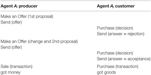
Table 1. Example of a protocol for a 2-step negotiations.

3.4. Building-up Relationships between Agents

It is assumed that relationships between agents are built up by means of a regular-customer policy that affects fixing prices (for a given agent) and in consequence the level of an individual transaction. It means the policy promotes some agents that get offers at more preferential prices than others. Thanks to lowered prices, more transactions (mutually advantageous) between respective agents are expected, which can lead to tightening business relationships.

From a quantitative perspective, the policy is implemented with the help of the Agent behavior and looks as follows whereas some formalism can be found in Appendix S8 in Supplementary Material:

• each agent has a list of its customers and grants a number of points.

• the more points a given agent has the more promoted it is (especially during the fixing of prices).

• at each transaction, the number of points granted to the customer by the Agent is increased by the level of the transaction.

• every day if there is no transaction between the two agents, the customer points are decreased dependently on the average value of transactions between them, the average time between transactions, and Agent’s inclination to take a risk.

3.5. Time Analysis of Agent Activities and Interactions

Agent behaviors have a determined duration time in the following way:

• explicitly and precisely: the production time is defined as per agent type and is expressed in units of virtual days (as the agent property)

• inexplicitly: behaviors that need to be completed within a virtual day (see section 3.2.3)

In turn, communication in terms of message handling time or the duration of interactions (e.g., negotiations or transactions) are unpredictable; due to their stochastic nature, their values are instantaneous and depend mainly on neighboring and interacting agents at a given moment, intensity of communications, offers proposed by negotiating agents, etc. This section provides a sort of time analysis of agent behaviors and interactions that includes two perspectives: the agent’s one, and the second one for the food production cycle.

3.5.1. Time Dependencies from the Agent’s Perspective

From the perspective of an individual agent, time dependencies comprise all activities (behaviors, communication, interactions) over some time that is needed to buy food, or to purchase resources for production and the production itself. In other words, two components contribute to the period: a fixed production time T^ω and an unpredictable lead time Δt^ω used for interactions and communication.

Figure 8 illustrates the case assuming T^ω = 1 (day) and the following three scenarios:

• Case (A): the Agent has enough resources in stock to start the production, which gives no lead time (Δt^ω = 0), i.e., the Agent triggers the production at once. Although in parallel, it can start seeking sellers of resources, negotiate prices, etc., however, they are not critical for the current production, so the next day, the product can be offered by the Agent.

• Case (B): the Agent has not enough resources, however got an offer from another agent, accepted it, and the transaction was finalized on the same day. It cannot already start the production, but does it next day, so the lead day T^ω is equal to 1 day. Once the Agent produces a product, it begins negotiations to sell it, but it takes place in 2 days in total.

• Case (C): the Agent also has not the necessary quantity for production, but additionally, it is involved in heavy correspondence, which means that not all messages are read on the same day. In consequence, a negotiation is finalized not until the next day. This is why the production can start in 2 days.

FIGURE 8

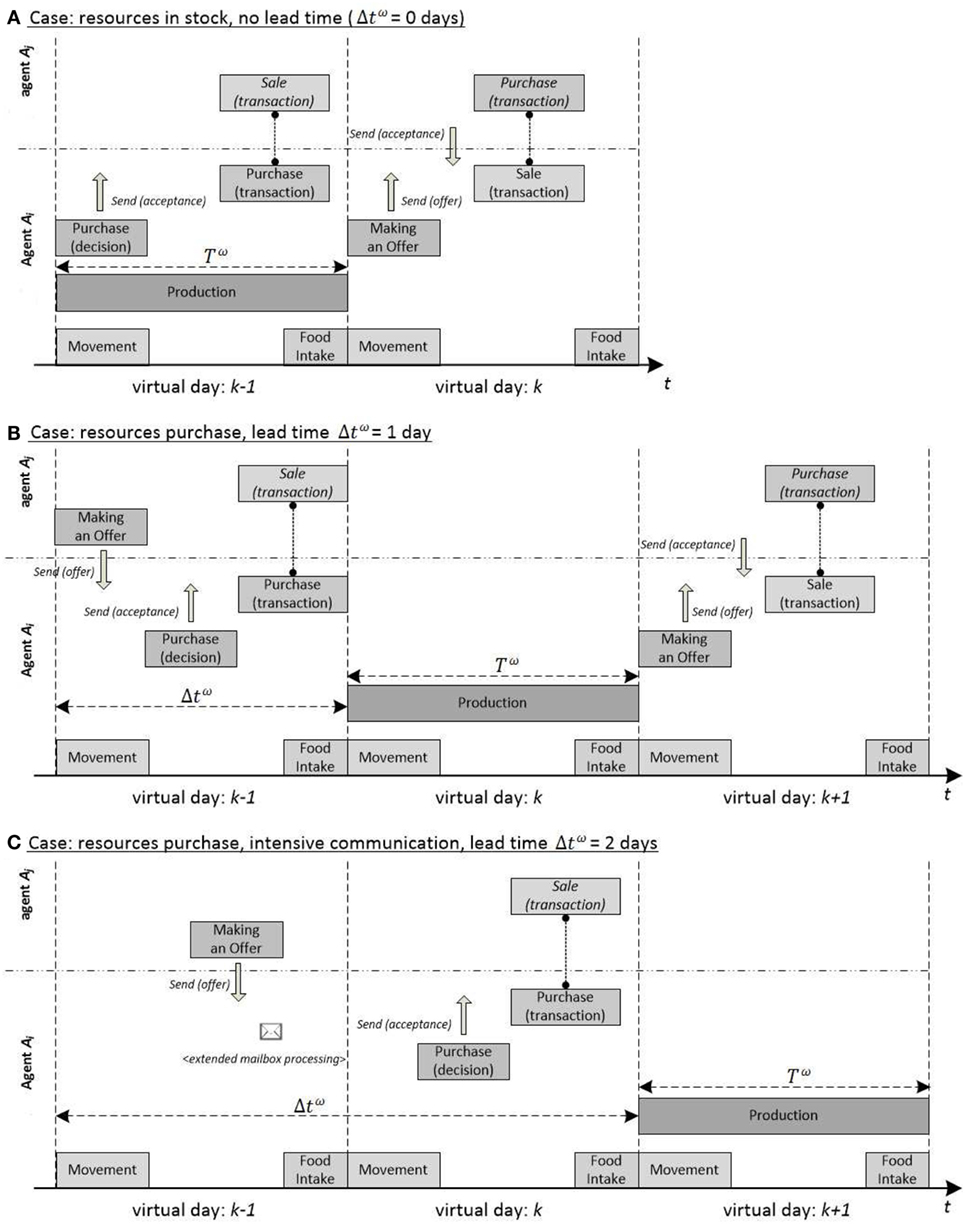
Figure 8. Time dependencies from the agent’s perspective.

3.5.2. Time Dependencies between Agents in the Production Cycle

The perspective of the food production cycle (presented in Section 2) refers to the time needed to go through the whole cycle (incl. production times and communications/interactions) to produce and get food, i.e., how much time passes from when a given agent produces goods until they purchase food made from that agent’s ingredient. Due to an unpredictable lead time, T^ω reflecting interaction/communication between agents such dependencies can be illustrated only using some assumptions. A simplified example is depicted in Figure 9 where the production time T^ω (day) for all agents, each of them needs exactly 1 day for selling goods and buying resources (lead time T^ω = 1, case (B) in Figure 8). In such a case, the Farmer needs 7 days to purchase food produced from its ingredients (corn), whereas the Miller, Baker, and Seller get food in 5, 3, and 1 virtual days, respectively.

FIGURE 9

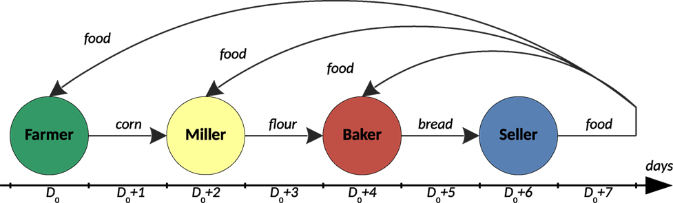
Figure 9. Example of simplified time dependencies between entrepreneurs of different types during one food production cycle that starts on day D₀.

4. Simulations

4.1. Environment for Simulations

For simulation purposes, the Multi-Agent System for Economic Relations (MASER) was implemented from scratch in the C# programing language and with the use of .NET and MVC (Model-View-Controller) technology. Each agent is implemented in a separate thread to provide it with autonomy and to reflect its internal independent world.

In experiments, the MASER user interface reflects the concept illustrated in Figure 3, and each agent is represented by a circle whose color indicates its type in the way as is shown in Figure 10.

FIGURE 10

Figure 10. Representation of agent types in MASER.

4.2. Initial Conditions for a Single Simulation

At the start a number of agents of each type (i.e., Farmers, Millers, Bakers, Sellers) is created, and randomly distributed in the 2D Environment, i.e., in a rectangle of a given size. For these types, respective production times are set, and remain fixed during a simulation.

Each agent gets the risk factor set randomly, which makes all of them behave differently, especially in terms of negotiations and making decisions. In addition, all agents get the same neighborhood range (radius) in which business transactions can occur.

At the beginning, agents have no goods, no relationships, they get only some budget and “free” food that are supposed to be sufficient, until they find business partners for: buying food and necessary resources for production, and selling produced goods to earn money for further purchases. Initially, the food price is also determined, and used only in first production cycles to prevent Sellers from profiteering from the “free” food. Just in a simulation, they need to create the full production cycle (Figure 1). So, for every simulation, the following MASER parameters need to be set:

• number of agents of each type

• production times (per each agent type)

• initial budget (equally distributed)

• initial free’ food (equally distributed)

• food price at start

• risk factor (range of random values)

• neighborhood radius

• size of the 2D Environment.

4.3. Examples of Simulation Results

A number of various simulations were executed from the following different perspectives:

• Experiment #1: average goods prices in time

• Experiment #2: various arrangements of agents in 2D

• Experiment #3: evolution in time of 2D agents’s arrangements

• case: stable agent relationships and arrangements in time

• case: decay of relationships leading to extinction

• Experiment #4: rearrangements of a 2D agent population in time

• Experiment #5: dynamics of relations between agents in time.

4.3.1. Experiment #1: Average Goods Prices in Time

The goal of the experiment was to observe how some basic economic parameters such as: average prices of goods and average prices fixed during transactions change over time.

An example of some preliminary simulations is presented in Figure 11 (initial conditions are shown in Table 2), where two types of average prices that are current on a given day are placed:

• Prices offered by all agents producing goods of the same type are taken into account. This means that even if an agent is not selling anything at a particular moment, the current price of its goods is the same as the one from its last transaction.

• Only prices of transactions regarding the same goods, and concluded on that day, contribute to the average.

FIGURE 11

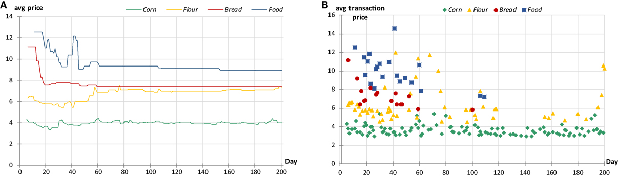
Figure 11. Example of average goods prices in time: (A) Average prices offered and (B) average prices of realized transactions.

TABLE 2

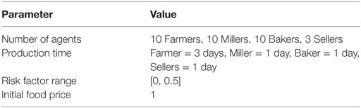
Table 2. Initial conditions for experiment #1.

After some strong fluctuations at the beginning (partially due to initial conditions), the average prices get mid-term stabilization. On the other hand, the number of transactions lowers, especially those referring to food sales. It can mean that individual agents may have enough food in stock, so they do not need to buy it more. However, it is worth noticing that corn-related transactions are rather at the same rate. Figure 11 shows also how margins affect prices: the distance between respective curves reflects to a certain extent the mark-ups surcharged by agents. An interesting case is as the average flour prices get very close to those of bread. The chart (B) suggests that some initial transactions at an overvalue influence subsequent ones. It can also be noticed that transactions, and thereby fixing prices, begin after a few days, and their starting points are shifted with respect to each other. This reflects time dependencies in the production cycle between agents producing different goods as is described in Section 3.5.2.

4.3.2. Experiment #2: Various Arrangements of Agents in 2D

The goal of the experiment was to observe various spatial arrangements of agent populations in which bonds between agents are determined by their mutual economic relationships. It is worth noting that the relationships are always short term, change over time, and thereby are vulnerable to instability in time.

Initial conditions for the experiment are collected in Table 3. In many simulations, one could observe different conglomerates of agents that looked like chaotic or disorderly spatial arrangements. One could also discover more organized structures that formed during the evolution of populations in time, and such results are presented in Figure 12 where one can find three visually interesting arrangements:

• Case (A): although the arrangement suggests one cluster of agents, there are largely two groups localized around Sellers (in blue). In addition, some agents between them (e.g., Miller 15, Baker 25) can cooperate with the two subgroups. On the basis of such types of configurations, quite stable arrangements can form, because in the neighborhood of agents, there are various types of individuals that can ensure the production cycle (see Figure 1).

• Case (B): the grouping of agents around the central Seller 31 seems to be stable, whereas subgroups around the outermost Sellers 32 and 33 are exposed to a change of their arrangements due to a small number of agents of necessary types that would provide and sustain the food production cycle (Figure 1). Then, one can expect some reconfigurations on the edges that can make the stability around Seller 31 mid-term due to the interaction of competing agents from the subgroups around Sellers 32 and 33.

• Case (C): two groupings around Sellers 31 and 32 that are separated from one another are formed, where business transactions are taking place within these groups. They seem to be quite stable, although more vulnerable to a change is the subgroup around Seller 31, because not all agents there have “necessary” neighbors in a safe distance (e.g., Farmer 4 or Baker 30). In the case of a small movement, for example partners move outside the neighborhood range, and potential transactions would not be possible between respective agents, which enforces some further moves, and thereby a reconfiguration.

TABLE 3

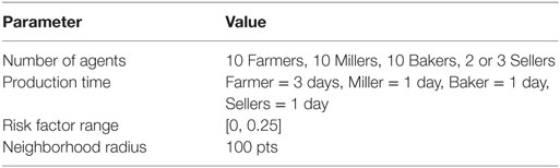
Table 3. Initial conditions for experiment #2.

FIGURE 12

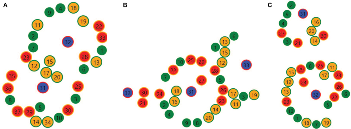
Figure 12. Example of various agent arrangements in the 2D space: (A) One cluster composing of two adjacent groups, (B) stable central structure with impermanent neighboring groups, and (C) stable separated clusters.

4.3.3. Experiment #3: Evolution in Time of Agent Arrangements

The goal of the experiment was to observe the behavior of agent populations over time in terms of how their arrangements evolve, if and why they form stable configurations or decay.

4.3.3.1. Case A: Stable Agent Relationships and Arrangements in Time

An example of a successful evolution of an agent population in terms of a final stable spatial configuration is presented in Figure 13 (for initial conditions as in Table 4). It is worth noting that a necessary condition (but not sufficient) of stability is: within the neighborhood radius there must be agents that can provide resources for production, can become receivers of produced goods (see Table S2 in Supplementary Material) and can sell food.

FIGURE 13

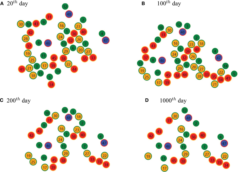
Figure 13. Example of stable agent arrangements in time: (A) On the 20th day, (B) on the 100th day, (C) on the 200th day, and (D) on the 1000th day.

TABLE 4

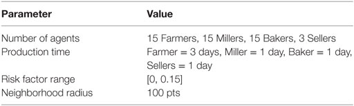
Table 4. Initial conditions for experiment #3, case A.

From an initial population of agents randomly dispersed in the 2D space, the first cluster of agents emerges on day 20, which assumes a quite stable form between day 100 and day 200. For the next 800 days, this arrangement (or, in other words, economic ecosystem) remains long-lasting with slight changes. The reasons of such durable stability one can find in a pretty good distribution of agents (i.e., sufficient number of agents of necessary types as neighbors), as well as in the relatively small risk factor that makes agents less prone to look for new positions and more careful in negotiations.

4.3.3.2. Case B: Decay of Relationships Leading to Extinction of Agents

Populations of agents can also become extinct due to the decay of economic relationships between them, and an example of such a situation for the initial condition as in Table 5 is shown in Figure 14.

TABLE 5

Table 5. Initial conditions for experiment #3, case B.

FIGURE 14

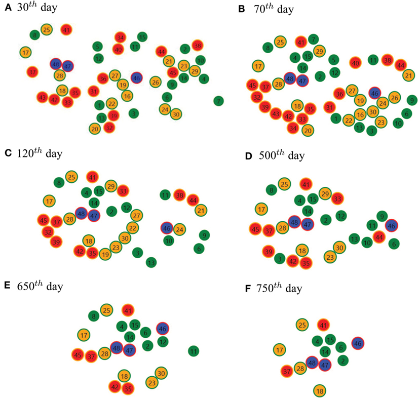
Figure 14. Example of an agent population decaying in time: (A) On the 30th day, (B) on the 70th day, (C) on the 120th day, (D) on the 500th day, (E) on the 650th day, and (F) on the 750th day.

From an initial disorderly (i.e., randomly distributed) population of agents, there begins a consolidation of individuals (day 30), and next, on day 70 a configuration emerges that seems to be stable. The shaping lasts for dozens of days until day 120, and then, for a quite long time (till day 500), the arrangements get stabilized in terms of the balanced distribution of agents, i.e., their diversity. On day 120, one can observe groupings of Bakers or Millers, whereas on day 500 their distribution is more diverse. Next, bonds between agents gradually decay until they are extinct. On day 750, one can still observe all types of agents. A direct cause is obvious, the chain of the food production cycle gets broken, i.e., at least one type of agents vanishes. But the reason why it happens is more complicated. A high value of the risk factor that is taken into account in decision systems (incl. negotiations) seems to be the likely reason. Especially as agents are able then to prolong negotiations and break them off suddenly, because they take more risk and count on the next opportunity that can be more profitable. In consequence such agents are prone to more frequent moves.

The way how the risk factor affects agent movement is illustrated in Figure 15 where movements of agents of all types in the 2D space are depicted. Labels near to data points represent consecutive (virtual) days, and color lines indicate the path traveled by an agent of a given type. In the case of a lower risk factor movements are steady, agents tend to some targets, and when they reach them, they rather stay there. In turn, as the risk factor is greater, agents seem to be in rather permanent movement, as if they were constantly looking for new opportunities.

FIGURE 15

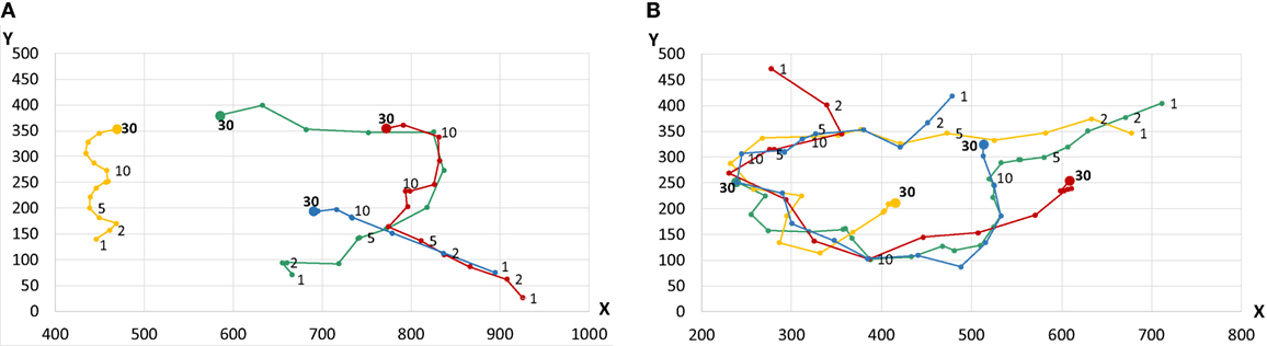
Figure 15. Example of the influence of the risk on affects movement of agents: (A) Risk factor = 0.15, (B) risk factor = 0.5, where the average path traveled by an agent in 1 day is 17.17, and 30.38, respectively.

4.3.4. Experiment #4: Rearrangements of an Agent Population in Time

The goal of the experiment was to observe how a population of agents behaves when, after a spatial arrangement has been created, a key agent gets removed from it and is placed in another spot in the Environment. An example of rearranging agents spatially under such a scenario and for initial conditions as in Table 6 is demonstrated in Figure 16.

TABLE 6

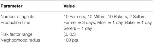
Table 6. Initial conditions for experiment #4.

FIGURE 16

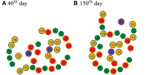
Figure 16. Example of a change of agents arrangement in time: (A) On the 40th day, (B) on the 150th day.

It can be observed that on day 40 the population of agents tends to form an arrangement resembling an ellipse whose foci are Seller 31 and 32. On the same day, agent 32 gets shifted to another spot in the 2D space. After more than 100 days (on day 150), the population has rearranged, and the central part is a circular arrangement around Seller 31, whereas Seller 32 is flanked by agents of various types (in other words, the Seller may provide them with some food). The reason for the rearrangement lies in the mobility of agents. If a key agent that has business transactions with many other individuals gets moved far away, the other agents lose their current relations, so they start looking for new opportunities and move toward the substitute (Seller 32).

4.3.5. Experiment #5: Dynamics of Relations between Agents in Time

The goal of the experiment was to observe how relations between agents (in terms of transactions between them) change over time in a population of parameters presented in Table 7. In turn, an example of the relation dynamics is illustrated in Figures 17 and 18.

TABLE 7

Table 7. Initial conditions for experiment #5.

FIGURE 17

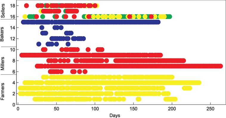
Figure 17. Example of transactions between agents in time. Each circle represents one transaction. The positions of the circles correspond to days and the type of agents selling goods. The colors of the circles represent the types of agents buying goods as follows: green represents Farmers, yellow – Millers, red – Bakers, and blue – Sellers.

FIGURE 18

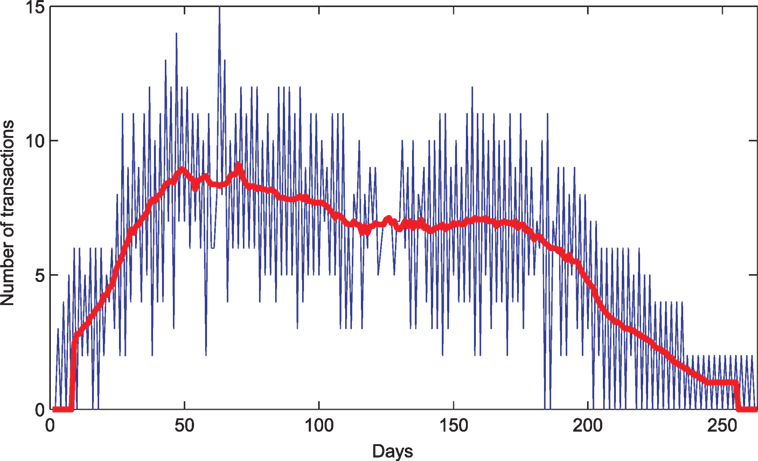
Figure 18. Total number of transactions between agents in days. The thick line represents the moving average with the window size equal to 16.

At the beginning of the simulation one can notice a transient phase with a growing number of transactions between various agents. It is caused by moving agents in search of contacts for buying/selling purposes, which find partners, set up relations and make transactions. Over time (around day 70), the relations get stabilized to a certain extent and last for some time (till day 180). The number of transactions lowers, however they are made between same agents more often than between new ones. That might suggest more stable relations than at the beginning. Such a situation is very likely caused by the fact that agents have finally found favorable business conditions (in their neighborhoods), which made possible to establish more durable relationships.

5. Conclusion

The presented MASER model combines mutual economic dependencies between agents as closed-loops with complexity of agents’ behavior (algorithmic decision systems). A number of agents of four types occupy a two-dimensional space. In order to live, agents have to eat food. In order to eat, they have to purchase resources, produce goods, sell them, and buy food for earned money. In order to do that, they have to find potential contractors in their vicinity, negotiate the prices of goods, and then create business relations for exchanging goods. The created relations are only for single portions of goods so they last for a limited time only so they are constantly changing, breaking, and creating a new possibility with another partner. Moreover, to keep the situation stable the relations between agents must form a closed loop.

Basically, closed-loops are employed in the field of ecosystems modeling (e.g., Lotka–Volterra equations) or chemical kinetics (e.g., Belousov–Zhabotinsky reaction or brusselator), and their dynamics can be described by differential equations. As was discusses in Introduction, there are classes of real closed-loops systems (e.g., economics), where complexity of interactions between their elements makes the system dynamics impossible to be described using a traditional mathematical approach. And the same case is for the MASER model, in which relations between agents and their behaviors are the results of complicated algorithms, incl. negotiations or other decision rules, and keeping closed-loop ones is a condition of the agent activity. Such relations can change over time, sometimes they can lead to short-term quasi-stable equilibria between interacting agents, and are also extremely vulnerable to parameter values and their changes. In a consequence, all the above make the system exceptionally complex and practically indescribable by means of analytical tools, so knowledge of its evolution in time can be obtained only by computer simulations. Last but not least, this closed-loop aspect is hardly met and discussed in MAS-related literature.

The second part of the paper presents the results of a few preliminary simulations, in which an experimental focus is put on emergence of self-organizing patterns. The results show the tendency of agents to self-organize by creating loops of relations. These relations are quasi-stable in the sense that the agents form spatial clusters in which the positions of agents only slightly change from time to time despite often changed relations, and these clusters last for longer periods of time. The other simulations showed that removing from such clusters an important agent, and shifting it to another place, thus breaking the vital loops, that spatial reconfiguration of agents occur resulting in organizing other clusters of loops.

Generally, the simulation showed the chaotic behavior of the system manifested by a strong sensitivity to applied parameters. For example, setting very small or large risk factors of agents leads unexpectedly to progressive extinction of the agent population.

Even preliminary MASER simulations provide some interesting observations as short- and medium-term equilibria of economic relations that are manifested by both stabilization of economic parameters (e.g., average prices) and spatial layouts of agents. They also give insight into the directions of further research and simulation experiments. The first group of simulations will contain the research on the influence of various parameters of the agents on the stability of the system manifested by the average duration of life of the agents. It will also try to classify the time evolution of the system into a few typical patterns depending on the settings of the parameters. The second group will be using the machine-learning approach to optimize the behavior of the agents to obtain a system maximally stable. It will be important to see to what degree the greediness of agents is limited to achieve such a global objective.

Another task will be tuning the parameters of the systems or even extending its rules to model the economic or social crisis situations leading to the forming of new spatial positions of agents and massive rearrangements its relations. An important extension of the system will be introducing mechanisms of adaptation of agents, basing on their personal history and on observations of other agents’ performance, which will be similar to particle swarm optimization methods.

Author Contributions

All authors listed, have made substantial, direct and intellectual contribution to the work, and approved it for publication.

Conflict of Interest Statement

The authors declare that the research was conducted in the absence of any commercial or financial relationships that could be construed as a potential conflict of interest.

The handling Editor declared a shared affiliation, though no other collaboration, with one of the authors (WJ) and states that the process nevertheless met the standards of a fair and objective review.

Supplementary Material

The Supplementary Material for this article can be found online at https://www.frontiersin.org/article/10.3389/frobt.2016.00041

References

Ashby, W. R. (1962). “Principles of the self-organizing system” in Principles of Self-Organization: Transactions of the University of Illinois Symposium, eds. V. F. Heinz and G. W. Zopf (London: Pergamon), 255–278.

Google Scholar

Banzhaf, W. (2009). “Self-organizing systems,” in Encyclopedia of Complexity and Systems Science, ed. R. A. Meyers (Berlin: Springer), 8040–8050.

Google Scholar

Bonabeau, E. (2002). Agent-based modeling: methods and techniques for simulating human systems. Proc. Natl. Acad. Sci. U.S.A. 99(Suppl. 3), 7280–7287. doi:10.1073/pnas.082080899

PubMed Abstract | CrossRef Full Text | Google Scholar

Cristelli, M., Pietronero, L., and Zaccaria, A. (2011). Critical overview of agent-based models for economics. ArXiv e-prints.

Google Scholar

Di Marzo Serugendo, G., Gleizes, M.-P., and Karageorgos, A. (2005). Self-organization in multi-agent systems. Knowl. Eng. Rev. 20, 165–189. doi:10.1017/S0269888905000494

CrossRef Full Text | Google Scholar

Dressler, F. (2008). A study of self-organization mechanisms in ad hoc and sensor networks. Comput. Commun. 31, 3018–3029. doi:10.1016/j.comcom.2008.02.001

CrossRef Full Text | Google Scholar

Eigen, M. (1971). Selforganization of matter and the evolution of biological macromolecules. Naturwissenschaften 58, 465–523. doi:10.1007/BF00623322

CrossRef Full Text | Google Scholar

Gorodetskii, V. (2012). Self-organization and multiagent systems: I. models of multiagent self-organization. J. Comput. Syst. Sci. Int. 51, 256–281. doi:10.1134/S106423071201008X

CrossRef Full Text | Google Scholar

Haken, H. (1978). Synergetics. Berlin: Springer.

Google Scholar

Helbing, D. (2012). “Agent-based modeling,” in Social Self-Organization. Agent-Based Simulations and Experiments to Study Emergent Social Behavior, ed. D. Helbing (Berlin: Springer), 25–70.

Google Scholar

Heylighen, F., and Gershenson, C. (2003). The meaning of self-organization in computing. IEEE Intell. Syst. 18, 72–75. doi:10.1109/MIS.2003.1217631

CrossRef Full Text | Google Scholar

Holland, J. H., and Miller, J. H. (1991). Artificial adaptive agents in economic theory. Am. Econ. Rev. 81, 365–370.

Google Scholar

Johnston, J. (2008). The Allure of Machinic Life, Cybernetics, Artificial Life, and the New AI. A Bradford Book. Cambridge, MA: The MIT Press.

Google Scholar

Judd K. L. (2006). “Computationally intensive analyses in economics,” in Agent Based Computational Economics, Volume 2 of Handbook of Computational Economics, eds L. Tesfatsion and K. L. Judd (Amsterdam: Elsevier), 881–893.

Google Scholar

Nicolis, G., and Prigogine, I. (1977). Self-Organization in Nonequilibrium Systems: from Dissipative Structures to Order Through Fluctuations. New York: Wiley.

Google Scholar

Quesada, M., Amblard, F., Barcelo, J., and Madella, M. (eds) (2014). “Advances in computational social science and social simulation,” in Proceedings of 10th Artificial Economics Conference, Barcelona. Social Simulation Conference (Bellaterra, Cerdanyola del Valles).

Google Scholar

Railsback, S. F., Lytinen, S. L., and Jackson, S. K. (2006). Agent-based simulation platforms: review and development recommendations. Simulation 82, 609–623. doi:10.1177/0037549706073695

CrossRef Full Text | Google Scholar

Tesfatsion, L. (2003). Agent-based computational economics: modeling economies as complex adaptive systems. Inf. Sci. 149, 263–269. doi:10.1016/S0020-0255(02)00280-3

CrossRef Full Text | Google Scholar

Tesfatsion, L., and Judd, K. (eds) (2006). Agent Based Computational Economics. Number 2 in Handbook of Computational Economics. Amsterdam: Elsevier.

Google Scholar

Wolfram, S. (2002). A New Kind of Science. Champaign, IL: Wolfram Media Inc.

Google Scholar

Wooldridge, M. (2009). An Introduction to MultiAgent Systems. Chichester: Wiley.

Google Scholar