Morphological Modularity Can Enable the Evolution of Robot Behavior to Scale Linearly with the Number of Environmental Features

1. Introduction

Matarić and Cliff (1996) pointed out that the time necessary to evolve robots grows with the number of environments in which the robot should behave correctly. Following their work, let f be the number of free parameters in the environmental set and n_p be the number of features for each of these free parameters. So, the total number of environments is $n_p^f$. (For example, if a robot must behave appropriately in environments containing two objects (f = 2), and each object may be small, medium, or large (n_p = 3), then there are $n_p^f=3^2=9$ possible environments in which the robot must perform correctly.) Thus, in order to evolve robots to perform complex behavior (which means increasing n_p, f, or both) the number of environments the robot needs to be evolved in scales exponentially.

Pinville et al. (2011) presented one way to reduce the number of environments evaluated while still obtaining robust and generalized controllers for evolved robots. Using the ProGAb approach, they were able to successfully obtain robust and successful controllers with better generalization abilities in less time than other top methods. However, their work did neither look specifically at the structure of the controller and morphology as methods to reduce the necessary number of environments nor did it categorize which environments should be trained on.

The work presented here demonstrates that morphological and neural modularity is one possible way to reduce the number of environments needed for evolving robust behavior.

Modularity is ubiquitous at all levels of biological organization, from cells to distinct species. Explaining why such modularity exists, and how it evolved, remains an important question in biology. Much work has focused on how modularity evolves in non-embodied systems, but relatively little work has focused on the impact of modularity in evolving embodied systems. The work presented here contributes to this latter aim.

1.1. Non-Embodied Modularity

Wagner (1996) argued that a combination of directional and stabilizing selection, acting on different parts of the organism’s phenotype, should lead to modular developmental programs. Such modularity would enable evolutionary changes to that part of the phenotype experiencing directional selection while retaining the structure and function of the other parts of the phenotype under stabilizing selection.

This theoretical argument was confirmed by a number of computational experiments. Lipson et al. (2002) showed that environmental change can be a catalyst for the evolution of modularity. That work was followed by experiments in which non-embodied Boolean networks (Espinosa-Soto and Wagner, 2010) or neural networks (Kashtan and Alon, 2005; Clune et al., 2013) were evolved to perform various tasks. The tasks and fitness functions were chosen in such a way as to favor networks that computed partial results using separate genetic or neural modules; changes to the fitness function over evolutionary time favored networks that could rapidly change how those partial results were combined. Thus, stabilizing selection came to bear on the partial results, while directional selection acted on how those partial results were combined.

More recently, it has been shown that selecting sparse networks helps to favor the evolution of modular networks. Espinosa-Soto and Wagner (2010) accomplished this by formulating a biased mutation operator that favors low in-degree network nodes. Clune et al. (2013) used a multi-objective approach, in which one objective was to minimize the number of edges in the network. Bernatskiy and Bongard (2015) showed that this relationship between sparsity and modularity can be exploited to enhance the evolution of modular networks by seeding the initial population with sparse, rather than random, networks.

Modularity is a desirable property of artificial systems for a number of reasons, beyond just the desire to create biologically inspired artifacts. First, modular systems possess a form of robustness: modular systems can more rapidly adapt to certain kinds of changes in their environments, compared to non-modular systems. Second, modular neural networks are better able to avoid catastrophic forgetting than non-modular networks (Ellefsen et al., 2015). Catastrophic forgetting (French, 1999) is a common problem in machine learning, whereby a learner must forget something in order to learn something new. Third, complex predictive models and dense, non-modular networks can suffer from the pathology of overfitting: they fail to generalize to novel environments (Kouvaris et al., 2015). Modular networks can avoid overfitting by internally reflecting the modularity in its environment: it responds appropriately in a “new” environment, which is actually just an unfamiliar combination of familiar percepts.

1.2. Embodied Modularity

A modular robot may likewise be robust and avoid catastrophic forgetting and overfitting, but there are additional challenges that arise when evolving embodied agents compared to non-embodied networks and morphologies.

Embodied cognition is a particular approach to the understanding of intelligence, which holds that the body must necessarily be taken into any account of adaptive behavior (Brooks, 1990; Clark, 1998; Pfeifer and Bongard, 2006). One repercussion of the embodied cognitive stance is that if neural controllers are evolved for artificial embodied agents (i.e., robots), a given robot body plan may facilitate or hinder the evolution of desirable traits. In the context of modularity, previous work showed that there do exist body plans in which modular neural controllers will evolve (Bongard, 2011).

Follow-on work demonstrated that, given appropriate conditions, evolution will find such body plans (Bongard et al., 2015). However, in Bongard et al. (2015), the morphology itself was not modular, only the neural networks that evolved to control it.

Here, we investigate another aspect of the relationship between morphology and modularity: for a given task environment, must both the body and neural controller be modular, and if so, in what way? Before addressing these issues, however, we must define both neural modularity and morphological modularity.

1.3. Neural Modularity and Morphological Modularity

In this work, we investigate robots controlled by artificial neural networks. A common approach to measuring the amount of modularity in a network is to investigate its connectivity: a network that has dense connectivity within subsets of nodes, and relative sparsity between those subsets, is said to be modular (Newman, 2006). Following this approach, we here investigate modular neural controllers in which subsets of sensor, internal, and motor neurons are connected, but there are no synaptic connections between these subsets. We compare these to non-modular networks in which any sensor can influence any motor.

In a neural controller in which sensor information flows from sensor neurons to internal neurons to motor neurons, this structural approach to modularity implies a functional repercussion. If subsets of sensors and motors are completely structurally independent, they will be functionally independent as well: changes to a subset of sensors will only have an influence on a subset of motors.

Thus, we here define neural modularity in the following manner.

1.3.1. Neural Modularity

A neural network with i sensor neurons S = {s₁, s₂, …, s_i} and j motor neurons M = {m₁, m₂, …, m_j} is defined to be modular if every possible change to less than i of the sensors results in changes to less than j of the motors.

Conversely, in a non-modular neural controller, it is possible for a change to fewer than i sensors to influence the new values of all j motors. It is possible that a non-modular neural controller may internally extinguish certain sensor dynamics from reaching some motors, but we disregard this case in the present work. This results in a simplified, binary definition of modularity: either a neural controller is modular or not. Here, we investigate robots with both types of neural controller.

This approach to defining the modularity of robot neural controllers suggests a similar approach for defining the modularity of a robot’s body plan:

1.3.2. Morphological Modularity

A robot is defined to be morphologically modular if a change in less than j of its motors results in a change in the state of the world registered by at least one and strictly less than i of the robot’s sensors.

One common definition of morphology is any agent subsystem that mediates between its controller and its environment. More specifically, when an agent acts, it alters its relationship with its environment. If it is equipped with sensors, it can register this change. The above definition of morphological modularity captures the intuition that structural independence of the body, like structural independence of a neural network, implies functional independence: if a robot moves one part of its body that is independent of the rest of its body, local sensors will register the action, but more sensors on other morphological modules will not.

Armed with these two definitions, one can investigate four classes of robots:

1. those that are morphologically and neurally non-modular;

2. those that are morphologically modular but neurally non-modular;

3. those that are morphologically non-modular but neurally modular; or

4. those that are morphologically and neurally modular.

In this study, we evolve robots belonging to the first, second, and fourth class. One can deduce that robots which belong to the third class are functionally equivalent to those which belong to the first class: if a morphologically non-modular robot moves, its motion will affect all of its sensors. These sensors will then affect all motors, regardless of whether its neural controller is modular or not. Further, for this instance of the treebot, there is no design of a robot of the third class with a completely modular controller where both leaf sensors influence the motor neuron. If the controller was modular, only one or none of the leaf sensors would influence the motor neuron.

Although modular robots have been the focus of a number of studies (Yim et al., 2007; Fitch et al., 2014), here we compare morphologically modular and non-modular robots to investigate a specific and new question: if modular and non-modular robots are evolved in an increasing number of environments, are the robots with modular controllers able to detect familiar percepts combined in unfamiliar ways, and, with a modular morphology, respond appropriately?

This question brings to light a challenge for modular, embodied agents that modular, non-embodied systems do not experience. Even if an embodied agent has a modular neural controller with which it detects novel combinations of familiar percepts in a new environment, once it moves, its perceptions will change, and the environment may no longer “look” modular. We show here that movement in a new environment continues to appear modular from the robot’s point of view only if it also has a modular morphology: it is free to move in response to independent percepts as it did previously, without disrupting the sensory signals arriving at other morphological modules.

The methods employed for investigating this issue are described in the next section. Section 3 reports our results, while Sections 4 and 5 provide some analysis and concluding remarks, respectively.

2. Materials and Methods

This section describes the body plans of the simulated robots (Section 2.1), their various controllers (Section 2.2), the task environments they operated within (Section 2.3), the evolutionary algorithm used to optimize their controllers in those environments (Section 2.4), and the experimental design (Section 2.5).

2.1. The Robot Morphologies

Two robot morphologies were considered: one which is modular and one which is non-modular. Figures 1A,B represent robots with modular morphologies, while Figure 1C represents the non-modular one.

FIGURE 1

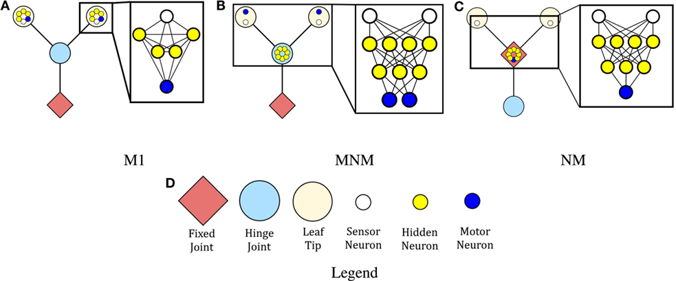
Figure 1. The controllers and morphologies for each of the three robots. The red diamonds indicate that branches connected at that position are fixed relative to one another. Large blue circles indicate that the branches rooted at the circles are free to move independently of one another. Beige circles represent leaf tips. The small circles represent neurons: blue neurons represent motor neurons, white neurons represent sensor neurons, and yellow neurons represent hidden neurons. The modular robot is represented by (A) on the left, the mod-non-modular (B) is in the middle, and the non-modular robot is represented by (C) on the right. Blow ups of the network structure are included. All hidden neurons and motor neurons have recurrent self-connections, which are not depicted. Further, all connections except those with the sensor neurons are two-way. (D) is a legend showing the various types of joints and neurons.

Robots were instantiated as trees composed of hierarchically branching segments. Both robot morphologies considered here were composed of one root branch and two leaf branches. Each branch had length 1, and the leaf branches were placed at 45° angles from the base. The robot contained three joints: one connecting the base branch to the environment itself (the base joint), and two that connect the base of each leaf branch to the tip of the root branch (the leaf joints). In the modular robot, the leaves were free to move independently of one another and the root was fixed, whereas in the non-modular robot, the leaves were fixed and the root was free to move.

In the non-modular robot, this was accomplished by instantiating the base joint as a rotational hinge joint and the two leaf joints as fixed joints. In the modular robot, the base joint was fixed and the two leaf joints were rendered as rotational hinge joints. The base hinge joint movement was restricted to rotations of [−120°, 120°] and the leaf hinge joints restricted movement to rotations of [−45°, +45°] around the vertical axis. These angles are relative to the initial angle of the joint, which is treated as 0°.

The robots were designed in this way such that a single parameter could dictate how modular the robot’s body plan was. If we define [−45α°, +45α°] as the range of rotation of the leaf joints, [−120(1 − α)°, +120(1 − α)°] as the range of rotation of the base joint, and restrict α to [0,1], then higher values of α create more modular robots, with α = 0 and α = 1 corresponding to the maximally non-modular and maximally modular robots investigated here. The robot with α = 0 is considered morphologically non-modular according to the definition above, and any robot with α > 0 is considered morphologically modular.

2.2. The Robot Controllers

Three robot controllers were considered in this work. The first makes the robot neurologically modular (Figure 1A), while the second and third make the robot neurologically non-modular (Figures 1B,C). All controllers contain two distance sensors (the small blue circles in Figure 1), one in each of the two branches of the robot’s body plan. These sensors emit a beam that enables the robot to sense the distance from a branch to any objects in the environment. The value returned by this sensor is the length of the beam. The maximum length of the beam, if unobstructed, was set to 10 U, so the largest value the sensor neuron could have is 10.

Controller M (Figure 1A) consists of a sensor neuron, a motor neuron, and four hidden neurons in each leaf branch. The sensor feeds into all of the hidden neurons, which are completely interconnected with each other. All of the hidden neurons also have connections to the motor neuron, which also is connected back to all of the hidden neurons. Finally, all of the hidden neurons and the motor neuron are self connected, giving the M robot a total of 12 neurons and 50 synapses.

Controller MNM (Figure 1B) consists of two sensor neurons, seven hidden neurons, and two motor neurons. The hidden neurons are in a two-layer structure. The input from the sensors is passed into each of the four neurons in the first hidden layer. They, in turn, feed forward into the second hidden layer. The second layer has synapses connected back to the first one and also forward to the motor neurons. The motor neurons are also connected back to the second hidden layer. Finally, all of the hidden neurons and the motor neurons are self-connected. Therefore, MNM has 11 neurons and 53 synapses.

Controller NM (Figure 1C) consists of two sensor neurons, seven hidden neurons, and one motor neuron. The hidden neurons are organized in a two-layer structure. The sensor values input into the four neurons in the first layer, which then feed forward into the three neurons in the second layer. The second layer has synapses going back to the first layer and forward to the motor neuron. The motor neuron is also connected back to the second layer. Finally, all of the hidden neurons and the motor neuron are self-connected. Therefore, NM has 10 neurons and 46 synapses.

During evaluation, each sensor neuron received the raw distance value from its sensor. The hidden and motor neurons were updated using

$n_i=tanh\left({\displaystyle \sum _{n_j\in I_{n_i}}{w}_{ji}{n}_j}\right)$ (1)

where I_ni is the set of incoming synapses to neuron n_i and w_ji is the weight of the synapse from neuron n_j to neuron n_i. The hyperbolic tangent function limits the hidden and motor neurons to floating point values in [−1, +1].

Movement was controlled using proportional difference control. The values output by the motor neurons were scaled to the range [−45, +45] and treated as desired angles. The rotational velocity of a branch at each time step was thus determined by the difference between the desired angle determined by the value of the motor neuron in that branch (or at the root) and the current angle of that branch (or root).

2.3. The Task Environments

The robots were evolved for a simple embodied categorization task: the robots were evolved to “point at” Type A spheres and “point away” from Type B spheres (Figure 2). Each environment that a robot was placed in contained a pair of spheres. Following Matarić and Cliff (1996), this corresponds to two free parameters (f = 2): the object on the left and the object on the right.

FIGURE 2

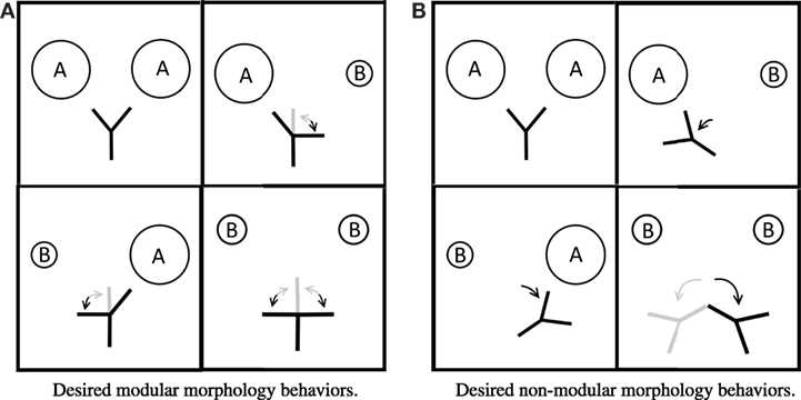
Figure 2. Drawings of desired behavior for the modular morphology (A) and non-modular morphology (B) in each of the four environments in the 2 × 2. Arrows indicate desired movement away from the base position (the base position is shown in the top left panels). Gray segments and arrows indicate other acceptable behaviors.

Three environment spaces were considered.

The first was the simplest consisting of a 2 × 2 environment space, giving four separate environments (Figure 3A). Each sphere could be Type A or Type B (n_p = 2). For this environment, the type A sphere had a radius of 3.5, and the type B sphere had a radius of 0.5.

FIGURE 3

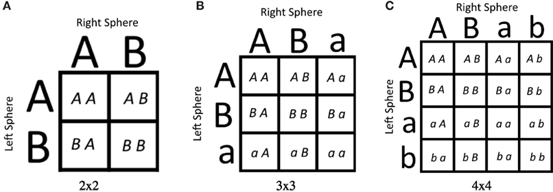
Figure 3. The three environment spaces considered. A, B, a, and b represent spheres positioned on the left or right of the robot. Uppercase letters represent bigger spheres than their lowercase counterparts. Robots were evolved to “point” at A = {A, a} spheres and away from B = {B, b} spheres. (A) represents the 2 × 2 environment space, (B) represents the 3 × 3 environment space, and (C) represents the 4 × 4 environment space.

The second environment space contained 3 × 3 environments, meaning nine total environments to consider (Figure 3B). A sphere could be one of two instances of Type A (either A or a) or Type B. For this environment, space A had a radius of 3.5, a had a radius of 0.5, and B was in the middle with a radius of 2.0. Thus, for this environment space, n_p = 3.

Finally, the last environment space considered contained 4 × 4 = 16 different environments (Figure 3C). A sphere could be one of two instances of Type A (A or a) or one of two instances of Type B (B or b). For this environment space, spheres of type A, B, a, and b had radii of 3.5, 2.5, 1.5, and 0.5, respectively. Therefore, n_p = 4 for this environment space.

Open Dynamics Engine was used to simulate the robots and the environment. A time step size of 0.05 was used.

2.4. Evolutionary Optimization

The robots were trained using Age-Fitness Pareto Optimization [AFPO; Schmidt and Lipson (2011)]. AFPO is a multi-objective optimization algorithm, which is designed to maintain diversity in an evolving population by periodically injecting new random individuals into the population and restricting the ability of older individuals to unfairly compete against younger individuals. In all of the experiments reported herein, a population size of 40 was employed.

Mutations in the population occurred in the form of choosing a new weight for a synapse from a normal distribution with mean of the current weight and a SD proportional to the absolute value of the current weight. This mutation operator enables evolution to rapidly incorporate high magnitude weights if required while also being able to fine tune weights with low magnitude. Mutation rates were set to be the reciprocal of the number of synapses, thus yielding an average of one synapse change per mutation.

The optimization function used was an error function, which averaged the error of the robot when exposed to each environment in the environment list E_{}:

$\begin{array}{l}\hfill \text{Err}\left(E_{\left\{\right\}}\right)=\frac{1}{||E_{\left\{\right\}}||}{\displaystyle \sum _{o_{\ell }{o}_r\in E_{\left\{\right\}}}}\frac{e\left(o_{\ell }{o}_r\right)-e_{\min }\left(o_{\ell }{o}_r\right)}{e_{\max }\left(o_{\ell }{o}_r\right)-e_{\min }\left(o_{\ell }{o}_r\right)}\end{array}$ (2)

$\begin{array}{l}\hfill e\left(o_{\ell }{o}_r\right)=\frac{g\left(o_{\ell }\right)+g\left(o_r\right)}{2}\end{array}$ (3)

$\begin{array}{l}\hfill \begin{array}{rl}g\left(A\right)& =\left\{\begin{array}{c}1,\text{if}d\left(A\right)>d_{\max }\left(A\right)\\ \frac{d\left(A\right)-d_{\min }\left(A\right)}{d_{\max }\left(A\right)-d_{\min }\left(A\right)},\text{otherwise},\end{array}\right.\\ g\left(B\right)& =\left\{\begin{array}{c}0,\text{if}d\left(B\right)>d_{\max }\left(B\right)\\ \frac{d\left(B\right)-d_{\min }\left(B\right)}{d_{\max }\left(B\right)-d_{\min }\left(B\right)},\text{otherwise}\end{array}\right.\end{array}\end{array}$ (4)

where

• E_{} is a single environment, e.g., (AA, bA, Bb, etc.);

• o_l ∈ {A,B} indicates the type of the object on the left. Either (o_l = A) or (o_l = B);

• o_r ∈ {A,B} indicates the type of the object on the right. Either (o_r = A) or (o_r = B);

• e(o_lo_r) indicates the robot’s error incurred in environment o_lo_r during the last time step;

• e_min(o_lo_r) and e_max(o_lo_r) indicate the minimum and maximum possible error the robot can incur in environment o_lo_r during any one-time step, respectively. These were calculated based on the environment present and the geometry of the robot;

• g(o_l) and g(o_r) denote the errors incurred as a result of the left-hand and right-hand objects, respectively;

• g(A) and g(B) denote the errors incurred as a result of the objects of each type.

• d(A) and d(B) denote the distances from the midpoint of the closest leaf to the center of the object considered.

• d_max(A), d_min(A), d_max(A), and d_min(B) denote the maximum and minimum distance values for the A and B environments. Because the motion range of the modular and non-modular robots is inherently different, these values are necessarily different. Further, the d_max(A) and d_max(B) values could be set artificially lower than the actual maximums in order to create weighting which more heavily considered g(A) term over g(B). d_min(A) and d_min(B) represent the actual observable minimums depending on the geometry of the robot. The values are presented in Table 1.

TABLE 1

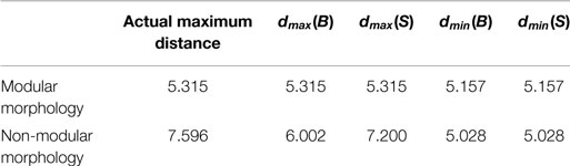
Table 1. Table of maximum and minimum distance values for each morphology type.

For the modular morphologies, d_max was set to the actual limit of motion of the branch. For the non-modular morphologies, d_max was set to less than the actual range of the motor to produce the desired behavior. By setting d_max less than the actual range, any robot that goes past a certain distance away from the A sphere would have an error of 1 for that object. Similarly, in the B sphere, if the robot moved far enough away to be past d_max, it was considered to have 0 error. This effectively created a weighting to the influences between the A and B spheres, which corresponded to the robot learning the desired behavior as seen in Figures 2 and 4.

FIGURE 4

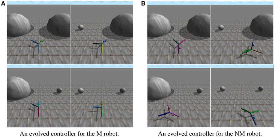
Figure 4. The behaviors generated by two controllers that evolved to succeed in each of the four environments in the 2 × 2 environment space. Lines emanating from the leaf branches represent the distance sensors embedded in each. Video of the robots can be found at https://www.youtube.com/watch?v=t4gjv5nYeAA. (A) depicts an evolved robot with a modular morphology in each of the four environments in the 2 × 2 environment space. (B) depicts an evolved robot with a non-modular morphology in each of the four environments in the 2 × 2 environment space.

2.5. Experimental Design

The first set of experiments consisted of evolutionary trials made up of fixed length epochs in the 2 × 2 environment space. The robot starts by training on one environment for the duration of the epoch. At the end of each epoch, a new environment is added for the robot to be trained on. By the last epoch, the robot is trained on all four environments. So, from the robots’ perspective, when each new environment was introduced, the environment space changes by becoming more complex. The epoch length was set to 100 generations; thus, each evolutionary run lasted for 400 generations. If a robot survived from the last generation of one epoch into the first generation of the next epoch, its fitness was recomputed against this expanded set of environments.

In the second set of experiments, the robots were evolved in a predetermined subset of the environment space. Unlike the previous experiment, the robot is introduced to all of the environments in the subset at the same time instead of sequentially. After the best robot in the population achieved a prespecified error threshold in all of the environments in the chosen subset, it was tested in the remaining environments, not in the subset, without any further evolution to see how well it performed.

3. Results

Experiment 1, described in Section 2.5, was run 50 times for all three robots in four environments in the 2 × 2 environment space, yielding a total of 50 × 2 = 100 independent evolutionary runs. The order of the environments was AA, BB, AB, and BA. Figure 5 shows that at the start of each epoch, there is a spike in the error in the case of both the MNM and NM robots. In the case of the M robot, there is no spike in error when the third (AB) and fourth (BA) epochs are introduced.

FIGURE 5

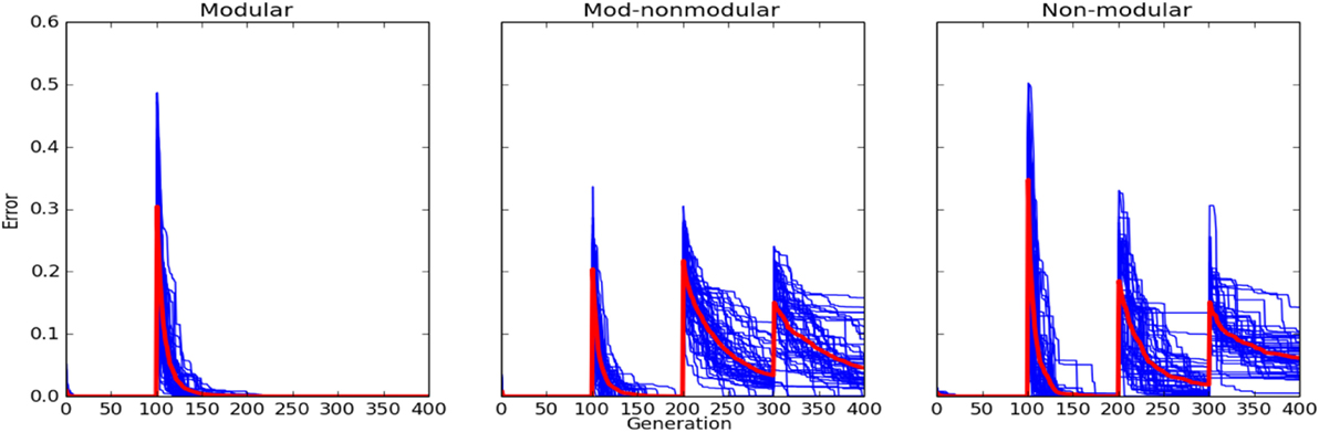
Figure 5. Errors of controllers evolved for the M robot (left column), MNM robot (middle column), and the NM robot (right column) in fixed epoch training (Experiment 1 as described in Section 2). New environment regimes occurred every 100 generations. Robots were evolved along the diagonal of the environment space meaning the order presented to the robot was AA, BB, AB, and BA. Each blue curve corresponds to an individual evolutionary run: it reports, at each generation, the controller with the lowest error in the population at that time. The red curve reports the average of these runs.

Experiment 2, described in section 2.5, was also run 50 times for the 2 × 2, 3 × 3, and 4 × 4 environments on all of the robots. Thus, there were 50 × 2 × 3 = 300 independent trials. For the first set of trials, only the “diagonal” of the environment space was considered. For the 2 × 2 environment space, this consisted of {AA, BB}. For the 3 × 3 environment space, the diagonal was {AA, BB, aa}. Finally, for the 4 × 4 environment space, the diagonal was {AA, BB, aa, bb}. The error threshold was set to 0.15. Figure 6 shows the results for these trials.

FIGURE 6

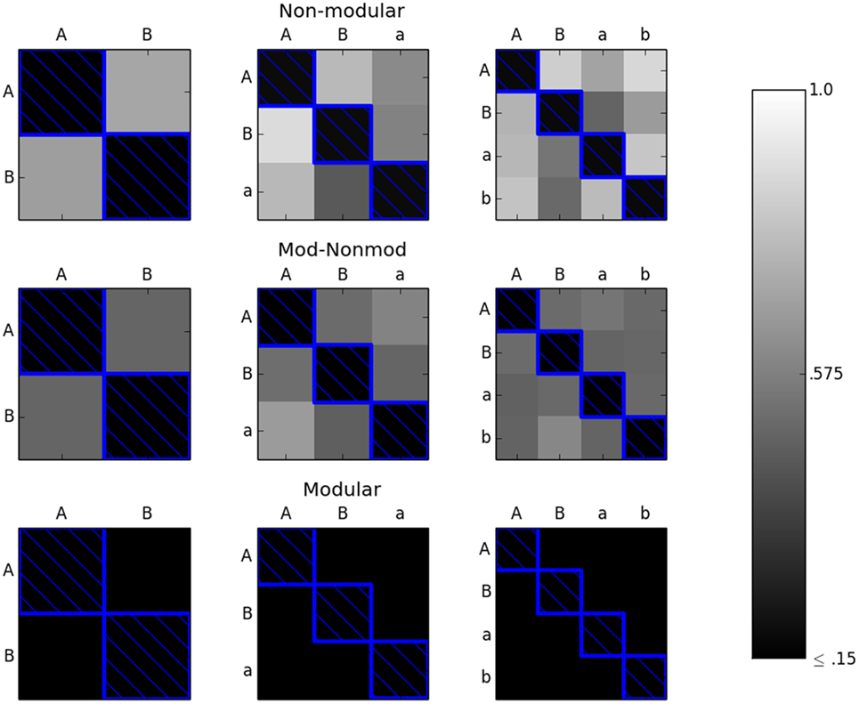
Figure 6. The M (bottom row), MNM (middle row), and NM (top row) robots were evolved along the diagonal (environments with blue boxes around them) until they achieved an error of less than or equal to 0.15 in each environment in the subset considered. The robots were then tested in the remaining environments. The color of the box of each environment represents the average reported error in that environment. The lighter the color, the greater the average error with white representing an error of 1.0 and black representing an error of ≤0.15. In the modular case, every robot achieved an error of less than or equal to 0.15 on the off-diagonal environments. Over the 50 trials, both the non-modular and mod-non-modular robots averaged an error greater than 0.15 in all of the off-diagonal environments.

The next test using this experimental setup considered another subset other than the diagonal, which had the same number of elements as the diagonal. Specifically, the “corner” of the environment space was considered Figure 7. All the three environment spaces were considered. For the 2 × 2 environment space, the corner was designated to be the top row of the environment space {AA, AB}. For the 3 × 3 environment space, the corner was set as {AA, AB, BA}. Finally, for the 4 × 4 environment space, the corner was {AA, AB, BA, BB}. Fifty trials of each robot in each environment space were performed, yielding 50 × 2 × 3 = 300 independent trials. Again, the error threshold was set to 0.15.

FIGURE 7

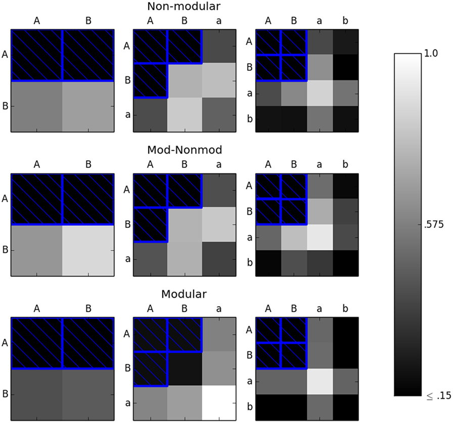
Figure 7. The M (bottom row), MNM (middle row), and NM (top row) robots were evolved in the corners (environments with blue boxes around them) until they achieved an error of less than or equal to 0.15 in each environment in the subset considered. The robots were then tested in the remaining environments. The color of the box of each environment represents the average reported error in that environment. Here, we see that it is necessary to use completely independent subsets of environment to ensure linear scaling in the modular case.

The last test performed using this experimental setup looked at how well the MNM and NM robots respond to an unseen environment in the 2 × 2 case when evolved in three out of the four environments. The robots were evolved in three different subsets: {AA, AB, BA}, {AA, AB, BB}, and {AB, BA, BB}. Because of the inherent symmetry in the problem, {AA, AB, BB} is the same as {AA, BA, BB}; so, only one was chosen to be tested. Results are presented in Table 2.

TABLE 2

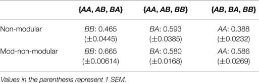
Table 2. Mean values of the error for the non-modular robot in the unseen environment after achieving an error of at most 0.15 in the three seen environments.

4. Discussion

When the modular robot is presented with a new environment, it is able to break down that environment into a combination of percepts. If the robot has seen those percepts before, even if the combination of those percepts is unfamiliar, it is able to act appropriately. Evidence for this is shown in Figure 5. There is no spike in error in the modular case at the start of the third and fourth epochs when the AB and BA environments are introduced. In contrast, the non-modular robots cannot see the environment in this manner, as is shown by the presence of error spikes at each new epoch.

Figure 6 shows that when the modular robot is evolved along the diagonal of the environment space, it is able to achieve acceptable error levels, that is at or below the predetermined cut off threshold (0.15), in the remaining environments in the environment space. This suggests that for this specific task, the number of environments needed to evolve a robot with a modular morphology and controller scales with the size of the diagonal of the environment space. Therefore, the necessary number of environments for the modular robot seems to scale linearly with n_p, where n_p is equal here to the number of variations in the size of the spheres.

Conversely, the robots with the non-modular morphologies or controllers do not achieve acceptable, at or below 0.15, errors in the other environments in the space by simply evolving along the diagonal, as seen in Figure 6. This means that for this task, the number of environments the robot needs to be evolved in before achieving adequate fitness for the whole environment space is greater than the number of environments along the diagonal.

Table 2 shows that even when either of the non-modular robots is presented with three out of the four environments in the 2 × 2 environment space, they cannot use what it has seen in previous environments to help them in the unseen environment. Thus, at least for the 2 × 2 environment space case, the non-modular robots need to be evolved in each environment in the entire space in order to achieve adequate fitness.

Figure 7 indicates that just choosing any subset of environments to evolve in does not guarantee adequate fitness in the remaining unseen environments. Specifically, the results point to choosing a subset of environments in which each environment is completely independent from every other environment in the subset. In this context, completely independent environments are those which do not share the same row or column. For example, AB would be completely independent from aa since both the right (A ≠ a) and left (B ≠ a) spheres are different. As a converse example, AB and Aa are not completely independent since the left sphere is the same in both environments, namely, A. These results further suggest that a modular robot can recognize familiar precepts from previous environments and respond appropriately to them, even when they are presented in an unfamiliar combination. This is seen in the result from Figure 7, which shows that in the 3 × 3 environment space case, when the robot is tested in the BB environment, it reacts appropriately without requiring further evolution.

Figure 7 also shows the side result that evolution will generally find the simplest action to solve the problem at hand. In the 4 × 4 environment space case, both the modular and non-modular robots evolve to act on any sphere of size B or smaller (the a or b sizes) as an instance of the B sphere. Thus, the robots do well in the remaining environments comprised of b spheres and poorly in the environments containing a spheres since the action desired for B sizes is the same as b and different than the action desired for a.

5. Conclusion

This paper has shown that a modular morphology, combined with a modular neural control, can enable a robot to break down seemingly novel environments into combinations of familiar percepts. Moreover, if robots possess both this morphological and neural modularity, these robots are also likely to move in a similar manner in these environments, thus continuing to perceive the environment as a combination of familiar percepts. Assuming that the robot should always react the same way to each of these local percepts, it follows then that such a robot is likely to exhibit a successful behavior in this novel environment without requiring further training.

Robots with either non-modular morphologies or non-modular neural controllers cannot easily exhibit this phenomenon and, as a result, are likely to require additional training even in environments that contain individually familiar percepts. Given this, we have shown that for this task, robots with a modular morphology, combined with a modular neural controller, need to be evolved only in a linearly growing number of environments, whereas the number of environments non-modular robots require grows superlinearly. Our results indicate that it is likely that non-modular robots will require evolution in all of the possible environments in the space.

In future work, we would like to investigate specifically how the amount of evolutionary time necessary to evolve adequately fit robots scales for both the modular and non-modular robots. We plan to accomplish by completely evolving both the modular and non-modular robots in the 2 × 2, 3 × 3, and 4 × 4 environment spaces. Further, we will look into scaling both f and n_p instead of just n_p, as was presented in this work.

If we consider our entire environment space to be a hypercube composed of $n_p^f$ hypervoxels representing each individual environment, then there will be n_p voxels along the diagonal of the hypercube. If it is sufficient for a modular robot to simply evolve along this diagonal, then it is possible for time complexity, in this case the number of evolutionary time steps, necessary to evolve a given robot in an $n_p^f$-sized environment space to decrease from $O\left(n_p^f\right)$ to O(n_p). However, this ideal case holds only if the robots are already morphologically and neurologically modular.

If robots begin with little or no morphological or neural modularity, it follows from Kashtan and Alon (2005) that if environments are added in a modularly varying way, more modular robots should evolve. This can be accomplished in this framework by ensuring that each newly added environment contains just one new feature of one of the free parameters describing the environments, while the other free parameters hold to a feature against which the robots have already been trained. This would require environments to be added to the training set along each of the edges of the environment hypercube in sequence, thus reducing $O\left(n_p^f\right)$ to O(n_pf). Determining whether this theoretical result holds in practice, and under what conditions, is another worthy target of future investigation.

There are many other problems to investigate, including how these results here can be generalized to more complex and realistic robots and task environments; furthermore, under what conditions would the evolved modularity be maintained when the evolved robots are instantiated as physical robots.

Ultimately, this work thus suggests that there may exist a relationship between morphology, modularity, evolvability, and scalability, which may in future enable the automated optimization of increasingly complex robots that perform appropriately in increasingly complex environments.

Author Contributions

CC – coding, data analysis, and experimental setup. JB – experimental design and inspiration; heavy review and editing. AB – heavy review and editing; contributions to simulations. KL – heavy review and editing; experimental design. NL – heavy review and editing; contributions to simulations.

Conflict of Interest Statement

The authors declare that the research was conducted in the absence of any commercial or financial relationships that could be construed as a potential conflict of interest.

Acknowledgments

This work was supported by National Science Foundation awards INSPIRE-1344227 and PECASE-0953837. The authors would also like to thank John Long, Jodi Schwarz, and Marc Smith of Vassar College for innumerable discussions that contributed indirectly to this work.

Code

Source code can be found at https://github.com/ccappelle/TreebotFrontiers

References

Bernatskiy, A., and Bongard, J. C. (2015). “Exploiting the relationship between structural modularity and sparsity for faster network evolution,” in Proceedings of the Companion Publication of the 2015 on Genetic and Evolutionary Computation Conference (Madrid: ACM), 1173–1176.

Google Scholar

Bongard, J. C. (2011). “Spontaneous evolution of structural modularity in robot neural network controllers,” in Proceedings of the 13th Annual Conference on Genetic and Evolutionary Computation (Dublin: ACM), 251–258.

Google Scholar

Bongard, J. C., Bernatskiy, A., Livingston, K., Livingston, N., Long, J., and Smith, M. (2015). “Evolving robot morphology facilitates the evolution of neural modularity and evolvability,” in Proceedings of the 2015 on Genetic and Evolutionary Computation Conference (Madrid: ACM), 129–136.

Google Scholar

Brooks, R. A. (1990). Elephants don’t play chess. Rob. Auton. Syst. 6, 3–15. doi: 10.1016/S0921-8890(05)80025-9

CrossRef Full Text | Google Scholar

Clark, A. (1998). Being There: Putting Brain, Body, and World Together Again. Cambridge: MIT press.

Google Scholar

Clune, J., Mouret, J.-B., and Lipson, H. (2013). The evolutionary origins of modularity. Proc. R Soc. B Biol. Sci. 280, 20122863. doi:10.1098/rspb.2012.2863

PubMed Abstract | CrossRef Full Text | Google Scholar

Ellefsen, K. O., Mouret, J.-B., and Clune, J. (2015). Neural modularity helps organisms evolve to learn new skills without forgetting old skills. PLoS Comput. Biol. 11:e1004128. doi:10.1371/journal.pcbi.1004128

PubMed Abstract | CrossRef Full Text | Google Scholar

Espinosa-Soto, C., and Wagner, A. (2010). Specialization can drive the evolution of modularity. PLoS Comput. Biol. 6:e1000719. doi:10.1371/journal.pcbi.1000719

PubMed Abstract | CrossRef Full Text | Google Scholar

Fitch, R., Stoy, K., Kernbach, S., Nagpal, R., and Shen, W.-M. (2014). Reconfigurable modular robotics. Rob. Auton. Syst. 7, 943–944. doi:10.1016/j.robot.2013.08.015

CrossRef Full Text | Google Scholar

French, R. M. (1999). Catastrophic forgetting in connectionist networks. Trends Cogn. Sci. 3, 128–135. doi:10.1016/S1364-6613(99)01294-2

PubMed Abstract | CrossRef Full Text | Google Scholar

Kashtan, N., and Alon, U. (2005). Spontaneous evolution of modularity and network motifs. Proc. Natl. Acad. Sci. U.S.A. 102, 13773–13778. doi:10.1073/pnas.0503610102

PubMed Abstract | CrossRef Full Text | Google Scholar

Kouvaris, K., Clune, J., Kounios, L., Brede, M., and Watson, R. A. (2015). How evolution learns to generalise: principles of under-fitting, over-fitting and induction in the evolution of developmental organisation. arXiv preprint arXiv:1508.06854.

Google Scholar

Lipson, H., Pollack, J. B., and Suh, N. P. (2002). On the origin of modular variation. Evolution 56, 1549–1556. doi:10.1554/0014-3820(2002)056[1549:OTOOMV]2.0.CO;2

PubMed Abstract | CrossRef Full Text | Google Scholar

Matarić, M., and Cliff, D. (1996). Challenges in evolving controllers for physical robots. Rob. Auton. Syst. 19, 67–83. doi:10.1016/S0921-8890(96)00034-6

CrossRef Full Text | Google Scholar

Newman, M. E. (2006). Modularity and community structure in networks. Proc. Natl. Acad. Sci. U.S.A. 103, 8577–8582. doi:10.1073/pnas.0601602103

PubMed Abstract | CrossRef Full Text | Google Scholar

Pfeifer, R., and Bongard, J. (2006). How the Body Shapes the Way We Think: A New View of Intelligence. MIT press.

Google Scholar

Pinville, T., Koos, S., Mouret, J.-B., and Doncieux, S. (2011). “How to promote generalisation in evolutionary robotics: the progab approach,” in Proceedings of the 13th Annual Conference on Genetic and Evolutionary Computation (Dublin: ACM), 259–266.

Google Scholar

Schmidt, M., and Lipson, H. (2011). “Age-fitness pareto optimization,” in Genetic Programming Theory and Practice VIII, eds R. Riolo, T. McConaghy, and E. Vladislavleva (New York: Springer), 129–146.

Google Scholar

Wagner, G. P. (1996). Homologues, natural kinds and the evolution of modularity. Am. Zool. 36, 36–43. doi:10.1093/icb/36.1.36

CrossRef Full Text | Google Scholar

Yim, M., Shen, W.-M., Salemi, B., Rus, D., Moll, M., Lipson, H., et al. (2007). Modular self-reconfigurable robot systems [grand challenges of robotics]. Rob. Autom. Mag. IEEE 14, 43–52. doi:10.1109/MRA.2007.339623

CrossRef Full Text | Google Scholar