Morphological Computation Increases From Lower- to Higher-Level of Biological Motor Control Hierarchy

1. Introduction

In biological systems, voluntary movements are generated through a sequence of different processing units. From the motor cortex to the spinal cord to the stimulation signal running down the motor neuron to the muscle membrane. These processing units can be interpreted as a neurological, hierarchical control system (Loeb et al., 1999; Karniel, 2011). While it seems obvious that the neuronal structures are responsible for the initiation and execution of goal-directed movements, it has been discussed that also the morphology of a system contributes to the control (Iida and Pfeifer, 2004; Pfeifer and Iida, 2005; Paul, 2006; Blickhan et al., 2007; Ghazi-Zahedi et al., 2016). In particular in human arm movements, several control theories explicitly rely on the viscoelastic muscle characteristics to generate dynamic movements [e.g., impedance control Hogan, 1984, equilibrium point control Kistemaker et al., 2006, 2007a,b; Bayer et al., 2017]. Here, the muscles serve as a low-level zero-delay reflexes [termed preflexes Brown et al., 1995] capable of stabilizing the system against external perturbations (van Soest and Bobbert, 1993; Gerritsen et al., 1998; Loeb et al., 1999; Haeufle et al., 2010; Proctor and Holmes, 2010; John et al., 2013). Such contributions of the morphology have been termed “intelligence by mechanics” (Blickhan et al., 2007), “exploitive actuation” (Rieffel et al., 2010; Haeufle et al., 2012; Kalveram et al., 2012), or “morphological computation” (Pfeifer and Iida, 2005; Paul, 2006; Ghazi-Zahedi et al., 2016). Morphological computation, in this sense, captures the concept that control is partially performed by the controlled system interacting with the environment. More precisely, that part of the information processing necessary to generate a desired movement is performed by the morphological characteristics of the system, i.e., by its hard- or wet-ware.

Characterizing this contribution of the system's morphology to its behavior is possible by quantifying morphological computation (MC) (Zahedi and Ay, 2013; Ghazi-Zahedi et al., 2016; Ghazi-Zahedi, 2019). This requires a causal model of a reactive system's sensorimotor loop. The model must allow a clear separation of the system into a controller, actuator signals, sensor signals, and the physical system termed world, which includes the environment (in engineering this is typically called the plant). In a nutshell, the quantitative measure of morphological computation (MC_W) then quantifies the contribution of the world state W and the actuator signal A to the further time evolution of the world state, i.e., the next world state W′. MC_W is high, if the current world state W has a strong influence on the next world state W′, i.e., the system exploits its physical properties. Thus, it is possible to quantify morphological computation in causal models where A and W can be observed, e.g., in neuro-muscular models (Ghazi-Zahedi et al., 2016).

The open question is, however, where in the biological control system A and W should be separated. Is A the output of the neurons that innervate the muscles (α motor neurons) and therefore initiate muscle contraction? Or is A much higher in the control hierarchy: the output of the central nervous system, i.e., the signals that initiate a movement? One could argue for the latter separation, as the decentralized low-level control circuits, like mono-synaptic reflexes, are hard-wired into the spinal cord and are therefore rather part of the system than part of the controller. Or has A even to be located much lower in the control hierarchy: the output force of the muscles? The argument for this level of separation would be that muscles with their non-linear viscoelastic properties serve as low-level zero-delay reflexes (preflexes) contributing to control. Furthermore, they adapt during our life-time to the requirements of our daily activities. From our point of view it is unclear where to separate between W and A and how this decision influences the calculation of MC. Furthermore, it is unclear, to which extend higher-level control can exploit morphological computation of the lower-level structures—in actual units of bit.

This is not only relevant for the understanding of biological systems, but also for bio-inspired and bio-mimetic robotics. Much effort has been taken to develop new robotic design concepts exploiting material properties (Kim et al., 2013; Rus and Tolley, 2015; Polygerinos et al., 2017), such as viscoelastic muscle-like actuators in arm movements (Boblan et al., 2004; Driess et al., 2018), elasticity in legged locomotion (Iida et al., 2009; Niiyama et al., 2012; Hutter et al., 2013; Sprowitz et al., 2013; Hubicki et al., 2016; Ruppert and Badri-Spröwitz, 2019) or morphology which empowers hopping (Nurzaman et al., 2015), goal-directed swimming (Manfredi et al., 2013), crawling Shepherd et al. (2011), or even grasping (Deimel and Brock, 2016). However, also in these approaches, the hierarchy of morphological computation has not yet been quantified.

The purpose of this study was therefore to investigate morphological computation in a hierarchical control system. The novelty of our approach was to quantify morphological computation on different control levels to better understand the hierarchy. This is relevant for two reasons: (1) it further evaluates and validates the quantification concept of MC and (2) shows how the biological control system may benefit from its hierarchical control structure and its non-linear actuators, i.e., the muscles. For this, we resort to computer simulations of human arm movements with a model that considers joint dynamics, muscles, reflexes, central pattern generators, and higher-level control.

2. Methods

To investigate morphological computation in a hierarchical control system, we simulate human arm movement with a neuro-musculoskeletal model (Stollenmaier et al., 2020a) (see also Supplementary Material). In this model, it is possible to access all state signals, i.e., the state of the control logic, the input to the low-level controller, the control signal, the muscles' active state (biochemistry), the muscles' force, the generated joint torques, and the resulting joint angles (section 2.1). Thus, we can access all levels of the neuro-muscular control hierarchy to quantify morphological computation (section 2.3).

2.1. Neuro-Muscular Model

The neuro-muscular model of human arm movements has been developed to study neuronal motor control concepts in the interaction with the musculoskeletal model. For this purpose, we combined a computational motor control model of goal-directed arm movements with a musculoskeletal model (Figure 2). We will shortly summarize the approach here and refer to the Supplementary Material for the details of the model.

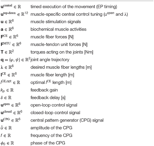
The model consists of several hierarchical layers (Figure 1), which we will describe shortly in the following, starting from the lowest hierarchical level (right-hand side). The chosen model parameters represent a generic man and are collected from different sources (van Soest and Bobbert, 1993; Kistemaker et al., 2006; Mörl et al., 2012; Bhanpuri et al., 2014 and others, listed in detail in the Supplementary Material).

FIGURE 1

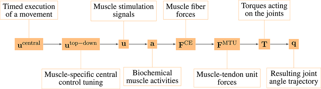
Figure 1. Overview over the hierarchy levels in our neuro-muscular model of the arm.

FIGURE 2

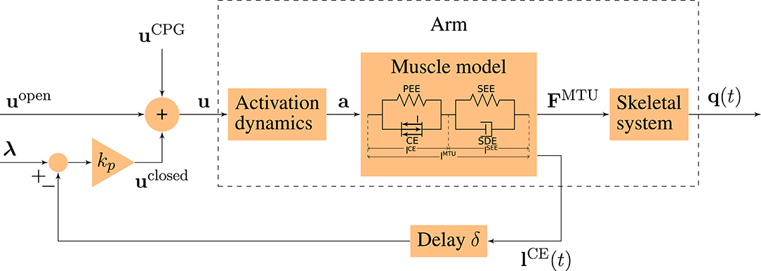
Figure 2. Schematic diagram of the motor control model. The motor command u is a sum of an open-loop and a closed-loop signal. The time-delayed feedback loop incorporates proprioceptive feedback (mono-synaptic reflexes) by comparing the actual muscle fiber lengths l^CE(t) to desired values λ. q(t) = (φ(t), ψ(t)) contains the elbow and shoulder angle, respectively.

2.1.1. Angles

The musculoskeletal model predicts two-degree-of-freedom arm movements in the sagittal plane (see Figure 3). Its dynamics are determined by two rigid bodies (lower and upper arm) that are connected via two one-degree-of-freedom revolute joints that represent the shoulder and elbow joint. This can be described by double-pendulum equations of motion, i.e., second-order ordinary differential equations. The outputs of this layer are the predicted joint angles which correspond to the experimentally observable state (q ∈ ℝ²).

FIGURE 3

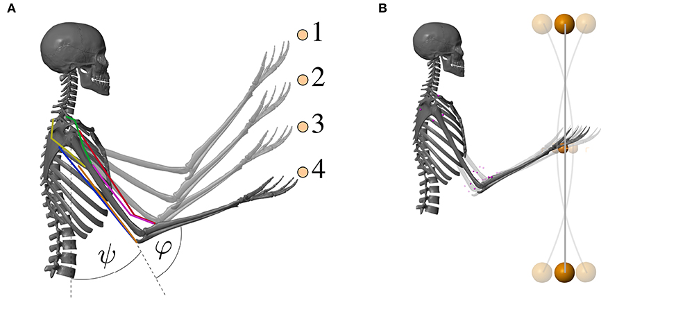
Figure 3. Visualization of the musculoskeletal model that was used for the computer simulations of the arm movements. The colored lines represent the modeled muscles. (A) Goal-directed point-to-point movement between the points 1–4 and (B) dynamic oscillation movements with a vibrating rod.

2.1.2. Torques

The rigid bodies are driven by joint torques, which are calculated based on anatomical muscle paths (Hammer et al., 2019) and translating forces at the muscle origin, insertion, and via-points into joint torques. The outputs of this layer are the predicted joint torques (T ∈ ℝ²).

2.1.3. Muscle-Tendon Unit Forces

Active forces are generated by six muscle-tendon units (MTUs), four monoarticular and two biarticular muscles. The force of each MTU is modeled using a Hill-type model accounting for muscle fiber and tendon characteristics (Haeufle et al., 2014). The dynamic of each MTU is modeled by a first-order ordinary differential equation. The outputs of this layer are the predicted muscle-tendon unit forces (F^MTU ∈ ℝ⁶).

2.1.4. Muscle Fiber Forces

The model of the muscle fibers, termed contractile elements (CE), considers the dependence of the active fiber force on fiber length and contraction velocity known from biological muscle fibers. The outputs of this layer are the predicted muscle fiber forces (F^CE ∈ ℝ⁶).

2.1.5. Biochemical Muscle Activity

The biochemical processes that lead from a neuronal muscle stimulation to a force generation can be modeled by a first-order ordinary differential equation. The implemented model of the activation dynamics further considers the fiber length dependency of this process (Hatze, 1977; Rockenfeller et al., 2015). The outputs of this layer are the predicted muscle fiber activity states (a ∈ ℝ⁶).

2.1.6. Muscle Stimulation Signals

The bio-inspired hybrid equilibrium point controller exploits muscle characteristics by combining a feed-forward command [u^open(t)] with spinal feedback on muscle fiber lengths [u^closed(t)]. This feedback represents a simplified version of the mono-synaptic muscle spindle reflex, assuming that the muscle spindles provide accurate time-delayed information about the muscle fiber lengths l^CE(t) (Kistemaker et al., 2006). The total motor command u_i for each muscle i is a sum of those components and is calculated as

$\begin{array}{ll}\begin{array}{l}{u}_i(t)={\left\{u_i^{\text{open}}(t)+u_i^{\text{closed}}(t)+u_i^{\text{CPG}}(t)\right\}}_0^1\\ ={\left\{u_i^{\text{open}}(t)+\frac{k_p}{l^{\text{CE,opt}}}\left({\lambda }_i(t)-l_i^{\text{CE}}(t-\delta )\right)+u_i^{\text{CPG}}(t)\right\}}_0^1,\end{array}& (1)\end{array}$

where k_p is a feedback gain and the time delay δ is set to 10 ms representing a short-latency reflex delay which is in a physiologically plausible range (More et al., 2010; Houk and Rymer, 2011). l^CE,opt stands for the optimal length of the contractile element. The operation ${\{x\}}_0^1$ sets values x < 0 to 0 and x > 1 to 1. The signal $u_i^{\text{CPG}}$ represents a central pattern generator (CPG). The outputs of this layer are the predicted muscle stimulation signals (α motor neuron activities u ∈ ℝ⁶).

2.1.7. Muscle-Specific Central Control Tuning

The low-level controller gets two top-down input signals: The open-loop muscle stimulation $u_i^{\text{open}}(t)$ and the desired muscle fiber lengths λ_i(t). Here, they represent an intermittent control approach, because they are piecewise constant functions over time. Herein, each constant value represents an equilibrium posture (EP), i.e., the system is in a stable equilibrium in these positions. The calculation of these central control signals for a given movement is described in detail in the Supplementary Material. The outputs of this layer are the top-down central commands to each low-level reflex circuit (u^top-down ∈ ℝ¹²).

2.1.8. Timed Execution of a Movement

The output of our highest level of motor control is a single piecewise constant signal used to time the selection of equilibrium points meaning that all sub-circuits are switched at the same time (u^central ∈ ℝ¹).

2.2. Simulation Experiments

2.2.1. Movement 1: Point-to-Point Movements

The first movement investigated here is a point-to-point movement along a vertical line. Different movements between four target positions were evaluated (see Figure 3A and Supplementary Material). The central pattern generator is inactive for those movements [u^CPG(t) = 0]. An animation of the movement is provided as Supplementary Material.

To consider the natural variation of this movement, we repeated the simulation of the movement 1 → 4 seven times. Each simulation only differed in the equilibrium postures (EPs) for the starting joint angles, the peak elbow joint angle, and the target joint angles. We determined these angles from motion capture data of a single subject performing the movement seven times. This natural variation of the angles resulted in different signals on the muscle-specific central control level, i.e., different u^top-down signals. All other parameters of the controller were kept constant.

2.2.2. Movement 2: Dynamic Oscillatory Movements

For the second movement, a vibrating rod was added to the hand in the model (see Figure 3B). The technical specifications of the rod can be found in the Supplementary Material. To excite the rod, as done in training and rehabilitation exercises, a sinusoidal signal u^CPG mimicking the output of a central pattern generator (CPG) is added to the motor command u:

$\begin{array}{ll}{\text{u}}^{\text{CPG}}(t)=\widehat{u}·sin(2\pi ·f^{\text{CPG}}·t+{\varphi }_0),& (2)\end{array}$

with û = 0.1: amplitude, f^CPG: frequency, ϕ₀: phase. The muscles are synchronized by setting ϕ₀ = 0 for flexing muscles and ϕ₀ = π for extending muscles.

The oscillation is exited for 0 ≤ t ≤ 4s. After this, u^CPG = 0 and the oscillation is then only a result of the dynamics of the system and not of the controller anymore. An animation of the movement is provided as Supplementary Material.

To consider the natural variation of this movement, we analyzed the frequency pattern of a single subject performing a swing-rod exercise. The fast-fourier-transform spectrum indicates a frequency variance of 0.2Hz. We therefore repeated the simulation 14 times with a set of random CPG frequencies f^CPG = 3.8 ± 0.2Hz.

2.2.3. Details on the Human Experiments to Estimate Natural Variability

Two healthy subjects participated in the study. The experimental procedure was approved by the local ethics committee (886/2018BO2). All participants gave their informed consent prior to participation. The movements were recorded with a 12-camera motion capturing system (Vicon Motion Systems Ltd, UK) using a marker set with 29 retro-reflecting markers. Using the recorded marker positions over time, shoulder and elbow angles were reconstructed (Rettig et al., 2009). The reconstructed joint angle trajectories were smoothed with a Savitzky-Golay polynomial filter (of order 4 and with a window size of 41 sampling points).

2.3. Quantifying Morphological Computation

The following paragraphs will only give a brief introduction to the quantification of MC. For a full discussion on this issue, please read (Ghazi-Zahedi, 2019) or the Supplementary Material to this publication. Quantifying MC requires a causal model of the sensorimotor loop which divides a cognitive system into a brain, actuators, environment, and sensors. In the context of this work, we are focusing on reactive systems which means that the actuators are directly connected with the sensors. A cognitive system is then fully described by the following set of Markov processes:

$\begin{array}{ll}\beta :{W}\to {\Delta }_{{S}}\left[\beta \left(s|w\right)\right]& (3)\end{array}$

$\begin{array}{ll}\pi :{S}\to {\Delta }_{{A}}\left[\pi \left(a|s\right)\right]& (4)\end{array}$

$\begin{array}{ll}\alpha :{W}\times {A}\to {\Delta }_{{W}}\left[\alpha \left(w^{\prime }|w,a\right)\right],& (5)\end{array}$

where $w\in {W}$ is the value of the world state W, $s\in {S}$ is the value of the sensor state S, and $a\in {A}$ is value of the actuator state A. We call β(s|w) the sensor map, as it describes how the agents perceive the environment, π(a|s) the policy, as it describes how the agent chooses an action as a reaction to a sensor, and finally we call α(w′|w, a) the world dynamics kernel, as it describes how the next world state W′ depends on the current world state W and the current action A. It is important to note here that the world state W captures everything physical. This means that the world state W captures the state of the system's body and its environment.

To quantify MC, we take a closer look at the world dynamics kernel α(w′|w, a). Assume that the next world state W′ does not depend on the current world state W but only on the current action A. This means that the world dynamics kernel reduces to $\tilde{\alpha }(w^{\prime }|a)$. In this case, it is fair to say that the system shows no MC at all, since the behavior is fully controlled by the action A. Any measured divergence from this assumption means that the current world state W had an influence on the next world state W′, and hence, the system is exploiting the physical properties of its body and its interactions with the environment. This can be measured by the Kullback-Leibler Divergence (Cover and Thomas, 2006) in the following way:

$\begin{array}{ll}{\text{MC}}_{\text{W}}:={\displaystyle \sum _{w^{\prime },w,a}}p(w^{\prime },w,a){log}_2\frac{\alpha \left(w^{\prime }|w,a\right)}{\tilde{\alpha }\left(w^{\prime }|a\right)}.& (6)\end{array}$

The output of our models contains discrete numerical data, i.e., S, A, and W are discrete variables. Therefore, we will summarize the approach for discrete variables here. For a discussion on how to estimate MC_W on continuous state spaces, please see Ghazi-Zahedi (2019).

The joint distribution p(w′, w, a) can be estimated by a frequency method, i.e., by counting the number of occurrences of each triplet (w′, w, a) normalized by the number of samples in the data. This leads to the following estimation for p(w′, w, a):

$\begin{array}{ll}p(w^{\prime },w,a)=\frac{c_{w^{\prime },w,a}}{N},& (7)\end{array}$

where $c_{w^{\prime },w,a}$ is the number of occurrences of (w′, w, a) and N is the total number of samples.

MC_W can now be calculated in the following way:

The value calculated in line 9, MC_W, represents the morphological computation primarily used in this work. Sometimes it is further interesting to take a look at the state-dependent morphological computation, i.e., the time evolution of the quantity. This requires minimal changes to the original algorithms. Instead of calculating the probability-weighted sum over all states (line 9 in Algorithm 1), which leads to a single number as a result, the measures are evaluated n-tuple in the data set. This means that for MC_W, the logarithm is evaluated for every triple w_t+1, w_t, a_t (see Algorithm 2).

ALGORITHM 1

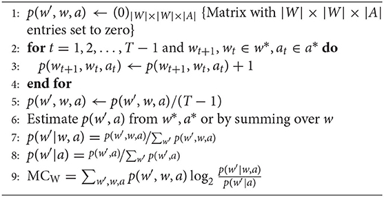
Algorithm 1. Algorithm for MC_W.

ALGORITHM 2

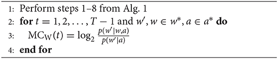
Algorithm 2. Algorithm for state-dependent MC_W(t).

In conclusion, in order to quantify MC, we need time signals of the World and Actuator states, W and A, respectively. This means that it is necessary to separate the state variables of the system into W and A.

The neuro-muscular model investigated here has several hierarchical levels (Figure 1). For this study, we systematically separated the state variables between all of these different hierarchy levels and calculated MC for each possible hierarchy level.

There are two possible approaches to select W and A and then calculate MC (Figure 4): The first approach (Figure 4A) relates to the evaluation of experimental data, where usually not all state variables can be recorded (especially in biological systems). Here, W is always the mechanical system state q(t), i.e., the joint positions (and for the oscillation movement also the position of the rod mass relative to the hand). A on the other hand contains only signals of one hierarchy level. We term this approach “selected hierarchy levels” and term the respective morphological computation ${\text{MC}}_{\text{W}}^{\text{sel}}$.

FIGURE 4

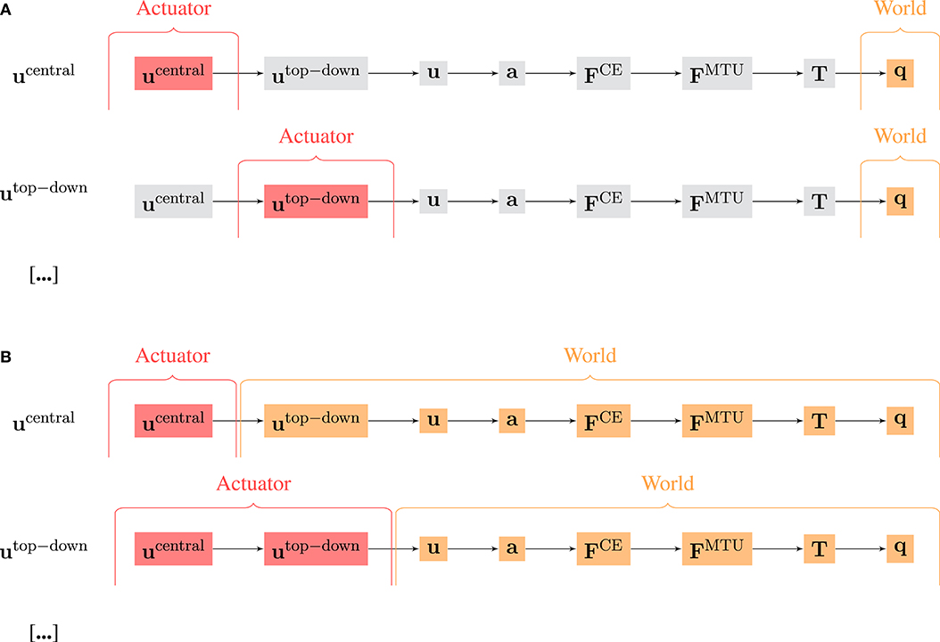
Figure 4. Visualization of the difference of the calculation of MC_W using (A) selected and (B) accumulated hierarchy levels as actuator signal A and world state W. Note that for the oscillation movements, the observable state q includes both the joint angles and the rod position.

The second approach (Figure 4B) always includes all signals. It represents a clear cut at a specific level. All signals below this cut-level are combined into W and all above into A. We termed this approach “accumulated hierarchy levels” and termed the respective morphological computation ${\text{MC}}_{\text{W}}^{\text{acc}}$.

2.4. Statistical Analysis

Each simulation run provides data to calculate morphological computation on all different hierarchy levels. Each hierarchy level is then quantified by a single scalar quantity MC_W representing the respective morphological computation (see line 9 in Algorithm 1). By varying the control parameters as described above, the resulting MC_W values represent a natural variation for the same movement. The hypothesis (H₀) was that there is no significant difference in MC between hierarchy levels across all repetitions of the movement. Each hierarchy thus represents a different group and we used ANOVA to test whether these groups differ. The normal distribution was tested with a Shapiro-Wilk test (with α = 0.1 to keep the beta error in check). The test confirmed normal distribution in the majority of the groups (17 out of 28). This should not influence the result, since ANOVA is robust to deviations form normal distribution, especially here where each group has the same number of samples. As the different hierarchy levels are taken from the same simulation, they are not independent. To test their statistical difference, we therefore analyzed the data with a repeated measures ANOVA. We further used a pairwise post-hoc test with Bonferroni correction to analyze which levels actually differ.

3. Results

Morphological computation is highest for the most central level of the control hierarchy investigated here (u^central). This holds for all four types of point-to-point movements we evaluated (Figure 5) as well as for the dynamic oscillation movement (Figure 7). Going further down in the control hierarchy, MC always decreases for the accumulated scenario (${\text{MC}}_{\text{W}}^{\text{acc}}$), and almost always for the selected (${\text{MC}}_{\text{W}}^{\text{sel}}$) with one exception: the torque. Choosing the torque T as actuator signal, the value for MC is higher than using one of the next higher-level signals of actuation. Please note that the figures are shown in logarithmic scale to allow a better comparison of the large differences between MC for the different hierarchy levels.

FIGURE 5

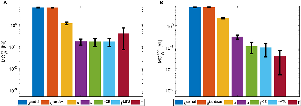
Figure 5. Point-to-point movement: Morphological computation MC_W on different hierarchy levels for an exemplary point-to-point movement (1 → 4, see Figure 3A). Morphological computation was evaluated using (A) selected (${\text{MC}}_{\text{W}}^{\text{sel}}$) and (B) accumulated hierarchy levels (${\text{MC}}_{\text{W}}^{\text{acc}}$). Note that a logarithmic scale is used for the y-axis. Shown are the mean ±1.96 times standard deviation (≈95% confidence interval) of seven simulation runs with different starting, intermittent, and target equilibrium postures taken from the natural variation observed in a human experiment. As tested by an ANOVA, there are significant differences in MC_W between the different hierarchy levels. The pairwise post-hoc test revealed that for ${\text{MC}}_{\text{W}}^{\text{sel}}$ there are two groups with similar mean: the highest two levels u^central, u^top-down, and the three levels a, F^CE, and F^MTU. The levels u and T differ from all others. For ${\text{MC}}_{\text{W}}^{\text{acc}}$, the three lowest levels F^CE, F^MTU, and T are one group. All other levels differ from all others. All significance levels were set to p < 0.05. The limit of the y-axis is set to the maximum MC value that would result from having a constant signal as input. Plots of the results of the other movements can be found in the Supplementary Material, but show the same trends.

In general, using accumulated hierarchy levels results in smaller morphological computation than using selected hierarchy levels (${\text{MC}}_{\text{W}}^{\text{acc}}<{\text{MC}}_{\text{W}}^{\text{sel}}$). Furthermore, pointing movements have a lower morphological computation than the dynamic oscillation movements.

The reproduction of the experimentally observed variation of the movement 1 → 4 in simulation also leads to a variation of MC_W. This variation is relatively small compared to the overall difference between hierarchy levels. Therefore, an ANOVA test reveals statistical significant differences between the hierarchy levels. However, not all levels are significantly different. Especially u^central and u^top-down, as well as F^CE and F^MTU do not differ significantly in MC.

3.1. Noise in Point-to-Point Movements

In the pointing movements, all state variables are smooth, which is a result of the noise-free formulation of the continuous control signals. Therefore, the highest control levels produce very simple control signals, i.e., piecewise constant signals in time (see above and Supplementary Material for more details).

To test whether this smooth definition has an influence on the result, we added random (uniformly distributed) noise to the muscle stimulation signals u [noise levels: medium: 40/300 · (u_max − u_min), high: 80/300 · (u_max − u_min)]. This changes the previously consistent trend: the higher the added noise, the lower the MC at the level of the muscle stimulation u (Figure 6). At the same time, MC between at the muscle activity level a increases. This leads to the fact, that—after adding noise to the stimulation signal - MC with u as actuator signal is lower than the calculation with a as actuator signal. However, this change in trend is only true if morphological computation is evaluated on selected signals (${\text{MC}}_{\text{W}}^{\text{sel}}$). For ${\text{MC}}_{\text{W}}^{\text{acc}}$, the trend is never reversed. Noise only slightly shifts the values (not shown).

FIGURE 6

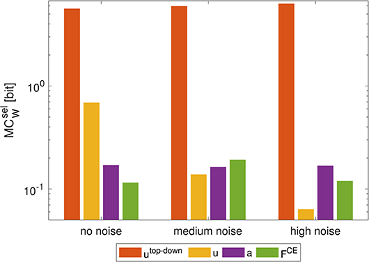
Figure 6. Influence of noise on morphological computation. Morphological computation for selected hierarchy levels (${\text{MC}}_{\text{W}}^{\text{sel}}$) for a point-to-point movement (1 → 4). The noise was added to the muscle stimulation u [noise levels: medium: 40/300 · (u_max − u_min), high: 80/300 · (u_max − u_min)]. As a result, ${\text{MC}}_{\text{W}}^{\text{sel}}$ at the muscle stimulation level decreases and increases in adjacent hierarchy levels. Note that a logarithmic scale is used for the y-axis.

3.2. Dynamic Oscillatory Movements

The general trend of decreasing morphological computation for lower hierarchy levels was the same in the dynamic oscillation movements (Figure 7).

FIGURE 7

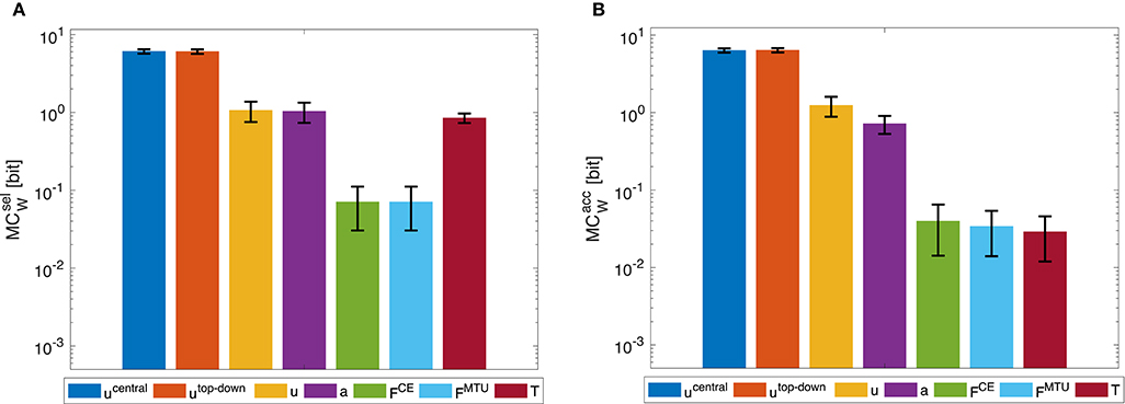
Figure 7. Dynamic oscillation movement: Morphological computation MC_W for (A) selected (${\text{MC}}_{\text{W}}^{\text{sel}}$) and (B) accumulated hierarchy levels (${\text{MC}}_{\text{W}}^{\text{acc}}$). Shown are the mean ±1.96 times standard deviation (≈95% confidence interval) of 14 simulation runs with a set of random CPG frequencies in the spectrum observed in a human experiment. As tested by an ANOVA, there are significant differences in MC_W between the different hierarchy levels. The pairwise post-hoc test revealed that for ${\text{MC}}_{\text{W}}^{\text{sel}}$, the highest levels u^central and u^top-down have similar means, so do the muscle stimulation u, activity a, as well as the forces F^CE and F^MTU. Only the torque level T differs from all other groups. For ${\text{MC}}_{\text{W}}^{\text{acc}}$, the highest levels u^central and u^top-down have similar means, so do the lowest levels F^CE, F^MTU, and T. All significance levels were set to p < 0.05. The limit of the y-axis is set to the maximum MC value that would result from having a constant signal as input. Note that a logarithmic scale is used for the y-axis.

However, the dynamic oscillation data has different phases. In the initial phase (t ≤ 4s), the rod is excited by sinusoidal muscle stimulation signals with a frequency tuned to the rod's resonance (Figure 9). In this phase, everything oscillates in sync and the morphological computation is on average smaller. Once the CPG is turned off (t > 4s), the control signals become relatively steady—only influenced by the feedback signals trying to hold the position. The rod, however, still has a lot of energy and therefore keeps oscillating. In this phase, MC_W increases. These results are similar on all levels of the control hierarchy (Figure 8). Interestingly, ${\text{MC}}_{\text{W}}^{\text{acc}}$ actually becomes zero on the lower hierarchy levels in the resonance oscillating movements between 2 ≤ t ≤ 4s. This means that muscle fiber force F^CE, muscle-tendon unit force F^MTU, and joint torques T contain the same information as the mechanical state of the system q.

FIGURE 8

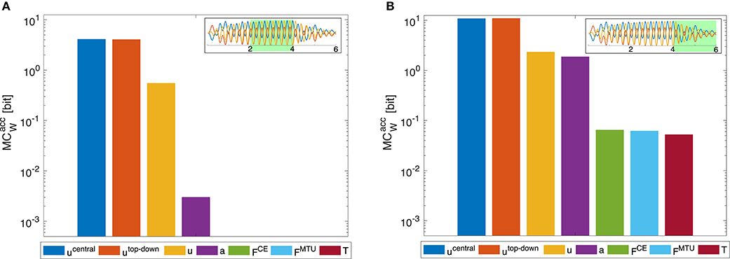
Figure 8. Dynamic oscillation movement. Morphological computation is higher for the last movement phase where the central pattern stimulation is deactivated and the movement continues due to the passive dynamics of the arm-rod system. (A) ${\text{MC}}_{\text{W}}^{\text{acc}}$ evaluated for the time span between 2 and 4 s (B) for the time span between 4 and 6 s, as indicated by the insets, which show the oscillation of the joints and the rod (cf. Figure 9). In the first time span, the control signals are sinusoidal muscle stimulations exciting the rod at its resonance frequency (f^CPG = 3.8Hz). In the second time span (B), the sinusoidal stimulation is zero and the oscillation is only driven by the dynamics of the rod. The limit of the y-axis is set to the maximum MC value that would result from having a constant signal as input. Note that a logarithmic scale is used for the y-axis.

4. Discussion

The meaning of morphological computation can be seen quite well in the example of the dynamic oscillations. In the initial phase, the controller enforces a dynamic oscillation at the system's resonance. In resonance, the morphological computation is then quite low, as most—or even all—information on the system state is already contained in the stimulation, activity, and muscle force signals (Figures 8A, 9). This is similar to a robotic model, driven by complex control signals (Ghazi-Zahedi et al., 2016). However, if the sinusoidal excitation is switched off, the rod dynamics take over and generate a rich dynamic behavior at almost no information input on the control/actuation levels. Hence, morphological computation is high (Figure 8B). This case is similar to, e.g., mechanical toys, such as passive dynamic walkers which generate the entire behavior based on their mechanical properties. This example confirms that the measure of MC_W captures what we would expect as morphological computation.

FIGURE 9

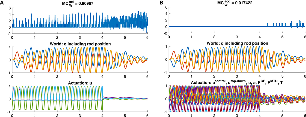
Figure 9. Time evolution of morphological computation MC_W, world state W and actuator state A for the dynamic oscillation movement. The oscillation is exited for 0 ≤ t ≤ 4s by a sinusoidal CPG stimulation signal. After this, u^CPG = 0 and the oscillation is then only a result of the dynamics of the system and not of the controller anymore. Shown here is exemplary (A) the case of ${\text{MC}}_{\text{W}}^{\text{sel}}$ of the muscle stimulation level u (yellow bar in Figure 7A) and (B) the case of ${\text{MC}}_{\text{W}}^{\text{acc}}$ including only the joint angles and rod position as world state (dark red bar in Figure 7B).

By measuring morphological computation in a hierarchical control system, we can—for the first time—quantify the contribution of different hierarchy-levels to the control. The increase of morphological computation for higher-levels of the control hierarchy in the accumulative evaluation (${\text{MC}}_{\text{W}}^{\text{acc}}$) means that the lower control levels actually contribute quite significantly. To be able to test whether the differences between the hierarchy-levels are significant, we introduced variations based on experimental data. Not all MC data generated in this way fulfills the ANOVA assumption of equal distribution for each group represented by a hierarchy level. Still, the results found by the ANOVA and post-hoc test match what can be seen in Figures 5, 7. Literature suggests this contribution of muscles to dynamic movements (van Soest and Bobbert, 1993; Gerritsen et al., 1998; Wagner and Blickhan, 1999; Eriten and Dankowicz, 2009; van der Krogt et al., 2009; Haeufle et al., 2010, 2012, 2020; Pinter et al., 2012; John et al., 2013; Kambara et al., 2013; Bayer et al., 2017; Stollenmaier et al., 2020a). In this sense, the ${\text{MC}}_{\text{W}}^{\text{acc}}$ quantifies the “importance” of each hierarchical level in the sense of influence on the behavior (world state evolution) of the system. This approach shows that the muscle-driven arm movements can be initiated with very little information on the top control levels while the lower control levels and also the biochemical and muscular dynamics generate a smooth information-rich signal and ultimately dynamic behavior out of these reduced signals (Kistemaker et al., 2006; Stollenmaier et al., 2020a). This is reflected in the large differences in ${\text{MC}}_{\text{W}}^{\text{acc}}$ (please note that the plots use a logarithmic scale).

We expect similar results for robotic arm systems that employ muscle-like actuation, e.g., fluidic muscles (Boblan et al., 2004; Driess et al., 2018). Fluidic muscles show muscle-like force-length-velocity characteristics (Klute et al., 2002) and by antagonistic co-contraction allow for variable joint stiffness (Wolfen et al., 2018). This way, even simple piecewise constant control signals will result in smooth dynamic movements (Driess et al., 2018), very similar to what is known from simulation results (Kistemaker et al., 2007a; Stollenmaier et al., 2020a,b; Wochner et al., 2020), and are hypothesized to be a control principle of goal-directed arm movements (Feldman and Levin, 2009). Furthermore, as mechanical (visco-)elastic morphological characteristics are also known to benefit robotic locomotion (Iida et al., 2009; Shepherd et al., 2011; Niiyama et al., 2012; Hutter et al., 2013; Manfredi et al., 2013; Sprowitz et al., 2013; Nurzaman et al., 2015; Hubicki et al., 2016; Ruppert and Badri-Spröwitz, 2019), we expect that such a hierarchy in morphological control may be present in such systems too. This will become especially interesting if hierarchical control systems learn to exploit these morphological contributions to efficiently generate movements (e.g., Manoonpong et al., 2007; Driess et al., 2018; Büchler et al., 2020).

4.1. Difference Between the Two Approaches to Calculate MC

The ${\text{MC}}_{\text{W}}^{\text{acc}}$ approach is particularly of value for the evaluation of hierarchical computational models of motor control, where all system states are observable. The calculation of morphological computation only based on selected actuation signals ${\text{MC}}_{\text{W}}^{\text{sel}}$, however, better represent the experimenters' reality, where most of the system states are not or hardly observable. While the general trend is the same, we observed that for the joint torques the morphological computation increases again. This can be attributed to the fact that the two joint torque signals contain less information than the six muscle force signals. Furthermore, ${\text{MC}}_{\text{W}}^{\text{sel}}$ is influenced by noise. Increasing noise increases the apparent information content of the signals and thus reduces morphological ${\text{MC}}_{\text{W}}^{\text{sel}}$ (yellow bar in Figure 6). Interestingly, this additional noise is basically filtered by the low-pass filter characteristics of the muscles' activation and contraction dynamics resulting in quite similar output behavior. Therefore, ${\text{MC}}_{\text{W}}^{\text{sel}}$ increases for the lower hierarchy levels. The consequence of this is, that one has to be careful if applying ${\text{MC}}_{\text{W}}^{\text{sel}}$ to experimental data, as noise on the signals may alter the result.

4.2. Model Considerations

The model used in this study was chosen as it resembles the coarse organ-level dynamics of the neuro-musculoskeletal system that leads to goal-directed movements. However, it does not consider that in reality, each muscle-tendon unit consists of many motor units that have to be and can be controlled separately by higher control levels. We cannot rule out that these principles of the biological system will have a significant effect on the overall morphological computation and its distribution among the hierarchy levels. In principle, this could be investigated in more detailed models (e.g., Heidlauf and Röhrle, 2013; Mordhorst et al., 2015). However, our model represents the basic functional unit (Schmitt et al., 2019) considering the main dynamic properties relevant for the passive contribution of muscles to control (Pinter et al., 2012). Furthermore, the two movements investigated here represent primitives that could potentially be combined to generate more complex arm movements (Sternad et al., 2000; Wei et al., 2003). Therefore, we expect that our findings represent a fundamental concept in biology. We further expect that it extends to other movements too, e.g., locomotion, for which it is known that muscles significantly contribute to the movement generation (van Soest and Bobbert, 1993; Gerritsen et al., 1998; Daley et al., 2009; Haeufle et al., 2010; John et al., 2013) and allow to simplify higher-level control (Haeufle et al., 2014, 2020; Ghazi-Zahedi et al., 2016).

Overall, we here provide evidence that the systems' design in the mechanical as well neurological structure facilitates the control task by providing an appropriate integration of signals at different levels of the control hierarchy.

Data Availability Statement

The datasets generated for this study are available on request to the corresponding author. The code to calculate morphological computation is online available: https://github.com/kzahedi/gomi.

Author Contributions

DH and KG-Z: study design. DH, KS, IH, and SS: modeling and simulation. DH and KS: data evaluation. DH, KS, IH, SS, and KG-Z: manuscript. All authors contributed to the article and approved the submitted version.

Funding

The research of DH and KS was supported by the Ministry of Science, Research and the Arts Baden-Württemberg (Az: 33-7533.-30-20/7/2). SS was supported by the Deutsche Forschungsgemeinschaft (DFG, German Research Foundation) under Germany's Excellence Strategy—EXC 2075-390740016 (SimTech).

Conflict of Interest

The authors declare that this study received funding from the company Haider Bioswing. The funder provided us with two vibrating rods free of charge, but no monetary funding. The funder was not involved in the study design, collection, analysis, interpretation of data, the writing of this article or the decision to submit it for publication.

Acknowledgments

We thank Christina Pley and Winfried Ilg for their support in the project, especially in the acquisition of the experimental data. We would further like to thank the company Haider Bioswing, who provided the vibrating rod Propriomed 1, which we could use as a template for our model. DH and IH would further like to thank Alexander Badri-Spröwitz for the discussions on central pattern generators. We acknowledge support by the International Max Planck Research School for Intelligent Systems (IMPRS-IS) and the Open Access Publishing Fund of University of Tübingen and Deutsche Forschungsgemeinschaft. We would like to thank Jenny Häufle for her help with the statistics.

Supplementary Material

The Supplementary Material for this article can be found online at: https://www.frontiersin.org/articles/10.3389/frobt.2020.511265/full#supplementary-material

References

Bayer, A., Schmitt, S., Günther, M., and Haeufle, D. F. (2017). The influence of biophysical muscle properties on simulating fast human arm movements. Comput. Methods Biomech. Biomed. Eng. 20, 803–821. doi: 10.1080/10255842.2017.1293663

PubMed Abstract | CrossRef Full Text | Google Scholar

Bhanpuri, N. H., Okamura, A. M., and Bastian, A. J. (2014). Predicting and correcting ataxia using a model of cerebellar function. Brain 137, 1931–1944. doi: 10.1093/brain/awu115

PubMed Abstract | CrossRef Full Text | Google Scholar

Blickhan, R., Seyfarth, A., Geyer, H., Grimmer, S., Wagner, H., and Günther, M. (2007). Intelligence by mechanics. Philos. Trans. R. Soc. A 365, 199–220. doi: 10.1098/rsta.2006.1911

PubMed Abstract | CrossRef Full Text | Google Scholar

Boblan, I., Bannasch, R., Schwenk, H., Prietzel, F., Miertsch, L., and Schulz, A. (2004). “A human-like robot hand and arm with fluidic muscles: biologically inspired construction and functionality,” in Embodied Artificial Intelligence, eds F. Iida, R. Pfeifer, L. Steels, and Y. Kuniyoshi (Berlin; Heidelberg: Springer), 160–179. doi: 10.1007/978-3-540-27833-7_12

CrossRef Full Text | Google Scholar

Brown, I. E., Scott, S. H., and Loeb, G. E. (1995). “Preflexes.” Programmable, high-gain, zero-delay intrinsic responses of perturbed musculoskeletal systems. Soc. Neurosci. Abstr. 21:562.569.

Büchler, D., Guist, S., Calandra, R., Berenz, V., Schölkopf, B., and Peters, J. (2020). Learning to Play Table Tennis From Scratch Using Muscular Robots. Available online at: http://arxiv.org/abs/2006.05935

Google Scholar

Cover, T. M., and Thomas, J. A. (2006). Elements of Information Theory, Vol. 2. Hoboken, NJ: Wiley.

Daley, M. A., Voloshina, A., and Biewener, A. A. (2009). The role of intrinsic muscle mechanics in the neuromuscular control of stable running in the guinea fowl. J Physiol. 587, 2693–2707. doi: 10.1113/jphysiol.2009.171017

PubMed Abstract | CrossRef Full Text | Google Scholar

Deimel, R., and Brock, O. (2016). A novel type of compliant and underactuated robotic hand for dexterous grasping. Int. J. Robot. Res. 35, 161–185. doi: 10.1177/0278364915592961

CrossRef Full Text | Google Scholar

Driess, D., Zimmermann, H., Wolfen, S., Suissa, D., Haeufle, D. F., Hennes, D., et al. (2018). “Learning to control redundant musculoskeletal systems with neural networks and SQP: exploiting muscle properties,” in 2018 IEEE International Conference on Robotics and Automation (ICRA) (Brisbane, QLD: IEEE), 6461–6468. doi: 10.1109/ICRA.2018.8463160

CrossRef Full Text | Google Scholar

Eriten, M., and Dankowicz, H. (2009). A rigorous dynamical-systems-based analysis of the self-stabilizing influence of muscle. J. Biomech. Eng. 131, 011011-1-9. doi: 10.1115/1.3002758

PubMed Abstract | CrossRef Full Text | Google Scholar

Feldman, A. G., and Levin, M. F. (2009). The equilibrium-point hypothesis-past, present and future. Adv. Exp. Med. Biol. 629, 699–726. doi: 10.1007/978-0-387-77064-2_38

PubMed Abstract | CrossRef Full Text | Google Scholar

Gerritsen, K. G., van den Bogert, A. J., Hulliger, M., and Zernicke, R. F. (1998). Intrinsic muscle properties facilitate locomotor control–a computer simulation study. Motor Control 2, 206–220. doi: 10.1123/mcj.2.3.206

PubMed Abstract | CrossRef Full Text | Google Scholar

Ghazi-Zahedi, K. (2019). Morphological Intelligence: Measuring the Body's Contribution to Intelligence. London: Springer London.

Google Scholar

Ghazi-Zahedi, K., Haeufle, D. F. B., Montúfar, G., Schmitt, S., and Ay, N. (2016). Evaluating morphological computation in muscle and DC-motor driven models of human hopping. Front. Robot. AI 3:42. doi: 10.3389/frobt.2016.00042

CrossRef Full Text | Google Scholar

Haeufle, D. F., Grimmer, S., and Seyfarth, A. (2010). The role of intrinsic muscle properties for stable hopping–stability is achieved by the force-velocity relation. Bioinsp. Biomimet. 5:016004. doi: 10.1088/1748-3182/5/1/016004

PubMed Abstract | CrossRef Full Text | Google Scholar

Haeufle, D. F. B., Grimmer, S., Kalveram, K.-T., and Seyfarth, A. (2012). Integration of intrinsic muscle properties, feed-forward and feedback signals for generating and stabilizing hopping. J. R. Soc. Interface 9, 1458–1469. doi: 10.1098/rsif.2011.0694

PubMed Abstract | CrossRef Full Text | Google Scholar

Haeufle, D. F. B., Günther, M., Bayer, A., and Schmitt, S. (2014). Hill-type muscle model with serial damping and eccentric force-velocity relation. J. Biomech. 47, 1531–1536. doi: 10.1016/j.jbiomech.2014.02.009

PubMed Abstract | CrossRef Full Text | Google Scholar

Haeufle, D. F. B., Wochner, I., Holzmüller, D., Driess, D., Günther, M., and Schmitt, S. (2020). Muscles reduce neuronal information load: quantification of control effort in biological vs robotic pointing and walking. Front. Robot. AI 7:77. doi: 10.3389/frobt.2020.00077

CrossRef Full Text | Google Scholar

Hammer, M., Günther, M., Haeufle, D., and Schmitt, S. (2019). Tailoring anatomical muscle paths: a sheath-like solution for muscle routing in musculoskeletal computer models. Math. Biosci. 311, 68–81. doi: 10.1016/j.mbs.2019.02.004

PubMed Abstract | CrossRef Full Text | Google Scholar

Hatze, H. (1977). A myocybernetic control model of skeletal muscle. Biol. Cybernet. 25, 103–119. doi: 10.1007/BF00337268

PubMed Abstract | CrossRef Full Text | Google Scholar

Heidlauf, T., and Röhrle, O. (2013). Modeling the chemoelectromechanical behavior of skeletal muscle using the parallel open-source software library openCMISS. Comput. Math. Methods Med. 2013:517287. doi: 10.1155/2013/517287

PubMed Abstract | CrossRef Full Text | Google Scholar

Hogan, N. (1984). Adaptive control of mechanical impedance by coactivation of antagonist muscles. IEEE Trans. Autom. Control 29, 681–690. doi: 10.1109/TAC.1984.1103644

CrossRef Full Text | Google Scholar

Houk, J. C., and Rymer, W. Z. (2011). “Neural control of muscle length and tension,” in The Nervous System. Motor Control, The Handbook of Physiology, Part 1. Vol. II, eds J. M. Brookhart, V. B. Mountcastle, V. B. Brooks and S. R. Geiger (Bethesda, MD: American Physiological Society), 257–325. doi: 10.1002/cphy.cp010208

CrossRef Full Text | Google Scholar

Hubicki, C., Grimes, J., Jones, M., Renjewski, D., Spröwitz, A., Abate, A., et al. (2016). ATRIAS: design and validation of a tether-free 3D-capable spring-mass bipedal robot. Int. J. Robot. Res. 35, 1497–1521. doi: 10.1177/0278364916648388

CrossRef Full Text | Google Scholar

Hutter, M., Remy, C. D., Hoepflinger, M. a, and Siegwart, R. (2013). Efficient and versatile locomotion with highly compliant legs. IEEE/ASME Trans. Mechatron. 18, 449–458. doi: 10.1109/TMECH.2012.2222430

CrossRef Full Text | Google Scholar

Iida, F., Minekawa, Y., Rummel, J., and Seyfarth, A. (2009). Toward a human-like biped robot with compliant legs. Robot. Auton. Syst. 57, 139–144. doi: 10.1016/j.robot.2007.12.001

CrossRef Full Text | Google Scholar

Iida, F., and Pfeifer, R. (2004). ““Cheap” rapid locomotion of a quadruped robot: self-stabilization of bounding gait,” in Intelligent Autonomous Systems, Vol. 8 (Amsterdam: IOS Press), 642–649.

Google Scholar

John, C. T., Anderson, F. C., Higginson, J. S., and Delp, S. L. (2013). Stabilisation of walking by intrinsic muscle properties revealed in a three-dimensional muscle-driven simulation. Comput. Methods Biomech. Biomed. Eng. 16, 451–462. doi: 10.1080/10255842.2011.627560

PubMed Abstract | CrossRef Full Text | Google Scholar

Kalveram, K. T., Haeufle, D. F. B., Seyfarth, A., and Grimmer, S. (2012). Energy management that generates terrain following versus apex-preserving hopping in man and machine. Biol. Cybernet. 106, 1–13. doi: 10.1007/s00422-012-0476-8

PubMed Abstract | CrossRef Full Text | Google Scholar

Kambara, H., Shin, D., and Koike, Y. (2013). A computational model for optimal muscle activity considering muscle viscoelasticity in wrist movements. J. Neurophysiol. 109, 2145–2160. doi: 10.1152/jn.00542.2011

PubMed Abstract | CrossRef Full Text | Google Scholar

Karniel, A. (2011). Open questions in computational motor control. J. Integr. Neurosci. 10, 385–411. doi: 10.1142/S0219635211002749

PubMed Abstract | CrossRef Full Text | Google Scholar

Kim, S., Laschi, C., and Trimmer, B. (2013). Soft robotics: a bioinspired evolution in robotics. Trends Biotechnol. 31, 287–294. doi: 10.1016/j.tibtech.2013.03.002

PubMed Abstract | CrossRef Full Text | Google Scholar

Kistemaker, D. A., Van Soest, A. J., and Bobbert, M. F. (2006). Is equilibrium point control feasible for fast goal-directed single-joint movements? J. Neurophysiol. 95, 2898–2912. doi: 10.1152/jn.00983.2005

PubMed Abstract | CrossRef Full Text | Google Scholar

Kistemaker, D. A., Van Soest, A. J., and Bobbert, M. F. (2007a). A model of open-loop control of equilibrium position and stiffness of the human elbow joint. Biol. Cybernet. 96, 341–350. doi: 10.1007/s00422-006-0120-6

PubMed Abstract | CrossRef Full Text | Google Scholar

Kistemaker, D. A., Van Soest, A. J., and Bobbert, M. F. (2007b). Equilibrium point control cannot be refuted by experimental reconstruction of equilibrium point trajectories. J. Neurophysiol. 98, 1075–1082. doi: 10.1152/jn.00287.2007

PubMed Abstract | CrossRef Full Text | Google Scholar

Klute, G. K., Czerniecki, J. M., and Hannaford, B. (2002). Artificial muscles: actuators for biorobotic systems. Int. J. Robot. Res. 21, 295–309. doi: 10.1177/027836402320556331

PubMed Abstract | CrossRef Full Text | Google Scholar

Loeb, G. E., Brown, I. E., and Cheng, E. J. (1999). A hierarchical foundation for models of sensorimotor control. Exp. Brain Res. 126, 1–18. doi: 10.1007/s002210050712

PubMed Abstract | CrossRef Full Text | Google Scholar

Manfredi, L., Assaf, T., Mintchev, S., Marrazza, S., Capantini, L., Orofino, S., et al. (2013). A bioinspired autonomous swimming robot as a tool for studying goal-directed locomotion. Biol. Cybernet. 107, 513–527. doi: 10.1007/s00422-013-0566-2

PubMed Abstract | CrossRef Full Text | Google Scholar

Manoonpong, P., Geng, T., Kulvicius, T., Porr, B., and Wörgötter, F. (2007). Adaptive, fast walking in a biped robot under neuronal control and learning. PLoS Comput. Biol. 3:e0030191. doi: 10.1371/journal.pcbi.0030191

PubMed Abstract | CrossRef Full Text | Google Scholar

Mordhorst, M., Heidlauf, T., and Rohrle, O. (2015). Predicting electromyographic signals under realistic conditions using a multiscale chemo-electro-mechanical finite element model. Interface Focus 5:20140076. doi: 10.1098/rsfs.2014.0076

PubMed Abstract | CrossRef Full Text | Google Scholar

More, H. L., Hutchinson, J. R., Collins, D. F., Weber, D. J., Aung, S. K. H., and Donelan, J. M. (2010). Scaling of sensorimotor control in terrestrial mammals. Proc. R. Soc. B Biol. Sci. 277, 3563–3568. doi: 10.1098/rspb.2010.0898

PubMed Abstract | CrossRef Full Text | Google Scholar

Mörl, F., Siebert, T., Schmitt, S., Blickhan, R., and Günther, M. (2012). Electro-mechanical delay in hill-type muscle models. J. Mech. Med. Biol. 12:1250085. doi: 10.1142/S0219519412500856

CrossRef Full Text | Google Scholar

Niiyama, R., Nishikawa, S., and Kuniyoshi, Y. (2012). Biomechanical approach to open-loop bipedal running with a musculoskeletal athlete robot. Adv. Robot. 26, 383–398. doi: 10.1163/156855311X614635

CrossRef Full Text | Google Scholar

Nurzaman, S. G., Yu, X., Kim, Y., and Iida, F. (2015). Goal-directed multimodal locomotion through coupling between mechanical and attractor selection dynamics. Bioinsp. Biomimet. 10, 1–13. doi: 10.1088/1748-3190/10/2/025004

PubMed Abstract | CrossRef Full Text | Google Scholar

Paul, C. (2006). Morphological computation: a basis for the analysis of morphology and control requirements. Robot. Auton. Syst. 54, 619–630. doi: 10.1016/j.robot.2006.03.003

CrossRef Full Text | Google Scholar

Pfeifer, R., and Iida, F. (2005). Morphological computation: connecting body, brain and environment. Jpn. Sci. Monthly 58, 48–54.

Pinter, I. J., Van Soest, A. J., Bobbert, M. F., and Smeets, J. B. J. (2012). Conclusions on motor control depend on the type of model used to represent the periphery. Biol. Cybernet. 106, 441–451. doi: 10.1007/s00422-012-0505-7

PubMed Abstract | CrossRef Full Text | Google Scholar

Polygerinos, P., Correll, N., Morin, S. A., Mosadegh, B., Onal, C. D., Petersen, K., et al. (2017). Soft robotics: review of fluid-driven intrinsically soft devices; manufacturing, sensing, control, and applications in human-robot interaction. Adv. Eng. Mater. 19:1700016. doi: 10.1002/adem.201700016

CrossRef Full Text | Google Scholar

Proctor, J., and Holmes, P. (2010). Reflexes and preflexes: on the role of sensory feedback on rhythmic patterns in insect locomotion. Biol. Cybernet. 102, 513–531. doi: 10.1007/s00422-010-0383-9

PubMed Abstract | CrossRef Full Text | Google Scholar

Rettig, O., Fradet, L., Kasten, P., Raiss, P., and Wolf, S. I. (2009). A new kinematic model of the upper extremity based on functional joint parameter determination for shoulder and elbow. Gait Posture 30, 469–476. doi: 10.1016/j.gaitpost.2009.07.111

PubMed Abstract | CrossRef Full Text | Google Scholar

Rieffel, J. A., Valero-Cuevas, F. J., and Lipson, H. (2010). Morphological communication: exploiting coupled dynamics in a complex mechanical structure to achieve locomotion. J. R. Soc. Interface 7, 613–621. doi: 10.1098/rsif.2009.0240

PubMed Abstract | CrossRef Full Text | Google Scholar

Rockenfeller, R., Günther, M., Schmitt, S., and Götz, T. (2015). Comparative sensitivity analysis of muscle activation dynamics. Comput. Math. Methods Med. 2015:585409. doi: 10.1155/2015/585409

PubMed Abstract | CrossRef Full Text | Google Scholar

Ruppert, F., and Badri-Spröwitz, A. (2019). Series elastic behavior of biarticular muscle-tendon structure in a robotic leg. Front. Neurorobot. 13:64. doi: 10.3389/fnbot.2019.00064

PubMed Abstract | CrossRef Full Text | Google Scholar

Rus, D., and Tolley, M. T. (2015). Design, fabrication and control of soft robots. Nature 521, 467–475. doi: 10.1038/nature14543

PubMed Abstract | CrossRef Full Text | Google Scholar

Schmitt, S., Günther, M., and Häufle, D. F. B. (2019). The dynamics of the skeletal muscle: a systems biophysics perspective on muscle modeling with the focus on Hill-type muscle models. GAMM Mitteil. 42:e201900013. doi: 10.1002/gamm.201900013

CrossRef Full Text | Google Scholar

Shepherd, R. F., Ilievski, F., Choi, W., Morin, S. A., Stokes, A., et al. (2011). Multigait soft robot. Proc. Natl. Acad. Sci. U.S.A. 108, 20400–20403. doi: 10.1073/pnas.1116564108

PubMed Abstract | CrossRef Full Text | Google Scholar

Sprowitz, A., Tuleu, A., Vespignani, M., Ajallooeian, M., Badri, E., and Ijspeert, A. J. (2013). Towards dynamic trot gait locomotion: design, control, and experiments with Cheetah-cub, a compliant quadruped robot. Int. J. Robot. Res. 32, 932–950. doi: 10.1177/0278364913489205

CrossRef Full Text | Google Scholar

Sternad, D., Dean, W. J., and Schaal, S. (2000). Interaction of rhythmic and discrete pattern generators in single-joint movements. Hum. Mov. Sci. 19, 627–664. doi: 10.1016/S0167-9457(00)00028-2

PubMed Abstract | CrossRef Full Text | Google Scholar

Stollenmaier, K., Ilg, W., and Haeufle, D. F. B. (2020a). Predicting perturbed human arm movements in a neuro-musculo-skeletal model to investigate the muscular force response. Front. Bioeng. Biotechnol. 8:308. doi: 10.3389/fbioe.2020.00308

PubMed Abstract | CrossRef Full Text | Google Scholar

Stollenmaier, K., Rist, I. S., Izzi, F., and Haeufle, D. F. B. (2020b). “Simulating the response of a neuro-musculoskeletal model to assistive forces: implications for the design of wearables compensating for motor control deficits,” in IEEE International Conference on Biomedical Robotics & Biomechatronics (New York, NY).

van der Krogt, M. M., de Graaf, W. W., Farley, C. T., Moritz, C. T., Richard Casius, L. J., and Bobbert, M. F. (2009). Robust passive dynamics of the musculoskeletal system compensate for unexpected surface changes during human hopping. J. Appl. Physiol. 107, 801–808. doi: 10.1152/japplphysiol.91189.2008

PubMed Abstract | CrossRef Full Text | Google Scholar

van Soest, A. J., and Bobbert, M. F. (1993). The contribution of muscle properties in the control of explosive movements. Biol. Cybernet. 69, 195–204. doi: 10.1007/BF00198959

PubMed Abstract | CrossRef Full Text | Google Scholar

Wagner, H., and Blickhan, R. (1999). Stabilizing function of skeletal muscles: an analytical investigation. J. Theor. Biol. 199, 163–179. doi: 10.1006/jtbi.1999.0949

PubMed Abstract | CrossRef Full Text | Google Scholar

Wei, K., Wertman, G., and Sternad, D. (2003). Interactions between rhythmic and discrete components in a bimanual task. Motor Control 7, 134–154. doi: 10.1123/mcj.7.2.134

PubMed Abstract | CrossRef Full Text | Google Scholar

Wochner, I., Driess, D., Zimmermann, H., Haeufle, D. F. B., Toussaint, M., and Schmitt, S. (2020). Optimality principles in human point-to-manifold reaching accounting for muscle dynamics. Front. Comput. Neurosci. 14:38. doi: 10.3389/fncom.2020.00038

PubMed Abstract | CrossRef Full Text | Google Scholar

Wolfen, S., Walter, J., Gunther, M., Haeufle, D. F., and Schmitt, S. (2018). “Bioinspired pneumatic muscle spring units mimicking the human motion apparatus: benefits for passive motion range and joint stiffness variation in antagonistic setups,” in 2018 25th International Conference on Mechatronics and Machine Vision in Practice (M2VIP) (Stuttgart: IEEE), 1–6. doi: 10.1109/M2VIP.2018.8600913

CrossRef Full Text | Google Scholar

Zahedi, K., and Ay, N. (2013). Quantifying morphological computation. Entropy 15, 1887–1915. doi: 10.3390/e15051887

CrossRef Full Text | Google Scholar

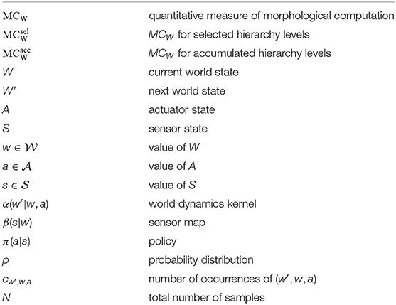
Glossary

List of Symbols

Model levels and control variables.

Morphological computation.