Quantum retrodiction in Gaussian systems and applications in optomechanics

1 Introduction

Continuous measurements (Barchielli and Gregoratti, 2009; Wiseman and Milburn, 2010; Jacobs, 2014) are a powerful tool for the preparation and control of quantum states in open systems and, as such, are of great importance for studies of fundamental physics and applications in quantum technology. Using a continuous measurement record, it is possible to track the quantum trajectory of a system in its Hilbert space in real time, as demonstrated in circuit QED systems (Weber et al., 2016; Hacohen-Gourgy and Martin, 2020), atomic ensembles (Geremia et al., 2003; Kong et al., 2020), and in optomechanics (Hofer and Hammerer, 2017) with micromechanical oscillators (Iwasawa et al., 2013; Wieczorek et al., 2015; Rossi et al., 2018; Thomas et al., 2020; Meng et al., 2022) and levitated nanoparticles (Setter et al., 2018; Liao et al., 2019; Magrini et al., 2021). Determining the conditional quantum state formally requires solving the stochastic Schrödinger or master equation (Barchielli and Gregoratti, 2009; Wiseman and Milburn, 2010; Jacobs, 2014), which is generally a daunting task. In the important case of linear quantum systems, which includes most applications in optomechanics and atomic ensembles, the integration of the Schrödinger equation simplifies the matter greatly and is actually equivalent to classical Kalman filtering (Zhang and Dong, 2022). For this reason, these well-established and powerful tools of classical estimation and control theory are finding increasing application in quantum science (Ma et al., 2022) and are becoming a well-accepted technique for preparing quantum states.

Like any measurement in quantum mechanics, continuous measurements not only determine the post-measurement state of the system but also provide information about its initial prior state. The dual use of continuous measurements for predictive preparation and retrospective analysis of quantum states—as in Figure 1—as well as their combination in what is referred to as quantum state smoothing have received considerable attention in the theoretical literature; see Chantasri et al. (2021) for a review. Retrospective state analysis and smoothing have been experimentally investigated in cavity and circuit QED (Rybarczyk et al., 2015; Tan et al., 2015; Foroozani et al., 2016; Tan et al., 2016; Tan et al., 2017), atomic ensembles (Bao et al., 2020a; Bao et al., 2020b), and optomechanics (Rossi et al., 2018; Kohler et al., 2020; Thomas et al., 2020). However, compared with quantum state preparation by filtering, the applications of these concepts for state readout appear to be less known, although they represent powerful tools for quantum state verification and tomography.

FIGURE 1

FIGURE 1. Schematic of a continuously monitored quantum system: the output of field a quantum system is combined with a strong local oscillator (LO) to perform homodyne detection from time t₀ to t₁, producing measurement record $\mathcal{Y}$. Starting from a known initial state ρ(t₀), this record can be used by integrating a stochastic master, Eq. 3, to predict the system state ${\rho }_{\mathcal{Y}}(t_1)$ conditioned on the record $\mathcal{Y}$. Alternatively, the measurement record can be used to retrodict an effect operator ${\widehat{E}}_{\mathcal{Y}}(t_0)$, cf. Eq. 36, that characterizes an effective POVM measurement on the initial state ρ(t₀).

Here, we aim to give a self-contained and accessible introduction to the theory of quantum state retrodiction based on continuous measurements and its formulation for linear quantum systems. The main equations of this theory have been derived before in the context of quantum state smoothing in (Zhang and Mølmer, 2017; Huang and Sarovar, 2018; Warszawski et al., 2020). We focus our presentation on the aspect of state retrodiction and aim to provide operational recipes for this. The general formalism is applied to optomechanical systems, for which we identify and characterize the retrodictive measurements achievable in terms of their positive operator-valued measures (POVMs). In particular, we consider the common regimes for driving the optomechanical cavity on resonance or on its red or blue mechanical sidebands and discuss the role of the local oscillator frequency in homodyne detection. In each case, we determine the realized POVM and compare it to what is achieved in state filtering in the same configuration. A main finding is that red-detuned driving in the resolved-sideband limit allows for an almost perfect quadrature measurement, which is back-action free but completely destructive. Our treatment accounts for imperfections due to thermal noise and detection inefficiencies, and it studies the requirements of quantum cooperativity for performing an efficient state readout. In particular, we determine the concrete filter functions necessary for the post-processing of the photocurrent in order to realize certain POVMs.

The remainder of the article is organized as follows: in Section 2, we recapitulate the description of conditional state preparation through continuous measurement based on stochastic master equations and the equivalent Kalman filter, emphasizing the operational interpretation of the central formulas. In close analogy, we introduce in Section 3 the formalism of retrodictive POVMs and their application to linear quantum systems, where the POVM consists of Gaussian effect operators conveniently characterized by their first and second moments. In Section 4, we illustrate the application of this formalism to the simple case of a decaying cavity. Finally, Section 5 provides a rather detailed modeling of an optomechanical system and derives the retrodictive POVMs in various parameter regimes.

2 Conditional state preparation through continuous measurements

2.1 Conditional master equation

To set the scene and introduce some notation, we start with an overview of the concept of conditional (stochastic) master equations, referring to Wiseman and Milburn (2010) and Jacobs (2014) for detailed derivations. These describe the evolution of continuously monitored quantum systems and are used to prepare conditional (or filtered) quantum states.

We consider an open quantum system governed by Hamiltonian $\widehat{H}$ and coupled to a Markovian bath via jump operator $\widehat{L}$. This gives rise to a quantum master equation (Wiseman and Milburn, 2010; Jacobs, 2014) for the system’s density operator ρ(t):

$\begin{array}{c}\hfill \mathrm{d}\rho \left(t\right)=-i\left[\widehat{H},\rho \left(t\right)\right]\mathrm{d}t+\mathcal{D}[\widehat{L}]\rho \left(t\right)\mathrm{d}t,\end{array}(1)$

with the usual Lindblad superoperator $\mathcal{D}[\widehat{L}]\rho =\widehat{L}\rho {\widehat{L}}^{†}-({\widehat{L}}^{†}\widehat{L}\rho +\rho {\widehat{L}}^{†}\widehat{L})/2$. We set ℏ = 1. The generalization to multiple jump operators is straightforward. We will designate all operators (except density operators) by caret superscripts. The increment dρ(t)≔ρ(t + dt) − ρ(t) propagates the state, by an infinitesimal amount, forward in time. Integrating this equation of motion yields a trace-preserving completely positive map ${\mathcal{N}}_{t_0,t}$ which takes an initial state ρ(t₀) to a corresponding state at a later time, $\rho (t)={\mathcal{N}}_{t_0,t}[\rho (t_0)]$ (Nielsen and Chuang, 2010).

Further information about the state can be gained by monitoring the bath to which the system is coupled (Barchielli and Gregoratti, 2009; Wiseman and Milburn, 2010; Jacobs, 2014). In that case, conditioning the state on the knowledge gained from these indirect measurements is known as filtering (Bouten et al., 2007). We only consider the case of homodyne (and later heterodyne) measurements, as we are ultimately interested in linear dynamics. Other measurement schemes, such as photon counting, would take the conditional dynamics out of this regime. A continuous homodyne detection of the outgoing mode, as sketched in Figure 1, yields a stochastic photocurrent I(t). This can be normalized, Y(t)≔I(t)/α, with some $\alpha \in \mathbb{R}$ so that, for vacuum input, its increment δY(t) = Y(t + δt) − Y(t) has the variance of white noise $\overline{\delta Y{(t)}^2}=\overline{\delta I{(t)}^2}/{\alpha }^2\equiv \delta t$, where the bar denotes an ensemble average (Authors Anonymous, 2023a). The measured signal can be decomposed into a deterministic and stochastic part as

$\left(\text{I}\right)\mathrm{d}Y\left(t\right)={⟨\widehat{C}+{\widehat{C}}^{†}⟩}_{\rho \left(t\right)}\mathrm{d}t+\mathrm{d}W\left(t\right).(2)$

Here, $\widehat{C}=\sqrt{\eta }{\mathrm{e}}^{-i\varphi }\widehat{L}$ denotes the measurement operator, which includes imperfect detection efficiency η ∈ [0, 1] and the local oscillator phase ϕ. Angled brackets denote an expectation value, ${⟨\widehat{C}⟩}_{\rho }≔\mathrm{T}\mathrm{r}\{\widehat{C}\rho \}$, and dW is a stochastic Wiener increment satisfies the Itô relation (dW)² = dt. Eq. 2 is a stochastic Itô equation (Mikosch, 1998; Gardiner, 2009) denoted by the (I) in front. Depending on the measurement results, the system satisfies the conditional master equation

$\begin{array}{cc}\hfill \left(\mathbf{I}\right)\mathrm{d}\rho \left(t\right)& =-i\left[\widehat{H},\rho \left(t\right)\right]\mathrm{d}t+\mathcal{D}[\widehat{L}]\rho \left(t\right)\mathrm{d}t\hfill \\ \hfill & +\mathcal{H}[\widehat{C}]\rho \left(t\right)\mathrm{d}W\left(t\right),\hfill \end{array}(3)$

with superoperator $\mathcal{H}[\widehat{C}]\rho ≔(\widehat{C}-{⟨\widehat{C}⟩}_{\rho })\rho +\rho ({\widehat{C}}^{†}-{⟨{\widehat{C}}^{†}⟩}_{\rho })$. Assume the system has evolved from t₀ to t₁ and produced some measurement record $\mathcal{Y}=\{Y(s),t_0\le s<t_1\}$, as depicted in Figure 1. By integrating the master equation from t₀ to t₁, we obtain a conditional (or filtered) state ${\rho }_{\mathcal{Y}}(t_1)={\mathcal{N}}_{t_0,t_1|\mathcal{Y}}[\rho (t_0)]$ dependent on the initial state ρ(t₀) and conditioned on the record $\mathcal{Y}$.

The conditional master equation Eq. (3) can be generalized to N_L Markovian baths and N_C monitored channels,

$\begin{array}{cc}\hfill \left(\mathbf{I}\right)\mathrm{d}\rho \left(t\right)& =-i\left[\widehat{H},\rho \left(t\right)\right]\mathrm{d}t+{\displaystyle \sum _{j=1}^{N_L}}\mathcal{D}[{\widehat{L}}_j]\rho \left(t\right)\mathrm{d}t\hfill \\ \hfill & +{\displaystyle \sum _{k=1}^{N_C}}\mathcal{H}[{\widehat{C}}_k]\rho \left(t\right)\mathrm{d}{W}_k\left(t\right).\hfill \end{array}(4)$

If each of the N_L decay channels is monitored, one has N_C = N_L and ${\widehat{C}}_k=\sqrt{{\eta }_k}{\mathrm{e}}^{-i{\varphi }_k}{\widehat{L}}_k$ in simple generalization of what has been introduced above for the case of a single channel. However, in general, the measurement operators ${\widehat{C}}_k$ do not necessarily correspond one-to-one to the jump operators ${\widehat{L}}_j$ as before, and we will see an example in Section 5 where, effectively, N_C > N_L. Nevertheless, since any information recorded by the observer must have previously leaked from the system, it holds that ${\sum }_j{\widehat{L}}_j^{†}{\widehat{L}}_j-{\sum }_k{\widehat{C}}_k^{†}{\widehat{C}}_k\ge 0$. The dW_j are mutually independent Wiener increments satisfying the Itô relation

$\mathrm{d}{W}_j\left(t\right)\mathrm{d}{W}_k\left(t\right)={\delta }_{jk}\mathrm{d}t,(5)$

and each dW_j is related to a corresponding homodyne measurement increment dY_j as

$\left(\mathbf{I}\right)\mathrm{d}{Y}_j\left(t\right)={⟨{\widehat{C}}_j+{\widehat{C}}_j^{†}⟩}_{\rho \left(t\right)}\mathrm{d}t+\mathrm{d}{W}_j\left(t\right).(6)$

For details and derivations of this general formalism for describing quantum dynamics conditioned on continuous homodyne detection, we refer once more to Wiseman and Milburn (2010) and Jacobs (2014).

2.2 Linear dynamics

2.2.1 Linear systems

We now apply these concepts to linear systems with Gaussian states governed by the general master equation Eq. (4). We consider a bosonic quantum system with M modes and 2M associated canonical operators ${\widehat{r}}_j$ which we collect into a vector $\widehat{\mathbf{r}}={({\widehat{r}}_j)}_{j=1,\dots ,2M}$. The ${\widehat{r}}_j$ satisfies canonical commutation relations

$i{\sigma }_{jk}≔\left[{\widehat{r}}_j,{\widehat{r}}_k\right],(7)$

giving rise to a skew-symmetric matrix $\sigma \in {\mathbb{R}}^{2M\times 2M}$. For example, the usual choice for an oscillator with M modes would be $\widehat{\mathbf{r}}={({\widehat{\mathbf{x}}}^{\mathrm{T}},{\widehat{\mathbf{p}}}^{\mathrm{T}})}^{\mathrm{T}}={({\widehat{x}}_1,\dots ,{\widehat{x}}_M,{\widehat{p}}_1,\dots ,{\widehat{p}}_M)}^{\mathrm{T}}$, which entails

$\sigma =\left(\begin{array}{cc}\hfill {\mathbb{0}}_M\hfill & \hfill {\mathbb{1}}_M\hfill \\ \hfill -{\mathbb{1}}_M\hfill & \hfill {\mathbb{0}}_M\hfill \end{array}\right).(8)$

In a linear system, the Hamiltonian is, at most, quadratic in the canonical operators while the jump and measurement operators are, at most, linear. $\widehat{H}$ can be expressed as

$\widehat{H}=\frac{1}{2}{\widehat{\mathbf{r}}}^{\mathrm{T}}H\widehat{\mathbf{r}},(9)$

with a symmetric matrix $H\in {\mathbb{R}}^{2M\times 2M}$. Without loss of generality, we assume that $\widehat{H}$ does not contain terms linear in $\widehat{\mathbf{r}}$ (Authors Anonymous, 2023e). We write the N_C linear measurement operators as

$\widehat{\mathbf{C}}=\left(A+iB\right)\widehat{\mathbf{r}},(10)$

with $A,B\in {\mathbb{R}}^{N_C\times 2M}$, and N_L jump operators as

$\widehat{\mathbf{L}}=\mathrm{\Lambda }\widehat{\mathbf{r}},(11)$

${\mathrm{\Lambda }}^{†}\mathrm{\Lambda }≕\mathrm{\Delta }+i\mathrm{\Omega },(12)$

with complex $\mathrm{\Lambda }\in {\mathbb{C}}^{N_L\times 2M}$ and $\mathrm{\Delta },\mathrm{\Omega }\in {\mathbb{R}}^{2M\times 2M}$ symmetric and skew-symmetric respectively.

2.2.2 Gaussian states

A Gaussian state ρ (Wang et al., 2007; Olivares, 2012; Weedbrook et al., 2012; Adesso et al., 2014; Genoni et al., 2016) is, by definition, any state with a Gaussian phase-space distribution. Gaussian states are fully determined by their first- and second-order cumulants (Ivan et al., 2012): a vector of means

${\mathbf{r}}_{\rho }≔{⟨\widehat{\mathbf{r}}⟩}_{\rho }:=\mathrm{T}\mathrm{r}\left\{\widehat{\mathbf{r}}\rho \right\}\in {\mathbb{R}}^{2M}(13)$

and a symmetric covariance matrix

$V_{jk}^{\rho }≔{⟨\left\{{\widehat{r}}_j-r_j^{\rho },{\widehat{r}}_k-r_k^{\rho }\right\}⟩}_{\rho }\in {\mathbb{R}}^{2M\times 2M}.(14)$

All higher-order cumulants are identically zero, so knowing r_ρ and V_ρ determines the full Wigner function of ρ and thus also ρ itself. Note that the normalization of V_ρ chosen in Eq. 14 means that diagonal elements correspond to twice the variance, such as $V_{jj}^{\rho }=2(⟨{\widehat{r}}_j^2⟩-{⟨{\widehat{r}}_j⟩}^2)$.

The assumption of a Gaussian initial state ρ(t₀) is both convenient and reasonable. Since Gaussian operators have the tremendously useful property of remaining Gaussian under linear dynamics, they are easy to work with. Additionally, consideration of only Gaussian states is justified since Gaussian measurements (Jacobs and Steck, 2006; Van Handel, 2009) and Gaussian baths (Zurek et al., 1993) tend to “Gaussify” the state of the system. Mathematically, this means that, if we start with an arbitrary initial state ρ(t₀), higher-order cumulants of order $\ge 3$ are damped by the dynamics. Depending on how slowly this damping happens, if our linear system is initially prepared in a non-Gaussian state, these higher orders may need to be taken into account—which we do in Supplementary Appendix SC5. For now, we focus only on the case of Gaussian initial states.

It is known (Barnett and Radmore, 1997; Zhang and Mølmer, 2017) that a master equation for ρ can be directly translated into differential equations for the means and covariance matrix, as detailed in Supplementary Appendix SC. One finds for a Gaussian state

$\left(\mathbf{I}\right)\mathrm{d}{\mathbf{r}}_{\rho }\left(t\right)=Q{\mathbf{r}}_{\rho }\left(t\right)\mathrm{d}t+\left(V_{\rho }\left(t\right)A^{\mathrm{T}}-\sigma B^{\mathrm{T}}\right)\mathrm{d}\mathbf{W}\left(t\right),(15)$

with the drift matrix

$Q≔\sigma \left(H+\mathrm{\Omega }\right),(16)$

comprising unitary and dissipative terms. If we reintroduce the homodyne signal actually measured,

$\left(\mathbf{I}\right)\mathrm{d}\mathbf{Y}\left(t\right)=2A{\mathbf{r}}_{\rho }\left(t\right)\mathrm{d}t+\mathrm{d}\mathbf{W}\left(t\right),(17)$

we can write

$\left(\mathbf{I}\right)\mathrm{d}{\mathbf{r}}_{\rho }\left(t\right)=M_{\rho }\left(t\right){\mathbf{r}}_{\rho }\left(t\right)\mathrm{d}t+\left(V_{\rho }\left(t\right)A^{\mathrm{T}}-\sigma B^{\mathrm{T}}\right)\mathrm{d}\mathbf{Y}\left(t\right),(18)$

with the conditional drift matrix

$M_{\rho }\left(t\right)≔Q+2\sigma B^{\mathrm{T}}A-2V_{\rho }\left(t\right)A^{\mathrm{T}}A.(19)$

In Eq. 18, the measurement current dY(t) enters the evolution of the conditional means only through multiplication with the measurement matrices A and B. Hence, reducing the detection efficiency corresponding to A, B → 0 causes the stochastic increment to disappear as it should. Note that the covariance matrix V_ρ(t) twice enters Eq. 18, once through the drift matrix M_ρ(t) and once directly coupled to dY(t). The latter term has the effect that a large variance, which corresponds to great uncertainty about the state, boosts the effect that each bit of gathered information has on the evolution of the conditional means.

The covariance matrix satisfies the deterministic equation

$\begin{array}{cc}\hfill \frac{\mathrm{d}{V}_{\rho }\left(t\right)}{\mathrm{d}t}& =M_{\rho }\left(t\right)V_{\rho }\left(t\right)+V_{\rho }\left(t\right)M_{\rho }^{\mathrm{T}}\left(t\right)\hfill \\ \hfill & +D+2V_{\rho }\left(t\right)A^{\mathrm{T}}A{V}_{\rho }\left(t\right),\hfill \end{array}(20)$

with diffusion matrix

$D≔2\sigma \left(\mathrm{\Delta }-B^{\mathrm{T}}B\right){\sigma }^{\mathrm{T}}.(21)$

The evolution of V_ρ(t) is independent of the means r_ρ(t) or any other cumulants, which is a peculiarity of Gaussian dynamics. However, while it is independent of the measurement record and not a stochastic equation, it does depend on the measurement device through matrices A, B. This is reasonable, since the information that is gained from observations of the system conditions the state, thus reducing its uncertainty.

In the following, we assume stable dynamics, which makes the covariance matrix collapse to some steady state matrix $V_{\rho }(t)\to V_{\rho }^{\infty }$ asymptotically for t → ∞ from any initial V_ρ(t₀). We find $V_{\rho }^{\infty }$ by solving the Riccati equation ${\dot{V}}_{\rho }=0$ which implies

$M_{\rho }^{\infty }{V}_{\rho }^{\infty }+V_{\rho }^{\infty }{\left(M_{\rho }^{\infty }\right)}^{\mathrm{T}}=-D-2V_{\rho }^{\infty }{A}^{\mathrm{T}}A{V}_{\rho }^{\infty },(22)$

where $M_{\rho }^{\infty }$ is just M_ρ(t) with $V_{\rho }(t)\mapsto V_{\rho }^{\infty }$. The right-hand side is negative definite and the covariance matrix is positive definite for proper quantum states, so $M_{\rho }^{\infty }$ only has eigenvalues with negative real part. Now if the experiment has been running sufficiently long, we can simply plug $V_{\rho }^{\infty }$ and $M_{\rho }^{\infty }$ into Eq. 18 to find the evolution of the means:

$\begin{array}{ll}\hfill \left(\mathbf{I}\right){\mathbf{r}}_{\rho }\left(t\right)& ={\mathrm{e}}^{\left(t-t_0\right)M_{\rho }^{\infty }}{\mathbf{r}}_{\rho }\left(t_0\right)\hfill \\ \hfill & +{\int }_{t_0}^t{\mathrm{e}}^{\left(t-\tau \right)M_{\rho }^{\infty }}\left(V_{\rho }^{\infty }{A}^{\mathrm{T}}-\sigma B^{\mathrm{T}}\right)\mathrm{d}\mathbf{Y}\left(\tau \right).\hfill \end{array}(23)$

Because $M_{\rho }^{\infty }$ is stable (all eigenvalues have non-positive real parts), we see that the initial condition r_ρ(t₀) is damped exponentially, as is the integrand in the second line.

Here, we see that the means (and thus the whole state) do not depend on the entire continuous measurement record $\mathcal{Y}$ as such, but only on the Itô-integral in the second line of Eq. 23, which is a simple vector of 2M real numbers for a system composed of M subsystems. Thus, the integral kernel ${\mathrm{e}}^{M_{\rho }^{\infty }(t-\tau )}\left(V_{\rho }^{\infty }{A}^{\mathrm{T}}-\sigma B^{\mathrm{T}}\right)$ actually picks out a set of 2M temporal modes of the monitored fields. Each of these (not necessarily orthogonal) modes of the light fields provides an estimate for one of the 2M phase space variables of the system. We will elaborate on this aspect further in Section 2 C 2. For the particular case of a freely decaying monitored cavity, this fact was already pointed out by Wiseman (1996); in Section 4, we will treat this cavity as an illustrative example of the formalism developed here, reproducing the results of Wiseman (1996).

2.3 Interpretation and discussion

2.3.1 Conditional quantum states

We now want to remind the reader of how the conditional Gaussian quantum state should be interpreted and what its preparation via continuous measurements means from an operational perspective.

The means r_ρ(t) and covariance matrix V_ρ(t) determined from Eqs 18 and (20) fully determine the density matrix for the conditional state. It is instructive to note that the Gaussian density matrix is always of the form (Giedke, 2001; Fiurášek and Mišta, 2007)

$\rho \left(t\right)\propto \widehat{D}\left({\mathbf{r}}_{\rho }\left(t\right)\right)\exp \left[-{\widehat{\mathbf{r}}}^{\mathrm{T}}{\mathrm{\Gamma }}_{\rho }\left(t\right)\widehat{\mathbf{r}}\right]{\widehat{D}}^{†}\left({\mathbf{r}}_{\rho }\left(t\right)\right).(24)$

Here, $\widehat{D}(\mathbf{q})=\exp (-i\mathbf{q}\sigma \widehat{\mathbf{r}})$ is a displacement operator in phase space and the matrix Γ_ρ(t) is a simple functional of the covariance matrix (Authors Anonymous, 2023b). The shape of the Gaussian wave packet in phase space is determined by the middle term on the right-hand side, which evolves deterministically and is independent of the measurement results. The wave packet’s position in phase space is set by the displacement operators and depends on the photocurrent via Eq. 23.

Therefore, predicting a conditional quantum state based on a continuous measurement during time interval [t₀, t] starting from a known Gaussian initial state simply means calculating the means according to Eq. 23. Knowing those numbers, the prediction is that a hypothetical projective measurement of canonical operators at time t will give results with these same averages, and second moments according to the covariance matrix V_ρ(t) which depends only on the initial condition. Statistics of any other measurement can be determined from Eq. 24. For stable dynamics, dependencies on initial conditions will disappear in the long run, and the covariance matrix will become time-independent. The wave packet will then have a fixed shape and undergo stochastic motion in phase space with positions known from the photocurrent.

The quality of the conditional preparation can be judged from the purity $\mathcal{P}(\rho )=\mathrm{T}\mathrm{r}\{{\rho }^2\}\le 1$ of the conditional state. It tells us how close it is to a pure state and thus quantifies the amount of classical uncertainty in ρ. For a Gaussian state with M modes, it is given by (Paris et al., 2003)

$\mathcal{P}\left(\rho \right)=1/\sqrt{\det \left(V_{\rho }\right)}.(25)$

Unobserved dissipation tends to reduce the purity, while monitoring the dynamics and conditioning the state increases the purity. Ideally, perfect detection allows preparation of pure states, which are the only states with $\mathcal{P}(\rho )=1$. The bound $\mathcal{P}\le 1$ implies det(V_ρ) ≥ 1, which is also imposed by Heisenberg’s uncertainty relation. We briefly recall prototypical pure Gaussian states of a single mode. Coherent states |α⟩ have equal variances V_xx = V_pp = 1 and vanishing covariance. The vacuum |0⟩ is a special coherent state with vanishing means. Squeezed states (Barnett and Radmore, 1997) have the variance in one quadrature reduced below shot noise—below 1 (the variance of vacuum). The conjugate quadrature is then necessarily anti-squeezed to satisfy Heisenberg’s uncertainty relation. An important class of non-pure Gaussian states is thermal states. These have vanishing covariance and equal variance $V_{xx}=V_{pp}=2\bar{n}+1$, where $\bar{n}\ge 0$ is the mean number of excitations. Importantly, $\mathcal{P}=1/(2\bar{n}+1)$ decreases as $\bar{n}$ grows.

2.3.2 Mode functions

We mentioned at the end of Section 2 B 2 that the kernels in the forward and backward integrals of the means in Eq. 23 and Eq. 46 each select sets of temporal modes. Recall that the means ${\mathbf{r}}_{\rho }(t)={(r_j(t))}_{j=1,\dots ,2M}$ in Eq. 23 depend on the measurement currents $\mathbf{Y}(\tau )={(Y_k(\tau ))}_{k=1,\dots ,N_C}$ only through integration with respect to the functions

$f_{jk}^{\rho }\left(t,\tau \right)≔{\left[{\mathrm{e}}^{\left(t-\tau \right)M_{\rho }^{\infty }}\left(V_{\rho }^{\infty }{A}^{\mathrm{T}}-\sigma B^{\mathrm{T}}\right)\right]}_{jk}.(26)$

Each (unnormalized) temporal mode function $f_{jk}^{\rho }(t,\tau )$ is integrated with a corresponding signal Y_k(τ),

$X_j\left(t\right)≔{\int }_{t_0}^t{f}_{jk}^{\rho }\left(t,\tau \right)\mathrm{d}{Y}_k\left(\tau \right),(27)$

to enter the evolution of r_j(t). The interpretation of this is as follows: the time integral of extracts from the continuous quadrature-measurement current Y_k(τ) a single number X_j(t), which can be considered the result of the measurement of the quadrature of temporal modes with envelope functions $f_{jk}^{\rho }(t,\tau )$.

3 State verification using retrodictive POVMs

3.1 Retrodictive POVMs

In the previous section, we have seen how to use continuous monitoring to prepare conditional states (filtering). We will now show how to interpret the measurement record instead as an instantaneous POVM (Nielsen and Chuang, 2010; Wiseman and Milburn, 2010; Jacobs, 2014). To fully appreciate this result, let us first remind the reader about POVMs and general measurements in quantum mechanics.

3.1.1 Positive operator-valued measures

A general measurement of a given quantum state ρ is always composed of i) possible measurement outcomes $x\in \mathcal{X}$, ii) probabilities for those outcomes to occur P(x|ρ), and iii) the effect that obtaining some outcome x has on the system—the post-measurement state ${\rho }_x\propto {\widehat{M}}_x\rho {\widehat{M}}_x^{†}$ where ${\widehat{M}}_x$ incorporates the measurement back action on the state. The probability for a particular x to be measured is given by

$P\left(x|\rho \right)=\mathrm{T}\mathrm{r}\left\{{\widehat{M}}_x\rho {\widehat{M}}_x^{†}\right\}=\mathrm{T}\mathrm{r}\left\{{\widehat{M}}_x^{†}{\widehat{M}}_x\rho \right\}=\mathrm{T}\mathrm{r}\left\{{\widehat{E}}_x\rho \right\}(28)$

with the positive effect operator ${\widehat{E}}_x≔{\widehat{M}}_x^{†}{\widehat{M}}_x$. Because ∑_xP(x|ρ) = 1 must hold for any ρ, the operators ${\widehat{E}}_x$ must resolve the identity ${\sum }_x{\widehat{E}}_x=\widehat{1}$. Without reference to the ${\widehat{M}}_x$, any collection of positive self-adjoint operators $\{{\widehat{E}}_x,x\in \mathcal{X}\}$ which resolve the identity is called a POVM.

3.1.2 Continuous monitoring as POVM measurement

To see how to reinterpret the measurement record, we again consider the simple system governed by the master Equation 3 and an evolution from t₀ to t₁ that produced some record $\mathcal{Y}=\{Y(s),t_0\le s<t_1\}$. Note that Eq. 3 is nonlinear in ρ in order to yield a trace-preserving map ${\mathcal{N}}_{t_0,t_1|\mathcal{Y}}$. If, instead, we consider the linear equation (Wiseman, 1996)

$\begin{array}{cc}\hfill \left(\mathbf{I}\right)\mathrm{d}\tilde{\rho }\left(t\right)& =-i\left[\widehat{H},\tilde{\rho }\left(t\right)\right]\mathrm{d}t+\mathcal{D}[\widehat{L}]\tilde{\rho }\left(t\right)\mathrm{d}t\hfill \\ \hfill & +\left(\widehat{C}\tilde{\rho }\left(t\right)+\tilde{\rho }\left(t\right){\widehat{C}}^{†}\right)\mathrm{d}Y\left(t\right),\hfill \end{array}(29)$

we find that it generates equivalent but non-trace-preserving dynamics,

${\tilde{\rho }}_{\mathcal{Y}}\left(t_1\right)={\tilde{\mathcal{N}}}_{t_0,t_1|\mathcal{Y}}\left[\rho \left(t_0\right)\right],(30)$

denoted by a tilde. The trace of the conditional state now carries additional information: the probability for $\mathcal{Y}$ to have occurred given an initial ρ(t₀),

$P\left(\mathcal{Y}|\rho \left(t_0\right)\right)=\mathrm{T}\mathrm{r}\left\{{\tilde{\rho }}_{\mathcal{Y}}\left(t_1\right)\right\}.(31)$

If we plug Eq. 30 into this expression and include an identity operator $\widehat{1}$, we can write

$P\left(\mathcal{Y}|\rho \left(t_0\right)\right)=\mathrm{T}\mathrm{r}\left\{\widehat{1}{\tilde{\mathcal{N}}}_{t_0,t_1|\mathcal{Y}}\left[\rho \left(t_0\right)\right]\right\},(32)$

$=\mathrm{T}\mathrm{r}\left\{{\tilde{\mathcal{N}}}_{t_0,t_1|\mathcal{Y}}^{†}\left[\widehat{1}\right]\rho \left(t_0\right)\right\},(33)$

where ${\tilde{\mathcal{N}}}_{t_0,t_1|\mathcal{Y}}^{†}$ is the Hilbert–Schmidt adjoint channel of ${\tilde{\mathcal{N}}}_{t_0,t_1|\mathcal{Y}}$ that acts on $\widehat{1}$. We now define

${\widehat{E}}_{\mathcal{Y}}\left(t_0\right)≔{\tilde{\mathcal{N}}}_{t_0,t_1|\mathcal{Y}}^{†}\left[\widehat{1}\right],(34)$

which will play a crucial role throughout this article. With this definition, Eq. 33 can be rewritten as

$P\left(\mathcal{Y}|\rho \left(t_0\right)\right)=\mathrm{T}\mathrm{r}\left\{{\widehat{E}}_{\mathcal{Y}}\left(t_0\right)\rho \left(t_0\right)\right\}.(35)$

A comparison of Eq. 35 with Eq. 28 shows that $\{{\widehat{E}}_{\mathcal{Y}}(t_0),\mathcal{Y}\in \mathfrak{Y}\}$ indeed constitutes a POVM on the initial state ρ(t₀). Here, the “outcomes” $x\equiv \mathcal{Y}\in \mathfrak{Y}$ comprise all possible records one could observe, and ${\sum }_{Y\in \mathcal{Y}}P(\mathcal{Y}|\rho (t_0))=1$ because the sum corresponds to averaging over (i. e., ignoring) the observations, which yields the unconditional trace-preserving evolution (1). As in filtering, we will later show that the effect operators actually only depend on certain weighted integrals of the measurement record $\mathcal{Y}$ and not on the whole continuous record as such.

3.2 Backward effect equation

Just as the conditional quantum state, the effect operators ${\widehat{E}}_{\mathcal{Y}}(t)$ themselves can be considered dynamic quantities that obey a certain (stochastic) equation of motion. In open but unobserved systems, Barnett et al. (2000), Barnett et al. (2001), and Pegg et al. (2002) derived a deterministic differential equation describing the propagation backward in time of effect operators to yield effective POVMs at past times. Tsang (2009a), Tsang (2009b), Tsang, (2010), Gammelmark et al. (2013), and Zhang and Mølmer (2017) incorporated continuous observations into Bayesian updates of past measurement results, which (arguably, see Guevara and Wiseman (2015)) extends classical smoothing to the quantum domain and results in a stochastic differential equation for ${\widehat{E}}_{\mathcal{Y}}(t)$.

For a given system dynamics, the effect operators are backpropagated by a channel adjoint to that of the state. More specifically, for continuously monitored systems governed by conditional master Equation 29, the adjoint conditional effect equation, which takes some effect operator $\widehat{E}(t)$ from the future to the past reads (Tsang, 2009a; Tsang, 2009b; Gammelmark et al., 2013)

$\begin{array}{cc}\hfill \left(\mathbf{BI}\right)-\mathrm{d}\widehat{E}\left(t\right)& ≔\widehat{E}\left(t-\mathrm{d}t\right)-\widehat{E}\left(t\right)\hfill \\ \hfill & =i\left[\widehat{H},\widehat{E}\left(t\right)\right]\mathrm{d}t+{\mathcal{D}}^{†}[\widehat{L}]\widehat{E}\left(t\right)\mathrm{d}t\hfill \\ \hfill & +\left({\widehat{C}}^{†}\widehat{E}\left(t\right)+\widehat{E}\left(t\right)\widehat{C}\right)\mathrm{d}Y\left(t\right),\hfill \end{array}(36)$

with adjoint Lindblad superoperator ${\mathcal{D}}^{†}[\widehat{L}]\widehat{E}≔{\widehat{L}}^{†}\widehat{E}\widehat{L}-\frac{1}{2}{\widehat{L}}^{†}\widehat{L}\widehat{E}-\frac{1}{2}\widehat{E}{\widehat{L}}^{†}\widehat{L}$. The (BI) indicates that the equation should be treated as a backward Itô equation. In Supplementary Appendix SA, we give a detailed derivation of this equation and comment further on its interpretation as a differential equation for propagation backward in time. Note that we defined the increment $\mathrm{d}\widehat{E}$ with an explicit minus sign. This differs from the convention of Gammelmark et al. (2013) and Zhang and Mølmer (2017) but follows the convention of Tsang (Tsang, 2009a; Tsang, 2009b).

Comparing the effect Equation 36 to the forward master Equation 29, we observe the following differences. The sign of the Hamiltonian changes, which we expect from the usual time-reversal in closed systems. The Lindblad superoperator $\mathcal{D}$ is replaced by its adjoint ${\mathcal{D}}^{†}$, which is no longer trace-preserving but vanishes when applied to the identity. The measurement operator $\widehat{C}$ is replaced by its adjoint.

Solving Eq. 36 for $\widehat{E}(t)$ for t ≤ t₁ requires a certain final condition $\widehat{E}(t_1)$. We have motivated the definition (34) of the effect operator by means of the final condition $\widehat{E}(t_1)=\widehat{1}$. This can be interpreted as describing a situation where, at time t₁, a certain $\{{\widehat{E}}_x,x\in \mathcal{X}\}$ is performed on the system, but the outcome x is not registered. If the outcome x is registered and we want to describe a dynamics post-selected on it, we need to replace the identity in Eq. 33 by ${\widehat{E}}_x(t_1)$ to obtain an effective ${\widehat{E}}_{x,\mathcal{Y}}(t_0)$. This general observation-assisted back-propagation is what we refer to as retrodiction. It is remarkable that a non-trivial POVM can also be retrodicted starting from the trivial effect operator $\widehat{E}(t_1)=\widehat{1}$ using nothing but knowledge of the system’s dynamics and continuous observations. In fact, in many relevant cases the final condition on $\widehat{E}$ will be damped out in the long run, just as initial conditions for the forward propagated density matrix become irrelevant for stable dynamics. This point will be addressed more rigorously further below.

The unnormalized effect equation generalizing Eq. 36 to multiple observed and unobserved channels reads

$\begin{array}{cc}\hfill \left(\mathbf{BI}\right)-\mathrm{d}\widehat{E}\left(t\right)& =i\left[\widehat{H},\widehat{E}\left(t\right)\right]\mathrm{d}t+{\displaystyle \sum _{j=1}^{N_L}}{\mathcal{D}}^{†}\left[{\widehat{L}}_j\right]\widehat{E}\left(t\right)\mathrm{d}t\hfill \\ \hfill & +{\displaystyle \sum _{k=1}^{N_C}}\left({\widehat{C}}_k^{†}\widehat{E}\left(t\right)+\widehat{E}\left(t\right){\widehat{C}}_k\right)\mathrm{d}{Y}_k\left(t\right).\hfill \end{array}(37)$

Since we only consider conditional dynamics from now on, we will drop the subscript $\mathcal{Y}$ and remember that both ρ and $\widehat{E}$ depend on respective parts of the monitoring record.

3.3 Linear dynamics and Gaussian POVMs

As in Section 2 B, we focus our approach on linear systems. Like density operators, we can represent effect operators in terms of phase space distributions, which allow us to translate the effect equation into differential equations for the cumulants. We must be more careful with the definition of statistical quantities, as $\widehat{E}$ does not have unit trace (or may not be trace class at all). For example, the means and covariance matrix are given by

$r_j^E≔\langle {\widehat{r}}_j{\rangle }_E≔\frac{\mathrm{T}\mathrm{r}\left\{{\widehat{r}}_j\widehat{E}\right\}}{\mathrm{T}\mathrm{r}\left\{\widehat{E}\right\}},(38)$

$V_{jk}^E=\langle \left\{{\widehat{r}}_j-r_j^E,{\widehat{r}}_k-r_k^E\right\}{\rangle }_E,(39)$

where the expectation value ⟨⋅⟩_E is explicitly normalized and is defined as long as $\mathrm{T}\mathrm{r}\{\widehat{E}\}$ exists.

Gaussian effect operators and their time dynamics have been treated recently by Zhang and Mølmer (2017), Huang and Sarovar (2018), and Warszawski et al. (2020). Since we aim to keep our treatment self-contained, we reproduce a number of the results (in particular on the Gaussian equations of motion of the effect operator) presented there. Our derivation and presentation complements these previous ones with further details and background. In particular, it was not apparent to us if the restriction to Gaussian effect operators is justified as it is for quantum states (cf. the discussion in Section 2 B 2). In Supplementary Appendix SC7, we consider the evolution of general effect operators and show that it is very similar to that of general quantum states. Hence, a notion of backward stability analogous to that of quantum states can be applied.

To obtain the evolution of the means and covariance matrix associated with $\widehat{E}$ from the corresponding equations for r_ρ and V_ρ, let us rewrite the effect Equation 37 as

$\begin{array}{cc}\hfill \left(\mathbf{BI}\right)-\mathrm{d}\widehat{E}\left(t\right)& =-i\left[-\widehat{H},\widehat{E}\left(t\right)\right]\mathrm{d}t+{\displaystyle \sum _{j=1}^{N_L}}\mathcal{D}\left[{\widehat{L}}_j\right]\widehat{E}\left(t\right)\hfill \\ \hfill & +{\displaystyle \sum _{j=1}^{N_L}}\left({\widehat{L}}_j^{†}\widehat{E}\left(t\right){\widehat{L}}_j-{\widehat{L}}_j\widehat{E}\left(t\right){\widehat{L}}_j^{†}\right)\mathrm{d}t\hfill \\ \hfill & +{\displaystyle \sum _{k=1}^{N_C}}\left({\widehat{C}}_k^{†}\widehat{E}\left(t\right)+\widehat{E}\left(t\right){\widehat{C}}_k\right)\mathrm{d}{Y}_k\left(t\right),\hfill \end{array}(40)$

where the second line compensates for the replacement of ${\mathcal{D}}^{†}$ by $\mathcal{D}$. We see that this equation is structurally very similar to the unnormalized master Equation 4, so Eqs 18 and 20 for dr_ρ and ${\dot{V}}_{\rho }$ serve as a good starting point with the following changes: i) time-reversal requires they be treated as backward Itô equations (cf. Supplementary Appendix SB); ii) the sign flip of $\widehat{H}$ causes H↦ − H and replaces the measurement operators ${\widehat{C}}_k$ by their adjoint entails B↦ − B; iii) working out the change stemming from the sandwich terms in the second line, we find in Supplementary Appendix SC7 that it contributes terms −2σΩr_E and $-\sigma \mathrm{\Omega }{V}_E-{(\sigma \mathrm{\Omega }{V}_E)}^{\mathrm{T}}$ to the evolution of the means and covariance matrix, respectively. Together with H↦ − H, this simply changes the sign of the unconditional drift matrix Q↦ − Q. Hence, the backward Itô equation for the means reads

$\begin{array}{cc}\hfill & \left(\mathbf{BI}\right)-\mathrm{d}{\mathbf{r}}_E\left(t\right)≔{\mathbf{r}}_E\left(t-\mathrm{d}t\right)-{\mathbf{r}}_E\left(t\right)\hfill \\ \hfill & =M_E\left(t\right){\mathbf{r}}_E\left(t\right)\mathrm{d}t+\left(2V_E\left(t\right)A^{\mathrm{T}}+\sigma B^{\mathrm{T}}\right)\mathrm{d}\mathbf{Y}\left(t\right),\hfill \end{array}(41)$

with the conditional backward drift matrix

$M_E\left(t\right)≔-Q-2\sigma B^{\mathrm{T}}A-2V_E\left(t\right)A^{\mathrm{T}}A.(42)$

The deterministic backward Riccati equation for the covariance matrix is similar to Eq. 20,

$\begin{array}{cc}\hfill -\frac{\mathrm{d}{V}_E\left(t\right)}{\mathrm{d}t}& ≔V_E\left(t-\mathrm{d}t\right)-V_E\left(t\right)\hfill \\ \hfill & =M_E\left(t\right)V_E\left(t\right)+V_E\left(t\right)M_E^{\mathrm{T}}\left(t\right)\hfill \\ \hfill & +D-2V_E\left(t\right)A^{\mathrm{T}}A{V}_E\left(t\right),\hfill \end{array}(43)$

and clearly shows the importance of continuous observations for retrodiction. Without observations (i. e., when A = B = 0), the drift matrices would be equal up to sign M_ρ(t) = −M_E(t) = Q. At the same time, the quadratic Riccati equations for the respective covariance matrices would turn into linear Lyapunov equations. Assuming stable forward dynamics with a positive steady state solution $V_{\rho }^{\infty }>0$ of Eq. 22,

$Q{V}_{\rho }^{\infty }+V_{\rho }^{\infty }{Q}^{\mathrm{T}}=-D(44)$

would preclude stable backward dynamics: there cannot simultaneously be a positive asymptotic covariance matrix $V_E^{\infty }>0$ for t → −∞ that satisfies

$-Q{V}_E^{\infty }-V_E^{\infty }{Q}^{\mathrm{T}}=-D.(45)$

Only the presence of a sufficiently large quadratic A^TA-term in Eq. 43, corresponding to sufficiently efficient observations, allows us to find an asymptotic solution $V_E^{\infty }>0$. Analogous to Eq. 22, this implies an asymptotic drift matrix $M_E^{\infty }$ whose eigenvalues have negative real parts.

Assuming stable backward dynamics that make any Gaussian effect operator with V_E(t₁) collapse to $V_E^{\infty }$ as t → −∞, we can plug the asymptotic solution $V_E^{\infty }$ into the equation for the means. As with the forward solution in Eq. 23, we find

$\begin{array}{ll}\hfill \left(\text{BI}\right){\mathbf{r}}_E\left(t\right)& ={\mathrm{e}}^{\left(t_1-t\right)M_E^{\infty }}{\mathbf{r}}_E\left(t_1\right)\hfill \\ \hfill & +{\int }_t^{t_1}{\mathrm{e}}^{\left(\tau -t\right)M_E^{\infty }}\left(V_E^{\infty }{A}^{\mathrm{T}}+\sigma B^{\mathrm{T}}\right)\mathrm{d}\mathbf{Y}\left(\tau \right),\hfill \end{array}(46)$

where the integral is a backward Itô integral as explained in Supplementary Appendix SB. The negative eigenvalues of $M_E^{\infty }$ again cause exponential damping of the final condition r_E(t₁) and of the integrand, which picks out a different set of modes compared to the forward integral in Eq. 23 (cf. Section 2 C 2).

3.4 Interpretation of retrodictive POVMs

Analogous to Eq. 24, the POVM realized at time t in retrodiction based on continuous homodyne detection during some time interval [t, t₁] can be written as

$\left\{\widehat{D}\left({\mathbf{r}}_E\left(t\right)\right){\widehat{E}}_0\left(t\right){\widehat{D}}^{†}\left({\mathbf{r}}_E\left(t\right)\right)\right\}.(47)$

Here, ${\widehat{E}}_0(t)=\exp \left[-{\widehat{\mathbf{r}}}^{\mathrm{T}}{\mathrm{\Gamma }}_E(t)\widehat{\mathbf{r}}\right]$ is independent of the means, since Γ_E(t) is determined by the covariance matrix V_E(t) as explained in Eq. 24. Means r_E(t) and covariance matrices V_E(t) are determined by (41) and 43. The POVM elements all correspond to displaced versions of the operator ${\widehat{E}}_0(t)$. The shape of ${\widehat{E}}_0(t)$ determines the resolution in phase space achieved by the POVM in retrodiction. It is again useful to consider the purity of a Gaussian effect operator $\widehat{E}$ with covariance matrix V_E, which is computed as in Eq. 25. Unit purity means that the given POVM actually corresponds to projections onto pure states, constituting a quantum-limited measurement. Pure POVM elements with equal variances then indicate a projection onto coherent states, which corresponds to a heterodyne measurement of both quadratures (Wiseman and Milburn, 2010), that is, $\left\{|\alpha \rangle \langle \alpha |/\pi \right\}$. Asymmetric variances, on the other hand, indicate squeezed projectors that correspond, in the ideal limit of infinite squeezing, to a measurement of only one quadrature, {|x⟩⟨x|}, where |x⟩ denotes a quadrature eigenstate.

Reduced purity means additional uncertainty and thus lower resolution of the measurement. We will see in the examples in Sections 4 and 5 that the purity of retrodicted effect operators decreases quickly when the detection efficiency is low or when there is coupling to unobserved baths. Quite generally, for systems subject to continuous time measurements with a measurement rate Γ (including losses) competing with other decoherence processes happening at rate γ, the dynamics of both conditional density and effect matrix crucially depend on a quantum cooperativity parameter C_q = Γ/γ. The regime C_q > 1 signifies the possibility of producing quantum-limited POVMs in retrodiction just as it allows pure conditional quantum states in prediction. In Section 5, we will prove this statement in great detail for continuous measurements on optomechanical systems.

While it is possible to perform quantum limited POVMs corresponding to projections on pure states, this cannot be used as a means of preparing pure quantum states. The “collapsed” posterior state is physically not realized since retrodictive POVMs are destructive: once all information necessary for realizing the POVM has been gathered, the system’s state has already evolved into something different, the best description of which is just the conditional quantum state. It does not make sense to consider the posterior state after the measurement just as it is useless to ask for the state of a photon after photo-detection.

Repeated measurement of a POVM (47) on identically prepared systems in state ρ₀ will map out the probability distribution

$P\left(\mathbf{r}|{\rho }_0\right)=\mathrm{T}\mathrm{r}\left\{D\left(\mathbf{r}\right){\widehat{E}}_0{D}^{†}\left(\mathbf{r}\right){\rho }_0\right\}.$

This is the information on the state ρ₀, which is directly accessible via retrodictive POVMs. Other relevant aspects regarding the quantum state may be inferred from such information, possibly collected for different POVMs by changing the dynamics—and with it, the equations of motion for $\widehat{E}(t)$—of the system.

One may, for example, be interested in reconstructing the density matrix ρ₀ itself, which corresponds to the problem of quantum state tomography. Recapitulating the methods available to perform this task is beyond the scope of this article, and we refer to the literature in this field (Paris and Řeháček, 2004; Lvovsky and Raymer, 2009). We just state two particularly simple cases where the heterodyne POVM directly provides the Mandel Q-function of the quantum state, $Q(\alpha )=\left.⟨\alpha \right|{\rho }_0\left|\alpha \right.⟩$. If ρ₀ was known to be Gaussian, this POVM would directly give the correct means and (co)variances with one unit of added quantum noise in each quadrature. A POVM corresponding to an infinitely squeezed state will give direct access to the marginal distribution in the respective quadrature $\left.⟨x\right|{\rho }_0\left|x\right.⟩$.

It is worth emphasizing that the Gaussian POVMs realized by the linear dynamics considered here may well be applied to non-Gaussian states. No assumption of the initial state ρ₀ went into the derivation of the equations of motions (41) and (43) for the Gaussian operator $\widehat{E}(t)$. Provided the measurement delivers sufficient resolution in phase space, the tools of retrodictive Gaussian POVMs can therefore be used for verification of non-Gaussian states which have been created initially by some different means (of course, those initial states cannot emerge as conditional states from Gaussian dynamics and homodyne detections alone.) Along these lines, the preparation and verification of Fock states in macroscopic mechanical oscillators have been discussed by Khalili et al. (2010)—see also Miao et al. (2010).

4 Basic examples

In this section, we consider two basic but illustrative examples of the formalism developed so far; these will provide a firm basis for the more serious application to optomechanical systems in Section 5.

4.1 Monitoring a decaying cavity

Let us start with the simple example of a decaying cavity undergoing homodyne detection (Figure 2). This example was used by Wiseman (1996) to illustrate the interpretation of quantum trajectories in measurement theory as retrodictive POVM elements. Using operator algebra, he showed that, with an ideal detector and infinite observation time, one can perform a projective measurement of the initial state of the cavity onto a quadrature eigenstate. Using the formalism developed in the previous sections, we will treat the same setup here for homodyne detection with efficiency η. For ideal detection η → 1, we recover the result of Wiseman.

FIGURE 2

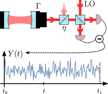
FIGURE 2. Schematic of a freely decaying cavity monitored from time t₀ to t₁. Light leaving the cavity at rate Γ is superposed on a balanced beam-splitter with a strong local oscillator (LO). Two photodetectors monitor the output ports and their photocurrents are subtracted to yield a time-continuous homodyne measurement signal Y(t). Imperfect detection is modeled as photon loss induced by a second beam-splitter which only transmits a fraction η of the signal light.

4.1.1 Conditional state evolution

We consider an ideal freely damped cavity with decay rate Γ. The output is mixed with a strong local oscillator with adjustable relative phase ϕ to perform homodyne detection with efficiency η ∈ [0, 1]. For later reference, we first study the corresponding stochastic master equation for the conditional state of the intra-cavity field (Wiseman, 1996). In a frame rotating at the cavity frequency, this is

$\left(\mathbf{I}\right)\mathrm{d}\rho \left(t\right)=\mathrm{\Gamma }\mathcal{D}[\widehat{a}]\rho \left(t\right)\mathrm{d}t+\sqrt{\eta \mathrm{\Gamma }}\mathcal{H}[{\mathrm{e}}^{-i\varphi }\widehat{a}]\rho \left(t\right)\mathrm{d}W\left(t\right),(48)$

where ${\widehat{a}}^{†},\widehat{a}$ are the cavity creation and annihilation operators (CAOs). The canonical quadrature operators are $\widehat{x}=(\widehat{a}+{\widehat{a}}^{†})/\sqrt{2}$ and $\widehat{p}=-i(\widehat{a}-{\widehat{a}}^{†})/\sqrt{2}$ which we collect into a vector $\widehat{\mathbf{r}}={\left[\begin{array}{cc}\hfill \widehat{x}\hfill & \hfill \widehat{p}\hfill \end{array}\right]}^{\mathrm{T}}$. The Wiener increment dW(t) is then related to the detector output dY(t) as

$\mathrm{d}Y\left(t\right)=\sqrt{2\eta \mathrm{\Gamma }}{⟨{\widehat{x}}_{\varphi }⟩}_{\rho \left(t\right)}\mathrm{d}t+\mathrm{d}W\left(t\right),(49)$

with ${\widehat{x}}_{\varphi }≔\cos (\varphi )\widehat{x}+\sin (\varphi )\widehat{p}$. Due to the symmetry of the problem, we choose ϕ = 0 without loss of generality, observing only the $\widehat{x}$-quadrature of the cavity.

Spelling out Eqs 15 and (20) for dr_ρ and ${\dot{V}}_{\rho }$, we find

$\left(\mathbf{I}\right)\mathrm{d}{x}_{\rho }\left(t\right)=-\frac{\mathrm{\Gamma }}{2}{x}_{\rho }\mathrm{d}t+\sqrt{\frac{\eta \mathrm{\Gamma }}{2}}\left(V_{xx}^{\rho }\left(t\right)-1\right)\mathrm{d}W\left(t\right),(\mathrm{50a})$

$\left(\mathbf{I}\right)\mathrm{d}{p}_{\rho }\left(t\right)=-\frac{\mathrm{\Gamma }}{2}{p}_{\rho }\mathrm{d}t+\sqrt{\frac{\eta \mathrm{\Gamma }}{2}}{V}_{xp}^{\rho }\left(t\right)\mathrm{d}W\left(t\right),(\mathrm{50b})$

and

${\dot{V}}_{xx}^{\rho }=-\left(1-2\eta \right)\mathrm{\Gamma }{V}_{xx}^{\rho }+\left(1-\eta \right)\mathrm{\Gamma }-\eta \mathrm{\Gamma }{\left(V_{xx}^{\rho }\right)}^2,(\mathrm{51a})$

${\dot{V}}_{xp}^{\rho }=-\left(1-\eta \right)\mathrm{\Gamma }{V}_{xp}^{\rho }-\eta \mathrm{\Gamma }{V}_{xx}^{\rho }{V}_{xp}^{\rho },(\mathrm{51b})$

${\dot{V}}_{pp}^{\rho }=-\mathrm{\Gamma }{V}_{pp}^{\rho }+\mathrm{\Gamma }-\eta \mathrm{\Gamma }{\left(V_{xp}^{\rho }\right)}^2.(\mathrm{51c})$

The steady-state covariance matrix $V_{\rho }^{\infty }$ satisfying the Riccati equation ${\dot{V}}_{\rho }=0$ is given by the variances and covariance

$V_{xx}^{\rho }=V_{pp}^{\rho }=1,V_{xp}^{\rho }=0.(52)$

Computing the purity $\mathcal{P}(\rho )=1/\sqrt{\det (V_{\rho }^{\infty })}=1$ shows that the prepared steady state is pure, which, together with equal variances, implies that it is a coherent state. However, plugging $V_{\rho }^{\infty }$ into Eq. 50a for the means makes dW drop out, so the asymptotic forward evolution does not depend on the monitored output. In the long run, both mean values decay exponentially, affirming the expected result that, over long periods, a decaying cavity will simply collapse to the vacuum state ${\rho }_{\infty }=\left|0\right.⟩\left.⟨0\right|$.

This insight is important: it shows that the covariance matrix and purity alone do not let us judge the effectiveness of a given preparation (or retrodiction) scheme. If the unconditional dynamics produce some mixed steady state, we can increase our knowledge by monitoring the output. Over long periods, the conditional dynamics will produce a state with a fixed covariance matrix and measurement-dependent means that move around phase space, such that the averaged conditional dynamics agree with the unconditional dynamics. However, if the unconditional dynamics already yield a quantum-limited state (such as the vacuum in the present example), then there is nothing to be gained from observing the output. These statements apply to both quantum states and effect operators.

While the observations cannot aid (long-term) state preparation, we will now see how they let us infer information about the initial state of the cavity.

4.1.2 Retrodiction of POVM elements

The equation adjoint to Eq. 48 for the backward-propagating POVM element $\widehat{E}$ reads

$\begin{array}{cc}\hfill \left(\mathbf{BI}\right)-\mathrm{d}\widehat{E}\left(t\right)& =\mathrm{\Gamma }{\mathcal{D}}^{†}[\widehat{a}]\widehat{E}\left(t\right)\mathrm{d}t\hfill \\ \hfill & +\sqrt{\eta \mathrm{\Gamma }}\left({\widehat{a}}^{†}\widehat{E}\left(t\right)+\widehat{E}\left(t\right)\widehat{a}\right)\mathrm{d}Y\left(t\right).\hfill \end{array}(53)$

Wiseman (1996) essentially constructed an operator solution of this equation for a unit-efficiency measurement and showed that the corresponding POVM corresponds to a projection on quadrature eigenstates. Restricting ourselves to Gaussian POVMs (cf. Supplementary Appendix SC 7), we instead directly write down the (normalized) equations of motion of means and covariance matrix, Eqs 41 and (43),

$\left(\mathbf{BI}\right)-\mathrm{d}{x}_E\left(t\right)=\frac{\mathrm{\Gamma }}{2}{x}_E\mathrm{d}t+\sqrt{\frac{\eta \mathrm{\Gamma }}{2}}\left(V_{xx}^E\left(t\right)+1\right)\mathrm{d}W\left(t\right),(\mathrm{54a})$

$\left(\mathbf{BI}\right)-\mathrm{d}{p}_E\left(t\right)=\frac{\mathrm{\Gamma }}{2}{p}_E\mathrm{d}t+\sqrt{\frac{\eta \mathrm{\Gamma }}{2}}{V}_{xp}^E\left(t\right)\mathrm{d}W\left(t\right),(\mathrm{54b})$

and

$-{\dot{V}}_{xx}^E=\left(1-2\eta \right)\mathrm{\Gamma }{V}_{xx}^E+\left(1-\eta \right)\mathrm{\Gamma }-\eta \mathrm{\Gamma }{\left(V_{xx}^E\right)}^2,(\mathrm{55a})$

$-{\dot{V}}_{xp}^E=\left(1-\eta \right)\mathrm{\Gamma }{V}_{xp}^E-\eta \mathrm{\Gamma }{V}_{xx}^E{V}_{xp}^E,(\mathrm{55b})$

$-{\dot{V}}_{pp}^E=\mathrm{\Gamma }{V}_{pp}^E+\mathrm{\Gamma }-\eta \mathrm{\Gamma }{\left(V_{xp}^E\right)}^2.(\mathrm{55c})$

We solve ${\dot{V}}_{xx}^E=0$ to find the asymptotic solution

$V_{xx}^E=\frac{1-\eta }{\eta },(56)$

which entails constant covariance, ${\dot{V}}_{xp}^E\equiv 0$, independent of its current value. Note that the asymptotic $\widehat{x}$-variance vanishes, $V_{xx}^E\to 0$, as η → 1 which shows that the corresponding effect operator measures $\widehat{x}$ with arbitrary precision. The effect operator will be squeezed in $\widehat{x}$ (i. e., $V_{xx}^E<1$) for any $\eta >\frac{1}{2}$. On the other hand, $V_{xx}^E\to \infty$ as η → 0 emphasizes that retrodiction crucially depends on observations. When attempting to solve ${\dot{V}}_{pp}^E=0$, we find that there is no finite asymptotic solution, $V_{xp}^E$ and $V_{pp}^E$, which simultaneously satisfies $V_{pp}^E\ge 0$ and det[V_E] ≥ 0, which are necessary requirements for a proper covariance matrix. Thus $V_{pp}^E(t)$ grows beyond all bounds as time runs backward, which is in line with the fact that our setup only gathers information about $\widehat{x}$. Thus, retrodiction allows us to effectively perform a projective measurement of a quadrature operator on the initial state of the cavity. By changing the homodyne angle, analogous results can be obtained for any quadrature ${\widehat{x}}_{\varphi }$. This agrees with the finding Wiseman (1996) derived using completely different methods of exploiting operator algebra. One can check by direct computation (paying attention to detail Authors Anonymous (2023d)) that the effect operator constructed in Wiseman (1996) indeed satisfies the equation of motion (53).

We can now also derive the filter functions or temporal modes which must be extracted from the photocurrent. Plugging the asymptotic variance $V_{xx}^E$ into the equation for x_E, we find

$\left(\mathbf{BI}\right)-\mathrm{d}{x}_E\left(t\right)=\frac{\mathrm{\Gamma }}{2}{x}_E\mathrm{d}t+\sqrt{\frac{\mathrm{\Gamma }}{2\eta }}\mathrm{d}W\left(t\right),(57)$

$=-\frac{\mathrm{\Gamma }}{2}{x}_E\mathrm{d}t+\sqrt{\frac{\mathrm{\Gamma }}{2\eta }}\mathrm{d}Y\left(t\right).(58)$

The solution to this equation is given by

$\begin{array}{cc}\hfill \left(\mathbf{BI}\right)x_E\left(t\right)& ={\mathrm{e}}^{-\mathrm{\Gamma }\left(t_1-t\right)/2}{x}_E\left(t_1\right)\hfill \\ \hfill & +\sqrt{\frac{\mathrm{\Gamma }}{2\eta }}{\int }_t^{t_1}{\mathrm{e}}^{-\mathrm{\Gamma }\left(t_1-\tau \right)/2}\mathrm{d}Y\left(\tau \right),\hfill \end{array}(59)$

for t ≤ t₁, so the final value x_E(t₁) is exponentially damped, and, far into the past, the mean $\widehat{x}$-quadrature of the retrodicted effect operator will depend only on the integrated measurement current. The temporal mode to be extracted from the continuous measurement is an exponentially decaying function in time with width Γ/2 set by the cavity decay rate.

4.2 Beam-splitter vs squeezing interaction

We will now examine why we can prepare only a coherent state (the vacuum) but can measure squeezed states. This is due to the beam-splitter (BS) coupling between the cavity and the field outside,

${\widehat{H}}_{\mathrm{i}\mathrm{n}\mathrm{t}}^{\mathrm{B}\mathrm{S}}=\mathrm{\Gamma }\left(\widehat{a}{\widehat{c}}_{\mathrm{o}\mathrm{u}\mathrm{t}}^{†}+{\widehat{a}}^{†}{\widehat{c}}_{\mathrm{o}\mathrm{u}\mathrm{t}}\right),(60)$

where ${\widehat{c}}_{\mathrm{o}\mathrm{u}\mathrm{t}}^{†},{\widehat{c}}_{\mathrm{o}\mathrm{u}\mathrm{t}}$ are the CAOs corresponding to the outgoing mode being measured. This interaction causes a state swap between the intracavity and outside fields. To illustrate this further, let us replace the BS coupling by a two-mode squeezing (TMS) interaction,

${\widehat{H}}_{\mathrm{i}\mathrm{n}\mathrm{t}}^{\mathrm{T}\mathrm{M}\mathrm{S}}=\mathrm{\Gamma }\left({\widehat{a}}^{†}{\widehat{c}}_{\mathrm{o}\mathrm{u}\mathrm{t}}^{†}+\widehat{a}{\widehat{c}}_{\mathrm{o}\mathrm{u}\mathrm{t}}\right).(61)$

This is obviously unrealistic for our simple cavity, but we will encounter the TMS interaction again in optomechanical systems, so it is worthwhile understanding the effect this has on the dynamics. ${\widehat{H}}_{\mathrm{i}\mathrm{n}\mathrm{t}}^{\mathrm{T}\mathrm{M}\mathrm{S}}$ creates entangled pairs of photons, so detecting the outgoing light will reveal information about the current state of the cavity but not about what it was before the interaction. The corresponding master equation reads

$\left(\mathbf{I}\right)\mathrm{d}\rho \left(t\right)=\mathrm{\Gamma }\mathcal{D}[{\widehat{a}}^{†}]\rho \left(t\right)\mathrm{d}t+\sqrt{\eta \mathrm{\Gamma }}\mathcal{H}[{\widehat{a}}^{†}]\rho \left(t\right)\mathrm{d}W\left(t\right).(62)$

This yields equations of motion for the means and (co)variances of the conditional state,

$\left(\mathbf{I}\right)\mathrm{d}{x}_{\rho }\left(t\right)=\frac{\mathrm{\Gamma }}{2}{x}_{\rho }\mathrm{d}t+\sqrt{\frac{\eta \mathrm{\Gamma }}{2}}\left(V_{xx}^{\rho }\left(t\right)+1\right)\mathrm{d}W\left(t\right),(63)$

$\left(\mathbf{I}\right)\mathrm{d}{p}_{\rho }\left(t\right)=\frac{\mathrm{\Gamma }}{2}{p}_{\rho }\mathrm{d}t+\sqrt{\frac{\eta \mathrm{\Gamma }}{2}}{V}_{xp}^{\rho }\left(t\right)\mathrm{d}W\left(t\right),(64)$

and

${\dot{V}}_{xx}^{\rho }=\left(1-2\eta \right)\mathrm{\Gamma }{V}_{xx}^{\rho }+\left(1-\eta \right)\mathrm{\Gamma }-\eta \mathrm{\Gamma }{\left(V_{xx}^{\rho }\right)}^2,(65)$

${\dot{V}}_{xp}^{\rho }=\left(1-\eta \right)\mathrm{\Gamma }{V}_{xp}^{\rho }-\eta \mathrm{\Gamma }{V}_{xx}^{\rho }{V}_{xp}^{\rho },(66)$

${\dot{V}}_{pp}^{\rho }=\mathrm{\Gamma }{V}_{pp}^{\rho }+\mathrm{\Gamma }-\eta \mathrm{\Gamma }{\left(V_{xp}^{\rho }\right)}^2,(67)$

which are exactly the same as the backward Eqs 54 and 55 for the BS interaction. So while $V_{pp}^{\rho }(t)$ will grow asymptotically beyond all bounds, we can condition the $\widehat{x}$-quadrature to arbitrary precision limited only by our detection efficiency η, meaning we can prepare arbitrarily squeezed states. Similarly, the situation is also reversed for the backward effect equation, yielding equations for means and covariance matrix given by Eqs 50a and 51a. The effect operators will thus become independent of the photocurrent in the long-time limit and project only on the vacuum state. We summarize the effect of each coupling on the performance of both pre- and retrodiction in Table 1.

TABLE 1

TABLE 1. Summary of the predicted quantum state and the retrodictive POVM realized for a single mode coupled via a beam-splitter or a two-mode squeezing interaction to the monitoring field.

5 Conditional state preparation and verification in optomechanics

The illustrative examples studied in the previous sections provide the background for the main application of the formalism to time-continuous measurements on optomechanical systems (Chen, 2013; Aspelmeyer et al., 2014). The system of interest is a single mode of a mechanical oscillator, such as a membrane depicted in Figure 3, which couples to the light field inside a resonantly driven cavity. The light escaping the cavity is then mixed with a local oscillator to perform heterodyne detection. We will be interested in the weak coupling limit of optomechanics, where the cavity can be adiabatically eliminated and where the time continuous measurement effectively concerns the mechanical system only. It is important to note that this weak coupling limit does not exclude the regime of strong quantum cooperativity where the measurement back-action noise process effectively becomes stronger than all other noise processes acting on the oscillator. Quantum cooperativities of the order of 100 have been demonstrated in recent optomechanical systems (Rossi et al., 2018). It is clear that the tools of quantum state pre- and retrodiction become especially powerful in such a regime.

FIGURE 3

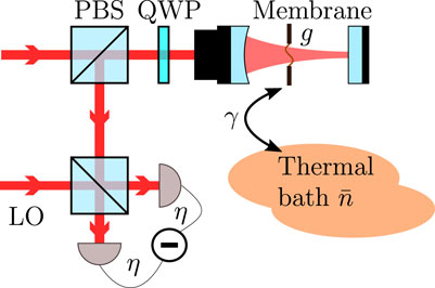
FIGURE 3. Schematic of a micromechanical membrane coupled to a driven cavity with coupling strength g. Before entering the cavity, the linearly polarized driving field is transmitted through a polarizing beam-splitter (PBS) and quarter-wave plate (QWP). After interaction with the cavity and membrane, the outgoing light again passes the QWP, such that it becomes orthogonally polarized to the incoming light. It is reflected off the PBS and superposed on a second beam-splitter with a strong local oscillator (LO) to perform homodyne or heterodyne detection with detection efficiency η. The membrane is additionally coupled to a thermal bath with rate γ and mean phonon number $\bar{n}$.

The adiabatic limit of the conditional optomechanical master equation has been treated in great detail in Hofer and Hammerer (2015). We summarize here the main aspects and then apply it to discuss pre- and retrodiction.

5.1 Optomechanical setup

We consider a mechanical mode with frequency Ω_m coupled to a cavity with resonance frequency ω_c, driven by a strong coherent field with frequency ω₀. We move to a rotating frame with respect to the drive ω₀ and assume the generated intracavity amplitude is large so that we can linearize the radiation pressure interaction. Following standard treatment (Aspelmeyer et al., 2014), this yields

${\widehat{H}}_{\mathrm{l}\mathrm{i}\mathrm{n}}={\widehat{H}}_0+g\left(\widehat{a}+{\widehat{a}}^{†}\right)\left({\widehat{a}}_{\mathrm{c}}+{\widehat{a}}_{\mathrm{c}}^{†}\right),(\mathrm{68a})$

${\widehat{H}}_0={\mathrm{\Omega }}_{\mathrm{m}}{\widehat{a}}^{†}\widehat{a}-{\mathrm{\Delta }}_{\mathrm{c}}{\widehat{a}}_{\mathrm{c}}^{†}{\widehat{a}}_{\mathrm{c}},(\mathrm{68b})$

where ${\widehat{H}}_0$ comprises the local Hamiltonians of cavity and mechanics with Δ_c = ω₀ − ω_c and g ∝ g₀ is the cavity-enhanced optomechanical coupling strength. $\widehat{a}$ and ${\widehat{a}}_{\mathrm{c}}$ are the annihilation operators of the mechanical and cavity mode, respectively.

The cavity field leaks out at a full width at half maximum (FWHM) decay rate κ. The (unconditional) master equation of the joint state ρ_mc of the mechanical and cavity mode reads

$\begin{array}{cc}\hfill {\dot{\rho }}_{\mathrm{m}\mathrm{c}}\left(t\right)& =-i\left[{\widehat{H}}_{\mathrm{l}\mathrm{i}\mathrm{n}},{\rho }_{\mathrm{m}\mathrm{c}}\left(t\right)\right]+\kappa \mathcal{D}[{\widehat{a}}_{\mathrm{c}}]{\rho }_{\mathrm{m}\mathrm{c}}\left(t\right)\hfill \\ \hfill & +{\mathcal{L}}_{\mathrm{t}\mathrm{h}}{\rho }_{\mathrm{m}\mathrm{c}}\left(t\right),\hfill \end{array}(69)$

where we also include a thermal bath,

$\begin{array}{cc}\hfill {\mathcal{L}}_{\mathrm{t}\mathrm{h}}{\rho }_{\mathrm{m}\mathrm{c}}\left(t\right)& =\gamma \left(\bar{n}+1\right)\mathcal{D}[\widehat{a}]{\rho }_{\mathrm{m}\mathrm{c}}\left(t\right)\hfill \\ \hfill & +\gamma \bar{n}\mathcal{D}[{\widehat{a}}^{†}]{\rho }_{\mathrm{m}\mathrm{c}}\left(t\right),\hfill \end{array}(70)$

with mean phonon number $\bar{n}$ which couples with the mechanical oscillator at rate γ (FWHM of the mechanical mode).

We monitor the field that leaks from the cavity using homodyne or heterodyne detection. As usual, the outgoing field is combined on a balanced beam-splitter with a strong local oscillator, and the difference of the measured intensities in the two output beams is the measurement current, depicted at the bottom left of Figure 3. As compared to the conditional master equation Eq. (48) studied in Section 4 on the decaying cavity, we consider here a slightly more general setup where the local oscillator frequency ω_lo may be detuned from the driving frequency ω₀, captured by Δ_lo = ω_lo − ω₀. This realizes a measurement of the outgoing field quadrature operator ${\widehat{a}}_{\text{out}}(t){\mathrm{e}}^{-i{\mathrm{\Delta }}_{\mathrm{l}\mathrm{o}}t+i{\varphi }_{\mathrm{l}\mathrm{o}}}+{\widehat{a}}_{\text{out}}^{†}(t){\mathrm{e}}^{i{\mathrm{\Delta }}_{\mathrm{l}\mathrm{o}}t-i{\varphi }_{\mathrm{l}\mathrm{o}}}$, where ϕ_lo is the tunable phase of the local oscillator. This yields a conditional master equation for cavity and mechanics,

$\begin{array}{cc}\hfill \left(\mathbf{I}\right)\mathrm{d}\rho \left(t\right)& =-i\left[{\widehat{H}}_{\mathrm{l}\mathrm{i}\mathrm{n}},{\rho }_{\mathrm{m}\mathrm{c}}\left(t\right)\right]\mathrm{d}t+\kappa \mathcal{D}[{\widehat{a}}_{\mathrm{c}}]{\rho }_{\mathrm{m}\mathrm{c}}\left(t\right)\mathrm{d}t\hfill \\ \hfill & +{\mathcal{L}}_{\mathrm{t}\mathrm{h}}{\rho }_{\mathrm{m}\mathrm{c}}\left(t\right)\mathrm{d}t\hfill \\ \hfill & +\sqrt{\eta \kappa }\mathcal{H}\left[{\widehat{a}}_{\mathrm{c}}{\mathrm{e}}^{i\left({\mathrm{\Delta }}_{\mathrm{c}}+{\mathrm{\Delta }}_{\mathrm{l}\mathrm{o}}\right)t-i{\varphi }_{\mathrm{l}\mathrm{o}}}\right]\mathrm{d}W\left(t\right),\hfill \end{array}(71)$

where η ∈ [0, 1] is the detection efficiency.

We would like an effective master equation for the mechanics alone. To this end, one can start from the combined master equation Eq. (71) and move to an interaction picture with respect to ${\widehat{H}}_0$. Assuming the cavity field decays rapidly on the time scale established by the optomechanical interaction g/κ ≪ 1, one can adiabatically eliminate the cavity dynamics from the description. For details of this procedure see Hofer and Hammerer (2015) and Hofer and Hammerer (2017). However, before we state the result, we take a closer look at the optomechanical interaction.

5.2 Optomechanical interaction

The linearized radiation-pressure interaction is given by the last term in Eq.68a. The interaction decomposes into two terms: i) a beam-splitter (BS) coupling $g(\widehat{a}{\widehat{a}}_{\mathrm{c}}^{†}+{\widehat{a}}^{†}{\widehat{a}}_{\mathrm{c}})$ and ii) a two-mode squeezing (TMS) part $g(\widehat{a}{\widehat{a}}_{\mathrm{c}}+{\widehat{a}}^{†}{\widehat{a}}_{\mathrm{c}}^{†})$. These give rise to Stokes and anti-Stokes scattering processes (Figure 4). If we work in an interaction picture with respect to ${\widehat{H}}_0$, these terms oscillate at frequencies Ω_m ±Δ_c. For a red-detuned drive, Δ_c = −Ω_m, the BS interaction becomes resonant and is thus enhanced while the TMS interaction oscillates quickly at 2Ω_m and is suppressed. For a blue-detuned drive, Δ_c = Ω_m, the situation is reversed so that the TMS interaction is enhanced and the BS interaction suppressed. For a resonant drive, Δ_c = 0, both processes contribute equally.

FIGURE 4

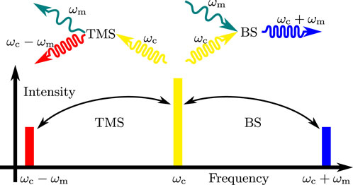
FIGURE 4. Top: Schematic conversion processes occurring in the optomechanical setup depicted in Figure 3 that scatter cavity photons at frequency ω_c into the outgoing sidebands while creating or annihilating a mechanical phonon at frequency Ω_m. Bottom: Spectrum of outgoing light (not to scale). As discussed in Section V B, the linearized optomechanical interaction facilitates two processes: the beam-splitter interaction converts a cavity photon into a phonon and an outgoing photon in the lower (red) sideband at ω_c − Ω_m. Two-mode squeezing combines a cavity photon and a phonon to produce an outgoing photon in the upper (blue) sideband at ω_c + Ω_m.

As we have seen in the initial example in Section 4, the entangling TMS interaction enhances our ability to prepare a conditional mechanical state. Because the outgoing light is entangled with the mechanics, performing a quantum-limited squeezed detection will also project the oscillator onto a squeezed state. On the other hand, the BS interaction generates light with the mechanical state swapped onto it. Observing it allows us to determine what the state was before the interaction but will not enable the preparation of squeezed states. For retrodiction, the situation is reversed. Extracting information about the system in the past from BS light produces squeezed effect operators (sharp measurements) on the past state, while entangled TMS light lets us at best retrodict coherent effect operators. Thus TMS (blue drive) enhances our ability to prepare while the BS interaction (red drive) enhances our ability to retrodict.

5.3 Master equation of the mechanics

In Hofer and Hammerer (2015) and Hofer and Hammerer (2017), the master equation Eq. (71) is turned into an effective evolution equation for the mechanical state ρ_m ≡ ρ through adiabatic elimination of the cavity mode. Since the result is not a proper Lindblad master equation, a rotating wave approximation is needed for which we integrate the dynamics over a short time,

$\left(\mathbf{I}\right)\delta \rho \left(t\right)≔{\int }_t^{t+\delta t}\mathrm{d}\rho \left(\tau \right).(72)$

We are interested here in the case of mechanical oscillators with high quality factors Q = Ω_m/γ, where Ω_m is much larger than other system frequencies set by the optomechanical interaction and decoherence— ${\mathrm{\Omega }}_{\mathrm{m}}\gg g^2/\kappa ,\bar{n}\gamma$. In fact, we assume Ω_m is so much larger that we can choose δt such that ${\mathrm{\Omega }}_{\mathrm{m}}\gg 1/\delta t\gg g^2/\kappa ,\bar{n}\gamma$, which allows us to pull ρ(t) out of all deterministic time integrals since it is approximately constant on this time-scale. Note that this requires $Q\gg \bar{n}$ to be fulfilled with a safe margin. We emphasize that sideband resolution (Ω_m ≫ κ) is not required for the following. We can then perform the rotating wave approximation by dropping all resonant terms oscillating at ± 2Ω_m. Choosing the right phase ϕ_lo and quadrature frame, we find

$\begin{array}{cc}\hfill \left(\mathbf{I}\right)\delta \rho \left(t\right)& ={\mathrm{\Gamma }}_{-}\mathcal{D}\left[\widehat{a}\right]\rho \left(t\right)\delta t+{\mathrm{\Gamma }}_{+}\mathcal{D}\left[{\widehat{a}}^{†}\right]\rho \left(t\right)\delta t\hfill \\ \hfill & +\sqrt{\eta }{\int }_t^{t+\delta t}\mathcal{H}\left[\widehat{C}\left(\tau ;{\mathrm{\Delta }}_{\mathrm{l}\mathrm{o}}\right)\right]\rho \left(\tau \right)\mathrm{d}W\left(\tau \right)\hfill \\ \hfill & +{\mathcal{L}}_{\mathrm{t}\mathrm{h}}\rho \left(t\right)\delta t,\hfill \end{array}(\mathrm{73a})$

with the time-dependent measurement operator

$\begin{array}{cc}\hfill \widehat{C}\left(\tau ;{\mathrm{\Delta }}_{\mathrm{l}\mathrm{o}}\right)& ≔\sqrt{{\mathrm{\Gamma }}_{-}}\widehat{a}{\mathrm{e}}^{-i\left({\mathrm{\Omega }}_{\mathrm{e}\mathrm{f}\mathrm{f}}-{\mathrm{\Delta }}_{\mathrm{l}\mathrm{o}}\right)\tau }\hfill \\ \hfill & +\sqrt{{\mathrm{\Gamma }}_{+}}{\widehat{a}}^{†}{\mathrm{e}}^{i\left({\mathrm{\Omega }}_{\mathrm{e}\mathrm{f}\mathrm{f}}+{\mathrm{\Delta }}_{\mathrm{l}\mathrm{o}}\right)\tau }.\hfill \end{array}(\mathrm{73b})$

The effective mechanical frequency

${\mathrm{\Omega }}_{\mathrm{e}\mathrm{ff}}≔{\mathrm{\Omega }}_{\mathrm{m}}-\sqrt{2}{g}^2\left({\beta }_{+}+{\beta }_{-}\right),(\mathrm{74a})$

${\beta }_{\pm }≔\frac{{\mathrm{\Delta }}_{\mathrm{c}}\pm {\mathrm{\Omega }}_{\mathrm{m}}}{{\left(\kappa /2\right)}^2+{\left({\mathrm{\Delta }}_{\mathrm{c}}\pm {\mathrm{\Omega }}_{\mathrm{m}}\right)}^2}(\mathrm{74b})$

results from a shift of Ω_m due to the optical spring effect, and the rates

${\mathrm{\Gamma }}_{\pm }≔\frac{g^2\kappa }{{\left(\kappa /2\right)}^2+{\left(-{\mathrm{\Delta }}_{\mathrm{c}}\pm {\mathrm{\Omega }}_{\mathrm{m}}\right)}^2}(75)$

are the usual Stokes and anti-Stokes rates known from sideband cooling. From these, we can define two effective cooperativities

$C_{\pm }≔{\mathrm{\Gamma }}_{\pm }/\gamma =C_{\mathrm{c}\mathrm{l}}\frac{{\kappa }^2}{{\kappa }^2+4{\left(-{\mathrm{\Delta }}_{\mathrm{c}}\pm {\mathrm{\Omega }}_{\mathrm{m}}\right)}^2},(76)$

in terms of the classical cooperativity

$C_{\mathrm{c}\mathrm{l}}=\frac{4g^2}{\kappa \gamma }.(77)$

Each C_± compares the rate of the respective (anti-)Stokes process to the incoherent coupling rate of the thermal bath. In the regime κ ≫Ω_m of a broad cavity (Authors Anonymous, 2023c) and assuming κ ≫Δ_c, the cooperativities reduce to the classical cooperativity, C_± ≈ C_cl. As an example of the orders of magnitude involved here, consider Rossi et al. (2018), who realized C ≈ C_cl ∼ 10⁷ and for $\bar{n}\sim 10^5$ a corresponding quantum cooperativity (Aspelmeyer et al., 2014)

$C_q≔\frac{C}{\bar{n}+1}\sim 10^2.(78)$

To obtain a proper master equation from Eq. 73a, we must still perform the integral over the measurement term, which depends on the choice of Δ_lo. However, Eq. 73a already illustrates the point we made in Section 5 B: detuning the driving field affects the optomechanical interaction. Driving on resonance Δ_c = 0, TMS and BS interaction occur with equal strength, reflected by Γ₊ = Γ₋. A blue drive, Δ_c = Ω_m, enhances TMS and causes Γ₊ > Γ₋, while a red drive, Δ_c = −Ω_m, enhances the BS interaction and causes Γ₋ > Γ₊. Additionally, we can tune the local oscillator either to resonantly detect at the driving frequency Δ_lo = 0 or to either the blue or red sideband Δ_lo = ±Ω_eff. We will explore these different dynamics step by step, starting with a resonant drive and resonant detection in the following section, then considering detection of the sidebands in Section 5 E, and finally treating an off-resonant drive with sideband detection in Section 5 F.

5.4 Drive and detect on resonance

We start by exploring a cavity driven on resonance, Δ_c = 0, so we find equal rates Γ₊ = Γ₋≕Γ and equal cooperativities C≔C₊ = C₋ with

$C=C_{\mathrm{c}\mathrm{l}}\frac{{\kappa }^2}{{\kappa }^2+4{\mathrm{\Omega }}_{\mathrm{m}}^2},(79)$

and Ω_eff = Ω_m. The first detection scheme we consider is homodyne detection on resonance, Δ_lo = 0. Plugging this into Eq. 73a yields the measurement operator

$\widehat{C}\left(\tau ;{\mathrm{\Delta }}_{\mathrm{l}\mathrm{o}}=0\right)≔\sqrt{\mathrm{\Gamma }}\left(\widehat{a}{\mathrm{e}}^{-i{\mathrm{\Omega }}_{\mathrm{m}}\tau }+{\widehat{a}}^{†}{\mathrm{e}}^{i{\mathrm{\Omega }}_{\mathrm{m}}\tau }\right),(80)$

$=\sqrt{2\mathrm{\Gamma }}\left(\widehat{x}\cos \left({\mathrm{\Omega }}_{\mathrm{m}}\tau \right)+\widehat{p}\sin \left({\mathrm{\Omega }}_{\mathrm{m}}\tau \right)\right),(81)$

with $\widehat{x}=(\widehat{a}+{\widehat{a}}^{†})/\sqrt{2}$ and $\widehat{p}=-i(\widehat{a}-{\widehat{a}}^{†})/\sqrt{2}$. Using that again, we can extract ρ(t) from the integrals to find the master equation

$\begin{array}{cc}\hfill \left(\mathbf{I}\right)\delta \rho \left(t\right)& ={\mathcal{L}}_{\mathrm{t}\mathrm{h}}\rho \left(t\right)+\mathrm{\Gamma }\mathcal{D}\left[\widehat{a}\right]\rho \left(t\right)\delta t+\mathrm{\Gamma }\mathcal{D}\left[{\widehat{a}}^{†}\right]\rho \left(t\right)\delta t\hfill \\ \hfill & +\sqrt{\eta \mathrm{\Gamma }}\mathcal{H}\left[\widehat{x}\right]\rho \left(t\right)\delta W_{\mathrm{c}}\left(t\right)\hfill \\ \hfill & +\sqrt{\eta \mathrm{\Gamma }}\mathcal{H}\left[\widehat{p}\right]\rho \left(t\right)\delta W_{\mathrm{s}}\left(t\right)\hfill \end{array}(82)$

with the coarse-grained Wiener increments

$\left(\mathbf{I}\right)\delta W_{\mathrm{c}}\left(t\right)≔\sqrt{2}{\int }_t^{t+\delta t}\cos \left({\mathrm{\Omega }}_{\mathrm{m}}\tau \right)\mathrm{d}W\left(\tau \right),(\mathrm{83a})$

$\left(\mathbf{I}\right)\delta W_{\mathrm{s}}\left(t\right)≔\sqrt{2}{\int }_t^{t+\delta t}\sin \left({\mathrm{\Omega }}_{\mathrm{m}}\tau \right)\mathrm{d}W\left(\tau \right).(\mathrm{83b})$

It turns out that these are approximately normalized, $\delta W_{\mathrm{c}}^2(t)=\delta t(1+\mathcal{O}{({\mathrm{\Omega }}_{\mathrm{m}}\delta t)}^{-1})$ and $\delta W_{\mathrm{s}}^2(t)=\delta t(1+\mathcal{O}{({\mathrm{\Omega }}_{\mathrm{m}}\delta t)}^{-1})$, and independent $\delta W_{\mathrm{c}}(t)\delta W_{\mathrm{s}}(t)=\delta t\mathcal{O}{({\mathrm{\Omega }}_{\mathrm{m}}\delta t)}^{-1}$. Thus, we can replace δt → dt, δρ → dρ, and δW_c/s → dW_c/s to obtain effective system dynamics

$\begin{array}{cc}\hfill \left(\mathbf{I}\right)\mathrm{d}\rho \left(t\right)& ={\mathcal{L}}_{\mathrm{t}\mathrm{h}}\rho \left(t\right)+\mathrm{\Gamma }\mathcal{D}\left[\widehat{x}\right]\rho \left(t\right)\mathrm{d}t+\mathrm{\Gamma }\mathcal{D}\left[\widehat{p}\right]\rho \left(t\right)\mathrm{d}t\hfill \\ \hfill & +\sqrt{\eta \mathrm{\Gamma }}\mathcal{H}\left[\widehat{x}\right]\mathrm{d}{W}_{\mathrm{c}}\left(t\right)+\sqrt{\eta \mathrm{\Gamma }}\mathcal{H}\left[\widehat{p}\right]\mathrm{d}{W}_{\mathrm{s}}\left(t\right)\hfill \end{array}(84)$

with independent Wiener increments dW_c(t) and dW_s(t).

5.4.1 Conditional state evolution

Using the notation of Section 2 B, we find $H={\mathbb{0}}_2$, $\mathrm{\Delta }=(\mathrm{\Gamma }+\frac{1}{2}\gamma (2\bar{n}+1)){\mathbb{1}}_2$, and $\mathrm{\Omega }=\frac{1}{2}\gamma \sigma$, as well as the measurement matrices $A=\sqrt{\eta \mathrm{\Gamma }}{\mathbb{1}}_2$, and $B={\mathbb{0}}_2$. As before, we solve ${\dot{V}}_{\rho }=0$ to obtain the steady state covariance $V_{xp}^{\rho }=0$ and equal variances

$\begin{array}{cc}\hfill V_{\rho }^{\infty }& ≔V_{xx}^{\rho }=V_{pp}^{\rho }\hfill \\ \hfill & =\frac{1}{4\eta C}\left(\sqrt{1+8\eta C\left(2C+2\bar{n}+1\right)}-1\right)\hfill \end{array}(85)$

in terms of the cooperativity Eq. 79. The purity is simply the inverse of the variance, $\mathcal{P}(\rho )=1/V_{\rho }^{\infty }$, so it suffices to consider $V_{\rho }^{\infty }$. Note that, as η → 0, the variance approaches its thermal state value $V_{\rho }^{\infty }\to 2\bar{n}+1+2C$. We can compute from the covariance matrix the conditioned drift matrix from Eq. 19 which turns out to be diagonal,

$M_{\rho }^{\infty }={\lambda }_{\rho }{\mathbb{1}}_2,{\lambda }_{\rho }=-\frac{\gamma }{2}\sqrt{1+8\eta C\left(2C+2\bar{n}+1\right)}.(86)$

The degenerate eigenvalue λ_ρ is always real and is negative so long as γ or ηΓ are non-zero and thus guarantee stable dynamics. We obtain the mode functions with which the cosine and sine components of the measurement current are Itô-integrated in Eq. 23 by evaluating the kernel

$\left[\begin{array}{cc}\hfill f_{xc}\left(t\right)\hfill & \hfill f_{xs}\left(t\right)\hfill \\ \hfill f_{pc}\left(t\right)\hfill & \hfill f_{ps}\left(t\right)\hfill \end{array}\right]={\mathrm{e}}^{M_{\rho }^{\infty }t}\left(V_{\rho }^{\infty }{A}^{\mathrm{T}}-\sigma B^{\mathrm{T}}\right).(87)$

We find that f_xs(t) = f_pc(t) = 0 and

$f_{\rho }\left(t\right)≔f_{xc}\left(t\right)=f_{ps}\left(t\right)=\sqrt{\eta \mathrm{\Gamma }}{V}_{\rho }^{\infty }{\mathrm{e}}^{-{\lambda }_{\rho }t},(88)$

which shows that the cosine and sine components of the photocurrent each only enter the corresponding ($\widehat{x}$ or $\widehat{p}$) quadrature.

In the following we assume that ηC ≫ 1 and $\bar{n}\gg 1$ so $\bar{n}+1\approx \bar{n}$. In terms of the quantum cooperativity (Aspelmeyer et al., 2014)

$C_q=\frac{C}{\bar{n}+1}\approx \frac{C}{\bar{n}},(89)$

we find the variance

$V_{\rho }^{\infty }\approx \sqrt{\frac{C_q+1}{\eta C_q}}=\frac{1}{\sqrt{\eta }}\sqrt{1+\frac{1}{C_q}},(90)$

plotted in Figure 5A, and the mode function damping rate is given by

${\lambda }_{\rho }\approx -2\eta \mathrm{\Gamma }\sqrt{\frac{C_q+1}{\eta C_q}}.(91)$

FIGURE 5

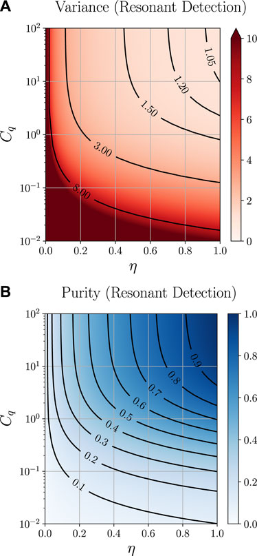
FIGURE 5. (A) Log-linear plot of the steady state variance $V_{\rho }^{\infty }$ (same for $\widehat{x}$ and $\widehat{p}$) from Eq. 85 obtained for homodyne detection on resonance, plotted against detection efficiency η and quantum cooperativity $C_q=C/(\bar{n}+1)$. We chose a bath occupation of $\bar{n}\sim 10^5$ (Rossi et al., 2018), which entails a classical cooperativity of C ∼ 10³…10⁷ in the plotted regime. The exact variance is virtually indistinguishable from its approximate value Eq. 90 because the difference goes as $\sim 1/C$. The plot is also indistinguishable from the exact and approximate variances $V_E^{\infty }$ of the effect operator in Eqs 92 and 93. (B) The purity of the covariance matrix corresponds to the variance in (A).

The equal variances in Eq. 85 and vanishing covariance indicate that we prepare a thermal steady state, which approaches a pure coherent state as η → 1 and C_q → ∞, as we see from the limiting expression Eq. 90 and also from the purity plot in Figure 5B. The exponent λ_ρ in Eqs 86 and (91) determines how fast the mode functions in Eq. 88 decay, and thereby the “memory time” of the conditional state. In the regime where $C_q\gg 1\iff \mathrm{\Gamma }\gg \gamma (\bar{n}+1)$, we find ${\lambda }_{\rho }\approx -2\sqrt{\eta }\mathrm{\Gamma }$, so the mode function is only determined by the measurement rate. If Γ is much larger than typical evolution time scales, it becomes sharply peaked at t, so the conditional state essentially follows the measurement current in real time. However, Γ must stay well below Ω_m or it will violate the assumptions underlying our coarse-graining. In the opposite regime of $C_q\ll 1\iff \mathrm{\Gamma }\ll \gamma (\bar{n}+1)$, the exponent is given by ${\lambda }_{\rho }\approx -2\sqrt{\mathrm{\Gamma }\gamma (\bar{n}+1)/2}$. As Γ → 0, the mode function becomes essentially flat but also goes to zero itself. In this limit, the detection will yield mostly noise and only little signal, so the evolution becomes effectively unconditional.

5.4.2 Retrodiction of POVM elements

We obtain the asymptotic effect operator by solving the Riccati equation resulting from Eq. 43. Again $V_{xp}^E=0$ and

$\begin{array}{ll}\hfill V_E^{\infty }& ≔V_{xx}^E=V_{pp}^E\hfill \\ \hfill & =\frac{1}{4\eta C}\left(\sqrt{1+8\eta C\left(2C+2\bar{n}+1\right)}+1\right),\hfill \end{array}(92)$

$\approx \sqrt{\frac{C_q+1}{\eta C_q}},(93)$

so we find effect operators with equal variance, which corresponds to a POVM realizing a heterodyne measurement.

The asymptotic variance of the retrodicted effect operator is strictly greater than the asymptotic variance of the conditional state $V_E^{\infty }-V_{\rho }^{\infty }=1/(2\eta C)$. The difference vanishes as C → ∞, so the limits in Eqs 90 and(93) are the same, and the plot in Figure 5A also holds for $V_E^{\infty }$. As expected, the exact $V_E^{\infty }$ in Eq. 92 diverges without observations: $V_E^{\infty }\sim 1/(2\eta C)$ as η → 0. Otherwise, the forward and backward dynamics are very similar: we find the same drift matrix as in Eq. 86 with a degenerate negative eigenvalue λ_E = λ_ρ, and the mode function takes the same form as before,

$f_E\left(t\right)=\sqrt{\eta \mathrm{\Gamma }}{V}_E^{\infty }{\mathrm{e}}^{-{\lambda }_{E}t},(94)$

with the strictly greater variance $V_E^{\infty }$ placing more weight on the backward optical mode compared to the evolution of the conditional state. Assuming $C,\bar{n}\gg 1$, forward and backward mode functions become identical.

For both preparation and retrodiction, we see that we can never measure or prepare states with sub-shot noise resolution. In fact, in the ideal limit of perfect detection η → 1 and large cooperativity C_q → ∞, both $V_{\rho }^{\infty }$ and $V_E^{\infty }$ approach 1, so we can at best measure and prepare coherent states. This symmetry is not surprising since detection on resonance means both TMS and BS interaction contribute equally to the observed light. The situation is different when the local oscillator is resonant with either of the sidebands.

5.5 Drive on resonance, detect sidebands

We now detune the local oscillator with respect to the driving laser Δ_lo = ±Ω_m to resolve the information contained in the sidebands located at ω_c ±Ω_m. Recalling the general equation Eq. (73), we see that detecting the red sideband Δ_lo = −Ω_m makes ${\widehat{a}}^{†}$ resonant while $\widehat{a}$ oscillates at −2Ω_m and yields the measurement operator

$\widehat{C}\left(\tau ;{\mathrm{\Delta }}_{\mathrm{l}\mathrm{o}}=-{\mathrm{\Omega }}_{\mathrm{m}}\right)=\sqrt{\mathrm{\Gamma }}\left(\widehat{a}{\mathrm{e}}^{-2i{\mathrm{\Omega }}_{\mathrm{m}}\tau }+{\widehat{a}}^{†}\right).(95)$

Resonant detection of the blue sideband with Δ_lo = Ω_m analogously makes $\widehat{a}$ resonant and results in

$\widehat{C}\left(\tau ;{\mathrm{\Delta }}_{\mathrm{l}\mathrm{o}}={\mathrm{\Omega }}_{\mathrm{m}}\right)=\sqrt{\mathrm{\Gamma }}\left(\widehat{a}+{\widehat{a}}^{†}{\mathrm{e}}^{2i{\mathrm{\Omega }}_{\mathrm{m}}\tau }\right).(96)$

Thus, we expect after coarse-graining to better observe an effect of the TMS interaction on the red sideband and of the BS interaction on the blue sideband. To evaluate the integrals in Eq. 73a, we introduce

$\left(\mathbf{I}\right)\delta W_0\left(t\right)≔{\int }_t^{t+\delta t}\mathrm{d}W\left(\tau \right),(\mathrm{97a})$

$\left(\mathbf{I}\right)\delta W_{\mathrm{c},2}\left(t\right)≔\sqrt{2}{\int }_t^{t+\delta t}\cos \left(2{\mathrm{\Omega }}_{\mathrm{m}}\tau \right)\mathrm{d}W\left(\tau \right),(\mathrm{97b})$

$\left(\mathbf{I}\right)\delta W_{\mathrm{s},2}\left(t\right)≔\sqrt{2}{\int }_t^{t+\delta t}\sin \left(2{\mathrm{\Omega }}_{\mathrm{m}}\tau \right)\mathrm{d}W\left(\tau \right),(\mathrm{97c})$

analogous to Eq. 83a, which separates the photocurrent oscillating at twice the mechanical frequency from its DC component (at the given sideband frequency). As before, these are approximately normalized and independent of one another (up to $\mathcal{O}{({\mathrm{\Omega }}_{\mathrm{m}}\delta t)}^{-1}$), so we treat them as independent Wiener increments. Making the replacements δt → dt and δW_α → dW_α, we obtain two coarse-grained master equations depending on the choice of Δ_lo = ±Ω_m.

5.5.1 Detecting the red sideband

We first consider the local oscillator tuned to the red sideband Δ_lo = −Ω_m. This yields the coarse-grained master equation

$\begin{array}{cc}\hfill \left(\mathbf{I}\right)\mathrm{d}\rho \left(t\right)& ={\mathcal{L}}_{\mathrm{t}\mathrm{h}}\rho \left(t\right)+\mathrm{\Gamma }\mathcal{D}\left[\widehat{x}\right]\rho \left(t\right)\mathrm{d}t+\mathrm{\Gamma }\mathcal{D}\left[\widehat{p}\right]\rho \left(t\right)\mathrm{d}t\hfill \\ \hfill & +\sqrt{\eta \mathrm{\Gamma }}\mathcal{H}\left[\widehat{a}\right]\rho \left(t\right)\mathrm{d}{W}_{\mathrm{c},2}\left(t\right)\hfill \\ \hfill & -\sqrt{\eta \mathrm{\Gamma }}\mathcal{H}\left[i\widehat{a}\right]\rho \left(t\right)\mathrm{d}{W}_{\mathrm{s},2}\left(t\right)\hfill \\ \hfill & +\sqrt{\eta \mathrm{\Gamma }}\mathcal{H}\left[{\widehat{a}}^{†}\right]\rho \left(t\right)\mathrm{d}{W}_0\left(t\right).\hfill \end{array}(98)$

Analogous to the case of resonant detection, we can use the Gaussian formalism to compute the conditional steady state variances,

$V_{xx}^{\rho }=\frac{1}{3\eta C}\left(\sqrt{1+4\eta C\left(\left(3-2\eta \right)C+3\bar{n}+2\right)}-1\right)-\frac{1}{3},,(99)$

$V_{pp}^{\rho }=\frac{1}{\eta C}\left(\sqrt{1+4\eta C\left(C+\bar{n}\right)}-1\right)+1,(100)$

which, for $C,\bar{n}\gg 1$, become approximately

$V_{xx}^{\rho }\approx \frac{2}{3}\sqrt{\frac{\left(3-2\eta \right)C_q+3}{\eta C_q}}-\frac{1}{3},(101)$

$V_{pp}^{\rho }\approx 2\sqrt{\frac{C_q+1}{\eta C_q}}+1.(102)$

To find the corresponding Gaussian effect operators realizable through retrodiction, we could translate the full master equation above to an effect equation and then apply the Gaussian formalism as before. Instead, we take the shortcut of directly reading off the Riccati equation Eq. (43) from the corresponding Riccati equation of the conditional state. Solving it yields the asymptotic variances

$V_{xx}^E=\frac{1}{3\eta C}\left(\sqrt{1+4\eta C\left(\left(3-2\eta \right)C+3\bar{n}+2\right)}+1\right)+\frac{1}{3},(103)$

$V_{pp}^E=\frac{1}{\eta C}\left(\sqrt{1+4\eta C\left(C+\bar{n}\right)}+1\right)-1,(104)$

which for $C,\bar{n}\gg 1$ approach

$V_{xx}^E\approx \frac{2}{3}\sqrt{\frac{\left(3-2\eta \right)C_q+3}{\eta C_q}}+\frac{1}{3},(105)$

$V_{pp}^E\approx 2\sqrt{\frac{C_q+1}{\eta C_q}}-1.(106)$

Considering the ideal limit η → 1 and C_q → ∞, we find

$V_{xx}^E\to 1,V_{pp}^E\to 1(107)$

for the effect operator, so at best we retrodict POVMs that project onto coherent states. On the other hand, we find

$V_{xx}^{\rho }\to \frac{1}{3},V_{pp}^{\rho }\to 3(108)$

for the conditional steady state, showing that we can, in principle, prepare squeezed states. Necessary conditions for going below shot noise in the preparation are C_q > 1 and η > 1/2 since

$V_{xx}^{\rho }<1\iff \eta >\frac{C+\bar{n}}{2C}\approx \frac{1}{2}\left(1+\frac{1}{C_q}\right),(109)$

which is confirmed by the plot of $V_{xx}^{\rho }$ in Figure 6A. However, even with one quadrature below shot noise, the prepared state will never be entirely pure (Figure 6B).

FIGURE 6

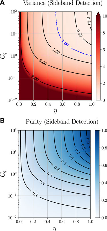
FIGURE 6. (A) Linear-logarithmic plot of the approximate steady state variances $V_{xx}^{\rho }$ and $V_{xx}^E$ from Eqs 101 and 118 plotted against detection efficiency η and quantum cooperativity C_q in the limit of large cooperativity C ≫ 1. The dashed line denotes the shot noise-limited variance of the vacuum state at V_xx = 1. (B) The purity of the covariance matrices corresponds to the variances plotted in (A).

5.5.2 Detecting the blue sideband

Tuning the local oscillator to the blue sideband, we find for Δ_lo = +Ω_m the master equation

$\begin{array}{cc}\hfill \left(\mathbf{I}\right)\mathrm{d}\rho \left(t\right)& ={\mathcal{L}}_{\mathrm{t}\mathrm{h}}\rho \left(t\right)+\mathrm{\Gamma }\mathcal{D}\left[\widehat{x}\right]\rho \left(t\right)\mathrm{d}t+\mathrm{\Gamma }\mathcal{D}\left[\widehat{p}\right]\rho \left(t\right)\mathrm{d}t\hfill \\ \hfill & +\sqrt{\eta \mathrm{\Gamma }}\mathcal{H}\left[{\widehat{a}}^{†}\right]\rho \left(t\right)\mathrm{d}{W}_{\mathrm{c},2}\left(t\right)\hfill \\ \hfill & +\sqrt{\eta \mathrm{\Gamma }}\mathcal{H}\left[i{\widehat{a}}^{†}\right]\rho \left(t\right)\mathrm{d}{W}_{\mathrm{s},2}\left(t\right)\hfill \\ \hfill & +\sqrt{\eta \mathrm{\Gamma }}\mathcal{H}\left[\widehat{a}\right]\rho \left(t\right)\mathrm{d}{W}_0\left(t\right),\hfill \end{array}(110)$

which asymptotically results in a conditional state with variances

$V_{xx}^{\rho }=\frac{1}{3\eta C}\left(\sqrt{1+4\eta C\left(\left(3-2\eta \right)C+3\bar{n}+1\right)}-1\right)+\frac{1}{3},(111)$

$V_{pp}^{\rho }=\frac{1}{\eta C}\left(\sqrt{1+4\eta C\left(C+\bar{n}+1\right)}-1\right)-1,(112)$

which for $C,\bar{n}\gg 1$ become approximately

$V_{xx}^{\rho }\approx \frac{1}{3}\sqrt{\frac{\left(3-2\eta \right)C_q+3}{\eta C_q}}+\frac{1}{6},(113)$

$V_{pp}^{\rho }\approx \sqrt{\frac{C_q+1}{\eta C_q}}-\frac{1}{2}.(114)$

We see here that, in the limit of η → 1 and C_q → ∞, the variances approach

$\begin{array}{llll}\hfill V_{xx}^{\rho }& \to 1,\hfill & \hfill V_{pp}^{\rho }& \to 1,\hfill \end{array}(115)$

so we can at best prepare coherent states.

To find the corresponding effect operators, we again translate the forward Riccati equation directly to a corresponding backward equation. This yields the asymptotic variances

$V_{xx}^E=\frac{1}{3\eta C}\left(\sqrt{1+4\eta C\left(\left(3-2\eta \right)C+3\bar{n}+1\right)}+1\right)-\frac{1}{3},(116)$

$V_{pp}^E=\frac{1}{\eta C}\left(\sqrt{1+4\eta C\left(C+\bar{n}+1\right)}+1\right)+1,(117)$

which for $C,\bar{n}\gg 1$ become approximately

$V_{xx}^E\approx \frac{2}{3}\sqrt{\frac{\left(3-2\eta \right)C_q+3}{\eta C_q}}-\frac{1}{3},(118)$

$V_{pp}^E\approx 2\sqrt{\frac{C_q+1}{\eta C_q}}+1.(119)$

Considering the ideal limit η → 1 and C_q → ∞, we see that the asymptotic effect operators can in principle project onto squeezed states

$V_{xx}^E\to \frac{1}{3},V_{pp}^E\to 3,(120)$

provided C_q > 1 and η > 1/2 since

$V_{xx}^E<1\iff \eta >\frac{C+\bar{n}+1}{2C}=\frac{1}{2}\left(1+\frac{1}{C_q}\right).(121)$

Since both the limiting $\widehat{x}$-variances Eqs 101 and (118) and corresponding $\widehat{p}$-variances agree, the plots in Figure 6 also hold for the effect operators retrodicted on the blue sideband.

These results are summarized in Table 2: for large quantum cooperativity and resonant drive, homodyne detection of the blue (red) sideband generates coherent (squeezed) conditional states and squeezed (coherent) retrodictive POVMs. This conforms with the expectation that blue (red) sideband photons have been generated via a beam-splitter (two-mode squeezing) interaction, as discussed in Section 5 B. Thus, these two cases perform qualitatively similarly to the basic examples studied in Section 4 and Table I. There is, of course, a significant quantitative difference as, for example, the squeezed POVM realized by resonant drive exhibits a noise reduction by 66% only. A perfect quadrature measurement, such as found in Section 4, would require infinite squeezing. In order to achieve this, the driving field has to be detuned from cavity resonance, as will be discussed next.

TABLE 2

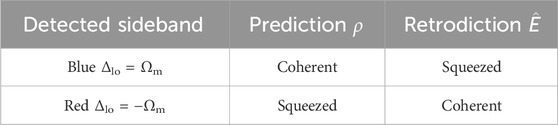
TABLE 2. Conditional states and retrodictive POVMs generated by resonant drive and homodyne detection of the blue or red sideband.

5.6 Off-resonant drive

The case of an off-resonant drive, Δ_c ≠ 0, is also very relevant in experiments—for example, performing sideband cooling or preparing squeezed mechanical states in pulsed schemes (Hofer and Hammerer, 2017). Detuning also enables richer retrodictive dynamics since it allows selective enhancement and suppression of the Stokes and anti-Stokes rates Γ_± and, thus, the BS and TMS components of the optomechanical interaction. Of course, it must be remembered that a detuned drive requires more power to maintain the same level of linear coupling.

To analyze the effects of non-zero detuning, we need to return to the original coarse-grained master equation Eq. (73). Evaluating the integral over the measurement term for homodyne detection of the carrier or sideband frequencies proceeds analogously to the previous sections. We only need to remember that the sidebands are now located at ω_c ±Ω_eff with the effective frequency Ω_eff from Eq. 74a. The Stokes and anti-Stokes rates Γ_± from Eq. 75 are no longer equal to a single rate

$\mathrm{\Gamma }=\frac{g^2\kappa }{{\left(\kappa /2\right)}^2+{\mathrm{\Omega }}_{\mathrm{m}}^2},(122)$

but can be written as

${\mathrm{\Gamma }}_{\pm }=\mathrm{\Gamma }{f}_{\pm },(\mathrm{123a})$

$f_{\pm }≔\frac{1+4{\left({\mathrm{\Omega }}_{\mathrm{m}}/\kappa \right)}^2}{1+4{\left(-{\mathrm{\Delta }}_{\mathrm{c}}\pm {\mathrm{\Omega }}_{\mathrm{m}}\right)}^2/{\kappa }^2}.(\mathrm{123b})$

For a blue-detuned drive, Δ_c > 0 such that Γ₊ ≥Γ₋ + γ, the mechanical dynamics are unstable. Since we are interested in stationary states obtained through continuous driving and observation, we will thus consider only a red-detuned drive, Δ_c < 0, in the following. We see that with Δ_c = −Ω_m, we can enhance Γ₋ by a factor $f_{-}=1+4{({\mathrm{\Omega }}_{\mathrm{m}}/\kappa )}^2>1$ while suppressing Γ₊ by $f_{+}=(1+4{({\mathrm{\Omega }}_{\mathrm{m}}/\kappa )}^2)/(1+16{({\mathrm{\Omega }}_{\mathrm{m}}/\kappa )}^2)<1$. In the broad cavity regime (Ω_m/κ ≪ 1), this imbalance becomes negligible, so we do not expect any benefit from a detuned drive, but, whenever Ω_m/κ > 1, the enhancement of Γ₋ greatly enhances our ability to retrodict POVMs with sub-shot noise resolution, as will now be shown.

Analogous to the previous sections, we solve the Riccati equations for the asymptotic covariance matrices of filtered Gaussian states and retrodicted POVM elements. We will only consider $\widehat{x}$ variances, since the results can be applied to any other quadrature by changing the local oscillator phase. Additionally, since we are interested in fundamental limits, we consider only detection of the sidebands that are optimal for preparation and retrodiction, respectively, in the sense that they minimize the stationary variance: the red sideband Δ_lo = −Ω_eff for preparation and the blue sideband Δ_lo = Ω_eff for retrodiction. The solutions are conveniently expressed in terms of the classical and quantum cooperativities

$C_{\pm }≔\frac{{\mathrm{\Gamma }}_{\pm }}{\gamma }=C{f}_{\pm },(124)$

$C_q^{\pm }≔\frac{C_{\pm }}{\bar{n}+1}=C_q{f}_{\pm },(125)$

where the “bare” cooperativities C and C_q are the same as for a resonant drive considered in the previous sections. The solution for a conditional Gaussian steady state prepared by observing the red sideband Δ_lo = −Ω_eff then reads

$\begin{array}{l}\hfill \begin{array}{cccc}\hfill V_{xx}^{\rho }& =\frac{1}{\eta \left(C_{-}+2C_{+}\right)}\left(-1-\left(1-\eta \right)C_{-}\right.\hfill & \hfill & +\left.\left(1-2\eta \right)C_{+}+\sqrt{r}\right),\hfill \end{array}\end{array}(\mathrm{126a})$

$\begin{array}{l}\hfill \begin{array}{cc}\hfill r& ≔{\left(C_{-}-C_{+}+1\right)}^2+4\eta \left(3-2\eta \right)C_{-}{C}_{+}\hfill \\ \hfill & +8\eta C_{+}\left(\bar{n}+1\right)+4\bar{n}\eta C_{-}.\hfill \end{array}\end{array}(\mathrm{126b})$

Here, we see in the broad cavity regime Ω_m/κ ≪ 1, where C₋ ≈ C₊ ≈ C, that the variance is just given by what one finds by driving on resonance. Thus, the minimal variance obtained for η = 1 and C_q → ∞ will be given by $V_{xx}^{\rho }\to 1/3<1$ and thus corresponds to a squeezed state. On the other hand, when Ω_m/κ > 1, we find that $C_q^{-}\gg C_q^{+}$ and $V_{xx}^{\rho }\to 1$, so we can at best prepare coherent states. The effect of different cavity linewidths is also depicted in Figure 7, where we see that a red-detuned drive does not help preparation as expected.

FIGURE 7

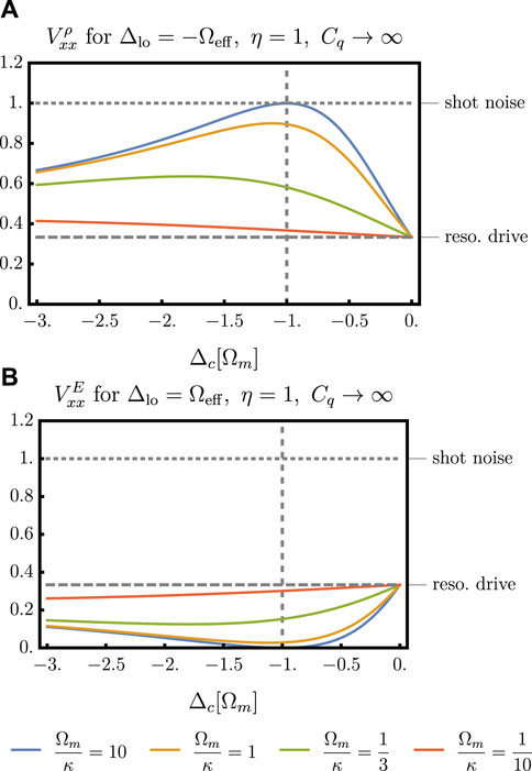
FIGURE 7. (A) Conditional steady state variance $V_{xx}^{\rho }$ from Eq. V F and (B) asymptotic variance $V_{xx}^E$ of retrodicted effect operators from Eq. 127a in the ideal limit of η = 1 and C_q → ∞ plotted against detuning of the drive Δ_c in units of the mechanical frequency Ω_m. Different curves correspond to different values of Ω_m/κ ranging from the broad cavity (Ω_m/κ ≪ 1) to the sideband-resolved regime (Ω_m/κ ≫ 1). The upper dotted line is the shot noise limit $V_{xx}^{\rho }=V_{xx}^E=1$ and the lower dashed line the limit obtainable with a resonant drive ($V_{xx}^{\rho }=V_{xx}^E=1/3$).

We can compare these results to the asymptotic variance of a Gaussian effect operator retrodicted by observing the blue sideband, Δ_lo = Ω_eff, which reads

$\begin{array}{l}\hfill \begin{array}{cccc}\hfill V_{xx}^E& =\frac{1}{\eta \left(2C_{-}+C_{+}\right)}\left(1-\left(1-\eta \right)C_{+}\right.\hfill & \hfill & +\left.\left(1-2\eta \right)C_{-}+\sqrt{s}\right),\hfill \end{array}\end{array}(\mathrm{127a})$

$\begin{array}{l}\hfill \begin{array}{cc}\hfill s& ≔{\left(C_{-}-C_{+}+1\right)}^2+4\eta \left(3-2\eta \right)C_{-}{C}_{+}\hfill \\ \hfill & +4\eta C_{+}\left(\bar{n}+1\right)+8\bar{n}\eta C_{-}.\hfill \end{array}\end{array}(\mathrm{127b})$

Here, we find that, to retrodict POVMs with sub-shot noise resolution $V_{xx}^E<1$, the detection efficiency must satisfy

$\eta >\frac{1}{2}\left(1+\frac{1}{C_q^{-}}\right),(128)$

and thus necessarily η > 1/2 but also $C_q^{-}>1$. This is interesting because it means that, with detuning Δ_c = −Ω_m, we no longer require a large “bare” cooperativity C_q > 1 to measure with sub-shot noise resolution but only a large product $C_q(1+4{({\mathrm{\Omega }}_{\mathrm{m}}/\kappa )}^2)>1$, which can be rewritten as

${\left(\frac{{\mathrm{\Omega }}_{\mathrm{m}}}{\kappa }\right)}^2>\frac{1-C_q}{4C_q}.(129)$

Thus, a detuned drive in the sideband-resolved regime allows retrodiction of POVMs that beat the shot noise limit even for sub-unit quantum cooperativities. In fact, whenever Ω_m/κ ≫ 1 such that $C_q^{-}\gg 1$ and $C_q^{-}\gg C_q^{+}$, the minimal variance will approach

$V_{xx}^E\to \frac{1-\eta }{\eta },(130)$

as can also be seen in Figure 8, where we plot the achievable variances for conservative values of C_q = 1/2 and η = 0.77. These results show that, with an off-resonant (red-detuned) drive and using only continuous measurements, measurement is possible with sub-shot noise variance limited only by the detection efficiency η.

FIGURE 8

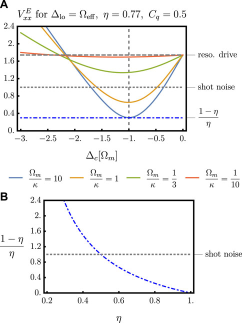
FIGURE 8. (A) The asymptotic variance $V_{xx}^E$ of retrodicted effect operators from Eq. 127a plotted against detuning of the drive Δ_c in units of the mechanical frequency Ω_m. Instead of the ideal limit η = 1 and C_q → ∞ used to create Figure 7, (B) we consider a realistic efficiency η = 0.77 and sub-unit cooperativity C_q = 1/2. As the cavity enters the sideband-resolved regime where Ω_m/κ > 1, the variance approaches $V_{xx}^E\to (1-\eta )/\eta$ (dash-dotted line). (B) This limiting value of the variance is plotted in the bottom figure against η.

In summary, it is possible to perform quadrature measurements of the mechanical state with sub-shot noise variance through continuous monitoring of the cavity output. By using a red-detuned cavity drive and sufficiently efficient homodyne detection of the blue sideband of the output, one achieves a squeezed retrodictive POVM realizing a quadrature measurement for the past mechanical state. In the resolved sideband limit, the quality of the quadrature measurement is essentially only limited by the detection efficiency and does not require a quantum cooperativity larger than 1.

6 Conclusion and outlook

We have given here a self-contained introduction to the theory of retrodictive POVMs, demonstrating the potential to retrieve information about the initial quantum state of a system based on the outcomes of a continuous measurement process. The general formalism has been illustrated in detail for linear quantum systems and applied to realistic models of optomechanical systems.

The application of our theoretical framework to optomechanics has revealed promising avenues for achieving retrodictive state analysis. By characterizing achievable retrodictive POVMs in various optomechanical operating modes, such as resonant and off-resonant driving fields, we have illustrated the potential for precise retrodictive measurements of mechanical oscillators. Notably, our findings reveal the possibility of nearly ideal quadrature measurements, offering direct access to the position or momentum distribution of mechanical oscillators at specific time instances. This advance opens doors to novel possibilities in quantum state tomography and of non-Gaussian states, albeit with the caveat of being inherently destructive.

We hope that this presentation will facilitate and advance the use of retrodictive POVMs in other linear quantum systems beyond optomechanics. Extending the formalism to more complex and nonlinear systems presents an intriguing challenge. As quantum technology continues to advance, the insights gained from this work will contribute to the expanding toolkit of quantum state analysis and manipulation.

We thank Klaus Mølmer, Albert Schließer, Stefan Danilishin, Sebastian Hofer, David Reeb, Reinhard Werner, and Lars Dammeier for discussions on this topic. We acknowledge funding by the Deutsche Forschungsgemeinschaft (DFG, German Research Foundation) through Project-ID 274200144–SFB 1227 (projects A06) and Project-ID 390837967–EXC 2123.

Data availability statement

The original contributions presented in the study are included in the article/Supplementary Material; further inquiries can be directed to the corresponding author.

Author contributions

JL: writing–original draft and writing–review and editing. KH: writing–original draft and writing–review and editing.

Funding

The author(s) declare that financial support was received for the research, authorship, and/or publication of this article. This research was funded by Deutsche Forschungsgemeinschaft (DFG, German Research Foundation) through Project-ID 274200144–SFB 1227 (projects A06) and Project-ID 390837967–EXC 2123.

Conflict of interest

The authors declare that the research was conducted in the absence of any commercial or financial relationships that could be construed as a potential conflict of interest.

Publisher’s note

All claims expressed in this article are solely those of the authors and do not necessarily represent those of their affiliated organizations, or those of the publisher, the editors, and the reviewers. Any product that may be evaluated in this article, or claim that may be made by its manufacturer, is not guaranteed or endorsed by the publisher.

Supplementary material

The Supplementary Material for this article can be found online at: https://www.frontiersin.org/articles/10.3389/frqst.2023.1294905/full#supplementary-material

References

Adesso, G., Ragy, S., and Lee, A. R. (2014). Continuous variable quantum information: Gaussian states and beyond. Open Syst. Inf. Dyn. 21, 1440001. doi:10.1142/s1230161214400010

CrossRef Full Text | Google Scholar

Aspelmeyer, M., Kippenberg, T. J., and Marquardt, F. (2014). Cavity optomechanics. Rev. Mod. Phys. 86, 1391–1452. doi:10.1103/revmodphys.86.1391

CrossRef Full Text | Google Scholar

Authors Anonymous (2023a). Hence α = (δI(t)2/δt)1/2with δt chosen as small as possible without violating the assumption that the noise is indeed white, i. e., has independent increments from one moment to the next.

Google Scholar

Authors Anonymous (2023b). Let V = S^T (T⊕T)S be the symplectic diagonalization of the covariance matrix V, that is S is a symplectic matrix with S^TσS = σ and T is a diagonal matrix with entries τ_k. Then Γ = S⁻¹(K⊕K)(S⁻¹)^T where K is a diagonal matrix with entries κ_k such that τ_k = (1 − e^−κ_k)⁻¹.

Google Scholar

Authors Anonymous (2023c). We assumed Ω_m ≫ g²/κ for the rotating wave approximation which imposes Ω_m/κ ≫ (g/κ)². However, we also used g/κ ≪ 1 to eliminate the cavity so (g/κ)² is a small parameter and the derivation holds for a range of linewidths from the sideband-resolved (κ ≪Ω_m) to the broad cavity regime (κ ≫Ω_m).

Google Scholar

Authors Anonymous (2023d). When computing dˆE (t) of the effect operator in [47] it is important to reintroduce the initial time which was set to zero by Wiseman, and to take the derivative with respect to this time.

Google Scholar

Authors Anonymous (2023e). Such terms can always be set to zero by a suitable shift $\widehat{\mathbf{r}}\to \widehat{\mathbf{r}}+\mathit{\xi }$ where $\mathit{\xi }\in {\mathbb{R}}^{2M}$

Google Scholar

Bao, H., Duan, J., Jin, S., Lu, X., Li, P., Qu, W., et al. (2020a). Spin squeezing of 1011 atoms by prediction and retrodiction measurements. Nature 581, 159–163. doi:10.1038/s41586-020-2243-7

PubMed Abstract | CrossRef Full Text | Google Scholar

Bao, H., Jin, S., Duan, J., Jia, S., Mølmer, K., Shen, H., et al. (2020b). Retrodiction beyond the Heisenberg uncertainty relation. Nat. Commun. 11, 5658. doi:10.1038/s41467-020-19495-1

PubMed Abstract | CrossRef Full Text | Google Scholar

Barchielli, A., and Gregoratti, M. (2009). Quantum trajectories and measurements in continuous time, lecture notes in physics. Berlin, Heidelberg: Springer Berlin Heidelberg.

Google Scholar

Barnett, S., and Radmore, P. (1997). Methods in theoretical quantum Optics. Oxford: Oxford University Press.

Google Scholar

Barnett, S. M., Pegg, D. T., and Jeffers, J. (2000). Bayes’ theorem and quantum retrodiction. J. Mod. Opt. 47, 1779–1789. doi:10.1080/09500340008232431

CrossRef Full Text | Google Scholar

Barnett, S. M., Pegg, D. T., Jeffers, J., and Jedrkiewicz, O. (2001). Master equation for retrodiction of quantum communication signals. Phys. Rev. Lett. 86, 2455–2458. doi:10.1103/physrevlett.86.2455

PubMed Abstract | CrossRef Full Text | Google Scholar

Bouten, L., Van Handel, R., and James, M. R. (2007). An introduction to quantum filtering. SIAM J. Control Optim. 46, 2199–2241. doi:10.1137/060651239

CrossRef Full Text | Google Scholar

Chantasri, A., Guevara, I., Laverick, K. T., and Wiseman, H. M. (2021). Unifying theory of quantum state estimation using past and future information. Phys. Rep. 930, 1–40. doi:10.1016/j.physrep.2021.07.003

CrossRef Full Text | Google Scholar

Chen, Y. (2013). Macroscopic quantum mechanics: theory and experimental concepts of optomechanics. J. Phys. B Atomic, Mol. Opt. Phys. 46, 104001. doi:10.1088/0953-4075/46/10/104001

CrossRef Full Text | Google Scholar

Eisert, J., and Wolf, M. M. (2007). “Gaussian quantum channels,” in Quantum information with continuous variables of atoms and light (London, UK: Imperial College Press), 23–42.

CrossRef Full Text | Google Scholar

Fiurášek, J., and Mišta, L. (2007). Gaussian localizable entanglement. Phys. Rev. 75, 060302. doi:10.1103/PhysRevA.75.060302

CrossRef Full Text | Google Scholar

Foroozani, N., Naghiloo, M., Tan, D., Mølmer, K., and Murch, K. W. (2016). Correlations of the time dependent signal and the state of a continuously monitored quantum system. Phys. Rev. Lett. 116, 110401. doi:10.1103/physrevlett.116.110401

PubMed Abstract | CrossRef Full Text | Google Scholar

Gammelmark, S., Julsgaard, B., and Mølmer, K. (2013). Past quantum states of a monitored system. Phys. Rev. Lett. 111, 160401. doi:10.1103/physrevlett.111.160401

PubMed Abstract | CrossRef Full Text | Google Scholar

Gardiner, C. (2009). Stochastic methods: a handbook for the natural and social sciences. Berlin, Germany: Springer-Verlag Berlin Heidelberg.

Google Scholar

Gardiner, C., and Zoller, P. (2010). “Springer series in synergetics,” in Quantum noise: a handbook of markovian and non-markovian quantum stochastic methods with applications to quantum Optics (Berlin, Germany: Springer).

Google Scholar

Genoni, M. G., Lami, L., and Serafini, A. (2016). Conditional and unconditional Gaussian quantum dynamics. Contemp. Phys. 57, 331–349. doi:10.1080/00107514.2015.1125624

CrossRef Full Text | Google Scholar

Geremia, J., Stockton, J. K., Doherty, A. C., and Mabuchi, H. (2003). Quantum kalman filtering and the heisenberg limit in atomic magnetometry. Phys. Rev. Lett. 91, 250801. doi:10.1103/physrevlett.91.250801

PubMed Abstract | CrossRef Full Text | Google Scholar

Giedke, G. (2001). Quantum information and continuous variable systems. Ph.D. thesis. Berlin, Germany: Springer.

Google Scholar

Guevara, I., and Wiseman, H. (2015). Quantum state smoothing. Phys. Rev. Lett. 115, 180407. doi:10.1103/physrevlett.115.180407

PubMed Abstract | CrossRef Full Text | Google Scholar

Hacohen-Gourgy, S., and Martin, L. S. (2020). Continuous measurements for control of superconducting quantum circuits. Adv. Phys. X 5, 1813626. doi:10.1080/23746149.2020.1813626

CrossRef Full Text | Google Scholar

Heinosaari, T., Holevo, A. S., and Wolf, M. M. (2010). The semigroup structure of Gaussian channels. Quantum Inf. Comput. 10, 0619. doi:10.26421/QIC10.7-8-4

CrossRef Full Text | Google Scholar

Hofer, S. G., and Hammerer, K. (2015). Entanglement-enhanced time-continuous quantum control in optomechanics. Phys. Rev. A 91, 033822. doi:10.1103/physreva.91.033822

CrossRef Full Text | Google Scholar

Hofer, S. G., and Hammerer, K. (2017). Quantum control of optomechanical systems. Adv. Atomic, Mol. Opt. Phys. 66, 263–374. doi:10.1016/bs.aamop.2017.03.003

CrossRef Full Text | Google Scholar

Huang, Z., and Sarovar, M. (2018). Smoothing of Gaussian quantum dynamics for force detection. Phys. Rev. A 97, 1712, 042106. doi:10.1103/physreva.97.042106

CrossRef Full Text | Google Scholar

Ivan, J. S., Kumar, M. S., and Simon, R. (2012). A measure of non-Gaussianity for quantum states. Quantum Inf. Process. 11, 853–872. doi:10.1007/s11128-011-0314-2

CrossRef Full Text | Google Scholar

Iwasawa, K., Makino, K., Yonezawa, H., Tsang, M., Davidovic, A., Huntington, E., et al. (2013). Quantum-limited mirror-motion estimation. Phys. Rev. Lett. 111, 163602. doi:10.1103/physrevlett.111.163602

PubMed Abstract | CrossRef Full Text | Google Scholar

Jacobs, K. (2014). Quantum measurement theory and its applications. Cambridge: Cambridge University Press.

Google Scholar

Jacobs, K., and Steck, D. A. (2006). A straightforward introduction to continuous quantum measurement. Contemp. Phys. 47, 279–303. doi:10.1080/00107510601101934

CrossRef Full Text | Google Scholar

Khalili, F., Danilishin, S., Miao, H., Müller-Ebhardt, H., Yang, H., and Chen, Y. (2010). Preparing a mechanical oscillator in non-Gaussian quantum states. Phys. Rev. Lett. 105, 070403. doi:10.1103/physrevlett.105.070403

PubMed Abstract | CrossRef Full Text | Google Scholar

Kohler, J., Gerber, J. A., Deist, E., and Stamper-Kurn, D. M. (2020). Simultaneous retrodiction of multimode optomechanical systems using matched filters. Phys. Rev. A 101, 023804. doi:10.1103/physreva.101.023804

CrossRef Full Text | Google Scholar

Kong, J., Jiménez-Martínez, R., Troullinou, C., Lucivero, V. G., Tóth, G., and Mitchell, M. W. (2020). Measurement-induced, spatially-extended entanglement in a hot, strongly-interacting atomic system. Nat. Commun. 11, 2415. doi:10.1038/s41467-020-15899-1

PubMed Abstract | CrossRef Full Text | Google Scholar

Kuznetsov, D. F. (2017). Multiple ito and Stratonovich stochastic integrals: fourier-legendre and trogonometric expansions. Approx. Formulas, Differ. Equations Control Process. 1.

Google Scholar

Liao, J., Jost, M., Schaffner, M., Magno, M., Korb, M., Benini, L., et al. (2019). FPGA implementation of a Kalman-based motion estimator for levitated nanoparticles. IEEE Trans. Instrum. Meas. 68, 2374–2386. doi:10.1109/tim.2018.2879146

CrossRef Full Text | Google Scholar

Lvovsky, A. I., and Raymer, M. G. (2009). Continuous-variable optical quantum-state tomography. Rev. Mod. Phys. 81, 299–332. doi:10.1103/revmodphys.81.299

CrossRef Full Text | Google Scholar

Ma, K., Kong, J., Wang, Y., and Lu, X.-M. (2022). Review of the applications of kalman filtering in quantum systems. Symmetry 14, 2478. doi:10.3390/sym14122478

CrossRef Full Text | Google Scholar

Magrini, L., Rosenzweig, P., Bach, C., Deutschmann-Olek, A., Hofer, S. G., Hong, S., et al. (2021). Real-time optimal quantum control of mechanical motion at room temperature. Nature 595, 373–377. doi:10.1038/s41586-021-03602-3

PubMed Abstract | CrossRef Full Text | Google Scholar

Meng, C., Brawley, G. A., Khademi, S., Bridge, E. M., Bennett, J. S., and Bowen, W. P. (2022). Measurement-based preparation of multimode mechanical states. Sci. Adv. 8, eabm7585. doi:10.1126/sciadv.abm7585

PubMed Abstract | CrossRef Full Text | Google Scholar

Miao, H., Danilishin, S., Müller-Ebhardt, H., Rehbein, H., Somiya, K., and Chen, Y. (2010). Probing macroscopic quantum states with a sub-Heisenberg accuracy. Phys. Rev. A 81, 012114. doi:10.1103/physreva.81.012114

CrossRef Full Text | Google Scholar

Mikosch, T. (1998). “Elementary stochastic calculus,” in With finance in view, advanced series on statistical science and applied probability (Singapore: World Scientific Publishing Co. Pte. Ltd.).

Google Scholar

Nielsen, M. A., and Chuang, I. L. (2010). Quantum computation and quantum information. Cambridge: Cambridge University Press.

Google Scholar

Olivares, S. (2012). Quantum optics in the phase space. Eur. Phys. J. Special Top. 203, 3–24. doi:10.1140/epjst/e2012-01532-4

CrossRef Full Text | Google Scholar

Paris, M., and Řeháček, J. (2004). “Quantum state estimation,” in Lecture notes in physics (Berlin, Heidelberg: Springer Berlin Heidelberg).

Google Scholar

Paris, M. G. A., Illuminati, F., Serafini, A., and De Siena, S. (2003). Purity of Gaussian states: measurement schemes and time evolution in noisy channels. Phys. Rev. A 68, 012314. doi:10.1103/physreva.68.012314

CrossRef Full Text | Google Scholar

Pegg, D. T., Barnett, S. M., and Jeffers, J. (2002). Quantum retrodiction in open systems. Phys. Rev. A 66, 022106. doi:10.1103/physreva.66.022106

CrossRef Full Text | Google Scholar

Rossi, M., Mason, D., Chen, J., Tsaturyan, Y., and Schliesser, A. (2018). Measurement-based quantum control of mechanical motion. Nature 563, 53–58. doi:10.1038/s41586-018-0643-8

PubMed Abstract | CrossRef Full Text | Google Scholar

Rybarczyk, T., Peaudecerf, B., Penasa, M., Gerlich, S., Julsgaard, B., Mølmer, K., et al. (2015). Forward-backward analysis of the photon-number evolution in a cavity. Phys. Rev. A 91, 062116. doi:10.1103/physreva.91.062116

CrossRef Full Text | Google Scholar

Setter, A., Toroš, M., Ralph, J. F., and Ulbricht, H. (2018). Real-time Kalman filter: cooling of an optically levitated nanoparticle. Phys. Rev. A 97, 033822. doi:10.1103/physreva.97.033822

CrossRef Full Text | Google Scholar

Tan, D., Foroozani, N., Naghiloo, M., Kiilerich, A. H., Mølmer, K., and Murch, K. W. (2017). Homodyne monitoring of postselected decay. Phys. Rev. A 96, 022104. doi:10.1103/physreva.96.022104

CrossRef Full Text | Google Scholar

Tan, D., Naghiloo, M., Mølmer, K., and Murch, K. W. (2016). Quantum smoothing for classical mixtures. Phys. Rev. A 94, 050102. doi:10.1103/physreva.94.050102

CrossRef Full Text | Google Scholar

Tan, D., Weber, S. J., Siddiqi, I., Mølmer, K., and Murch, K. W. (2015). Prediction and retrodiction for a continuously monitored superconducting qubit. Phys. Rev. Lett. 114, 090403. doi:10.1103/physrevlett.114.090403

PubMed Abstract | CrossRef Full Text | Google Scholar

Thomas, R. A., Parniak, M., Østfeldt, C., Møller, C. B., Bærentsen, C., Tsaturyan, Y., et al. (2020). Entanglement between distant macroscopic mechanical and spin systems. Nat. Phys. 17, 228–233. doi:10.1038/s41567-020-1031-5

CrossRef Full Text | Google Scholar

Tsang, M. (2009a). Time-symmetric quantum theory of smoothing. Phys. Rev. Lett. 102, 250403. doi:10.1103/physrevlett.102.250403

PubMed Abstract | CrossRef Full Text | Google Scholar

Tsang, M. (2009b). Optimal waveform estimation for classical and quantum systems via time-symmetric smoothing. Phys. Rev. A 80, 033840. doi:10.1103/physreva.80.033840

CrossRef Full Text | Google Scholar

Tsang, M. (2010). Optimal waveform estimation for classical and quantum systems via time-symmetric smoothing. II. Applications to atomic magnetometry and Hardy’s paradox. Phys. Rev. A 81, 013824. doi:10.1103/physreva.81.013824

CrossRef Full Text | Google Scholar

Van Handel, R. (2009). The stability of quantum markov filters, infinite dimensional analysis. Quantum Probab. Relat. Top. 12, 153–172. doi:10.1142/s0219025709003549

CrossRef Full Text | Google Scholar

Wang, X., Hiroshima, T., Tomita, A., and Hayashi, M. (2007). Quantum information with Gaussian states. Phys. Rep. 448, 1–111. doi:10.1016/j.physrep.2007.04.005

CrossRef Full Text | Google Scholar

Warszawski, P., Wiseman, H. M., and Doherty, A. C. (2020). Solving quantum trajectories for systems with linear heisenberg-picture dynamics and Gaussian measurement noise. Phys. Rev. A 102, 042210. doi:10.1103/physreva.102.042210

CrossRef Full Text | Google Scholar

Weber, S. J., Murch, K. W., Kimchi-Schwartz, M. E., Roch, N., and Siddiqi, I. (2016). Quantum trajectories of superconducting qubits. Comptes Rendus Phys. 17, 766–777. doi:10.1016/j.crhy.2016.07.007

CrossRef Full Text | Google Scholar

Weedbrook, C., Pirandola, S., García-Patrón, R., Cerf, N. J., Ralph, T. C., Shapiro, J. H., et al. (2012). Gaussian quantum information. Rev. Mod. Phys. 84, 621–669. doi:10.1103/revmodphys.84.621

CrossRef Full Text | Google Scholar

Wieczorek, W., Hofer, S. G., Hoelscher-Obermaier, J., Riedinger, R., Hammerer, K., and Aspelmeyer, M. (2015). Optimal state estimation for cavity optomechanical systems. Phys. Rev. Lett. 114, 223601. doi:10.1103/physrevlett.114.223601

PubMed Abstract | CrossRef Full Text | Google Scholar

Wiseman, H. M. (1996). Quantum trajectories and quantum measurement theory. J. Eur. Opt. Soc. Part B 8, 205–222. doi:10.1088/1355-5111/8/1/015

CrossRef Full Text | Google Scholar

Wiseman, H. M., and Milburn, G. J. (2010). Quantum measurement and control. Cambridge: Cambridge University Press.

Google Scholar

Zhang, G., and Dong, Z. (2022). Linear quantum systems: a tutorial. Annu. Rev. Control 54, 274–294. doi:10.1016/j.arcontrol.2022.04.013

CrossRef Full Text | Google Scholar

Zhang, J., and Mølmer, K. (2017). Prediction and retrodiction with continuously monitored Gaussian states. Phys. Rev. A 96, 062131. doi:10.1103/physreva.96.062131

CrossRef Full Text | Google Scholar

Zurek, W. H., Habib, S., and Paz, J. P. (1993). Coherent states via decoherence. Phys. Rev. Lett. 70, 1187–1190. doi:10.1103/physrevlett.70.1187

PubMed Abstract | CrossRef Full Text | Google Scholar