The Role of Temperature Variability on Seasonal Electricity Demand in the Southern US

Introduction

The climate and weather influence in energy systems could be significantly noticed over the years affecting predictability and decision-making. Extreme weather and climate conditions are expected to increasingly and critically influence the efficiency and economics of all energy systems (Ronalds et al., 2010). Such conditions have strong influence on energy consumption, which directly affects planning and operations of these systems. The critical interplay between energy consumption and climate is present at various spatio-temporal scales. The impact of fossil-based energy consumption on climate change has been well-documented (e.g., National Research Council, 2010; IPCC Climate Change, 2013). In turn, climate change can lead to increased energy demands. For example, several studies quantify the increase in residential heating and cooling demands and electric power supply under climate change scenarios (Sailor and Pavlova, 2003; Isaac and Vuuren, 2009; Bartos and Chester, 2015). While the interplay between climate change and energy focus on planning and potential feedbacks at decadal and longer time scales, seasonal to interannual variations in climate also impact the water and energy sectors (De Queiroz et al., 2016; Chilkoti et al., 2017). The role of climate variability—particularly precipitation and temperature—on prolonged droughts and its impact on hydropower production as well as on limited water availability for cooling of thermal power plants has been well-documented (e.g., Maurer and Lettenmaier, 2003).

Seasonal power demand primarily depends on temperature and is lowest if the mean daily temperature in a given season hovers between 15.6°C (60°F) to 21.1°C (70°F) (Changnon et al., 1995; Changnon and Kunkel, 1999). Residential and commercial demands are quite temperature sensitive: significant deviations in mean daily temperatures can result in fluctuations of 5–10% in total power demand, which can severely stress the power grid (Changnon, 2003). Electric utilities employ hourly and daily temperature forecasts to estimate peak load demands (Pardo et al., 2002; Mirasgedis et al., 2006). The estimation of peak load (e.g., Auffhammer et al., 2017; Burillo et al., 2017; Reyna and Chester, 2017) is key when conducting planning analysis to support decision-making in power systems, however, it differs from the research scope of the present manuscript. Most utilities also consider derived variables—heating degree days (HDD) and cooling degree days (CDD)—that quantify the amount of energy it takes to heat or cool a building to a base/reference temperature, e.g., 21.1°C (70°F) (Franco and Sanstad, 2008). These studies posit that HDD and CDD are indicative of the energy-temperature relationship for residential heating/cooling at daily to weekly time scales (Sailor and Munoz, 1997; Hor et al., 2005).

The majority of studies estimating electricity demand, particularly residential cooling and heating loads, have focused over the long-term changes considering climate change projections (Frank, 2005; Gaterell and McEvoy, 2005; Holmes and Hacker, 2007). The findings emphasize that climate change increases cooling loads and reduces heating loads, which can possibly lead to a net reduction in electricity demand conditioned on geographical locations. A recent study focusing on California concluded that under high temperature (climate change scenario of Representative Concentration Pathway (RCP) 8.5), residential electricity demand can increase between 47 and 87% (depending on the electrification levels) during 2020 and 2060 (Reyna and Chester, 2017).

The focus of this work is to provide an understanding about the effects of seasonal climate variability in power demand that will be useful for generating future forecasts and support operational planning in power systems. Improved monthly to seasonal power demand forecasts could aid in the development of system maintenance plans, forward fuel purchases, and scheduling of hydro and thermal-based power plants. However, the impact of climate variability at seasonal to interannual time scales on electricity demand in power systems has been less studied. The work of Wang et al. (2017) presents a modeling and forecasting framework using a Bayesian regression approach for predicting the summer per-capita residential electricity demand covering the contiguous U.S., where State's GDP, electricity prices, cooling degree days, and previous month as well as previous year demand are used as predictors. An analysis of the residential and commercial electricity consumption sensitivity to climate variables (temperature, precipitation and wind speed) and economic factors (electricity prices, gross state product and unemployment rate) using different predictive models was performed for Florida state in Mukhopadhyay and Nateghi (2017). The work of De Felice et al. (2015) provides an assessment of the use of seasonal climate predictions for power systems management, focusing in monthly demand forecasting during the summer for the Italian system. All these previous studies focused on developing predictive models for power demand, but this study focuses on understanding the role of interannual temperature variability in observed and forecasted temperature on modulating the residential electricity demand. Moreover, we investigate the utility of temperature forecasts developed from climate models in predicting the power demand during winter and summer for Southern U.S. areas.

More specifically, the goal of this study is 2-fold. First, we quantify the role of year-to-year seasonal temperature variability in explaining the observed variability in electricity demand. Second, we evaluate the potential utility of seasonal temperature forecasts obtained from general circulation models (GCMs) in explaining the observed variability in electricity demand. We hypothesize that variation in year-to-year seasonal temperature drive changes in electricity demand, while temperature variations at a sub-daily time scale modulate the peak and shoulder loads, which we do not consider in this study. To our knowledge, this is the first study that exclusively focuses on quantifying the role of temperature variability on seasonal electricity demand. For this purpose, we analyze electricity demand from two states, Tennessee (TN) and Texas (TX), in winter and summer over a period of 26 years. The primary challenge in relating climate variability to electricity demand is that at interannual time scales, electricity demand is typically driven by population and economic growth. Our analysis systematically approaches this first by explaining the role of population growth on electricity demand and then relates the unexplained variability in seasonal power demand with the interannual variability in temperature over the two selected states.

Data Methods and Sources

Electricity Data

We quantify the role of temperature in influencing the monthly to seasonal electricity demand in two seasons (winter and summer) over two states (TN and TX) for the period 1990–2015. These southern areas were chosen because of their relatively steady population growth over the study time period and their relatively high seasonal variation in electricity consumption. The latter is particularly important, as a high temperature variation can potentially better explain the seasonal variations in electricity demand. Further, TX experiences a more arid climate, where TN experiences more humid conditions. Thus, these two states provide a good setting for evaluating the role of temperature forecasts in explaining the monthly-to-seasonal residential electricity demand. We considered the winter months—January, February, and March (JFM)—and the summer months—July, August, and September (JAS)—since those are the two seasons with increased electricity demand due to increased heating and cooling needs, respectively.

We obtained monthly residential electricity demand data from the two states, TN and TX, from the U.S. Energy Information Administration (2015), which provides monthly electricity sales and revenues by sector and state. We took these demand spreadsheets for the period 1990–2015, filtered them by state, and then summed every electricity consumption category to get an estimate of total monthly electricity demand. We also tabulated residential electricity demand separately to test whether temperature could explain more of the observed variability. With respect to the 78 data points for each season, TN has a sample mean of 3.503 TWh of monthly residential electricity consumption in the winter and 3.658 TWh in the summer (variances are 0.436 and 0.341, respectively). TX has a sample mean of 8.520 TWh of monthly residential electricity consumption in the winter and 13.258 TWh in the summer (variances are 4.280 and 5.316, respectively). Details of the statistical analysis for the variation of the residential electricity demand for both states and seasons is provided in the Supplementary Material.

Population Data

Accurate estimates of monthly population data are difficult to obtain. As the census is only taken every 10 years, we obtained annual population estimates for the years in between from the US Census Bureau (2015), which releases annual estimates for July of every year and linearly interpolated the annual values to get monthly estimates of population.

Temperature Data

To understand the role of temperature variability in explaining the variability in state-level electricity demand, sub-state-level temperature is needed. Historical monthly average temperature data is available from NOAA (2016) for each climate division in the US from 1895 through. A climate division means 1 of the 344 divisions in the continental U.S. that represents regions located within a state that are climatically homogeneous (NOAA, 2016). Tennessee and Texas have four and 10 climate divisions, respectively, as shown in Figure 1. Given the role of population in electricity demand, the climate in more highly populated areas is expected to have a larger impact on electricity demand than in less populated areas. Using the monthly county population data described in section Population Data, population data within a climate division was calculated by summing the county population data for all counties located within a climate division. Figure 1 shows the average climate division population for 1990–2015 as a percentage of the total state population. In Tennessee, 93% of the population is located in three of the four climate divisions, and in Texas, the western half of the state only contains 15% of the state population while 71% resides in three of the 10 climate divisions. Given the spatially varying population densities in both states, we use the population weighted average temperature as shown in Equation (1) for a state with n_cd climate divisions:

$\begin{array}{ll}{T}_{t,m}^s=\frac{1}{P_{t,m}^s}{\displaystyle \sum _{i=1}^{n_{cd}}}{P}_{t,m}^i·T_{t,m}^i,& (1)\end{array}$

where i is the climate division, m is the month, t is the year and $T_{t,m}^s$ denotes the state population weighted average temperature, $P_{t,m}^s$ denotes the population in the state, $P_{t,m}^i$ denotes the population in each climate division, and $T_{t,m}^i$ denotes the temperature in each climate division. Using Equation 1, we obtained monthly state population weighted average temperature for 1990–2015. This state temperature will be more representative of the temperature in areas of higher population than the spatial- or area-weighted average temperature.

FIGURE 1

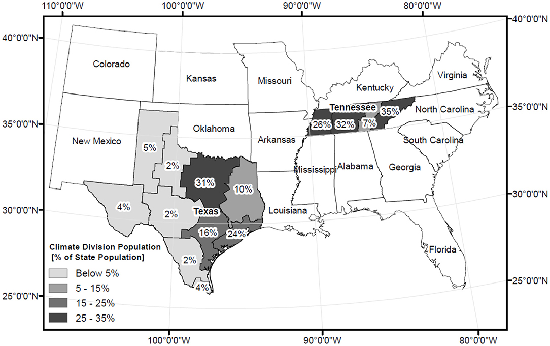
Figure 1. Map of the climate divisions in Tennessee and Texas. The color of the climate division indicates the average percentage of the state population in each climate division for the timeframe of this study. Darker colors represent a higher percentage.

The meteorological conditions at both states differ significantly during the year. While TN has a mean of 5.8°C (42.5°F) during the winter season and 23.4°C (74.05°F) during the summer season, TX has 12.1°C (53.84°F) in the winter and 27.5°C (81.46°F) in the summer, respectively. The temperature variability is more pronounced in TN that has a coefficient of variation of 0.146 during the winter and 0.053 during the summer, while TX presents a coefficient of variation of 0.10 during the winter and 0.04 during the summer.

Temperature Forecasts Database

To investigate the potential in forecasting monthly power demands during winter and summer over the two states, we utilize the retrospective monthly temperature forecasts from ECHAM4.5 (Li and Goddard, 2005) and NOAA's Climate Forecast System (CFS) (Saha et al., 2006) obtained from the International Research Institute of Climate and Society (IRI) data library, which have good skills in forecasting surface temperature in the U.S. and have long retrospective forecasts available from 1960. Temperature forecasts from ECHAM4.5, an atmospheric general circulation model (GCM), was obtained by forcing it with 3-month ahead sea-surface temperature (SST) forecasts obtained using the constructed analog method from Van Den Dool (1994). CFS is a coupled GCM between ocean and atmosphere and it provides both retrospective and real-time temperature forecasts starting in 1957. For 3-month ahead forecasts, we averaged the gridded temperature forecasts over each state to obtain JFM (JAS) monthly time series of temperature forecasts issued at the beginning of January (July) for the period 1990–2015. Temperature forecasts from both models are available at 2.5° grid points, and to obtain the state temperature forecast for each state, we will spatially average the forecasts for grid points within each state. For forecasts, we did not consider population-weighted temperature since they are available at large-spatial scale. Given the population-weighted temperature and the forecast temperature exhibit strong correlation (Table 1), its ability in explaining the power demand variability remained good. For Texas, we used the coordinates (34.307144, −103.011246) for the northwest corner and (29.764377, −94.397964) for the southeast corner. For Tennessee, we used (36.465472, −89.529305) for the northwest corner and (35.003003, −84.364872) for the southeast corner. In this study, we utilize the forecasted ensemble mean from each GCM, which is obtained by computing the average over their respective ensembles to obtain 3-month ahead temperature forecasts for the winter and summer seasons over the period 1990–2015.

TABLE 1

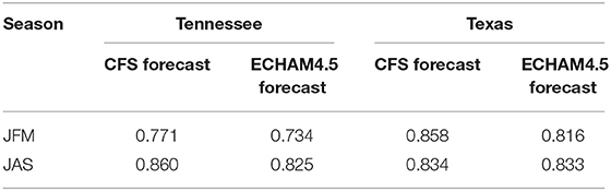
Table 1. Correlation between observed population weighted average temperature and forecasted average temperature from two atmospheric GCM forecasts, CFS and ECHAM 4.5, for the winter and summer seasons.

Natural Gas Consumption

We also considered natural gas consumption as a potential variable for residential heating loads that could replace electricity for heating. Monthly consumption of natural gas consumption was obtained from the EIA for the period 1990–2015 (Energy Information Administration, 2019).

Results and Discussion

Relationship Between Population and Electricity Demand

Since we are explaining the variability in power demand over a 26 year period, we expect population to be the primary driver of electricity demand. This is indicated by the linear trend (Figure 2) between the population and electricity demand during the winter and summer seasons by the two systems. For TN, the coefficient of determination between the population and the electricity demand during the winter (summer) was 0.40 (0.68), whereas for the TX system, the population explained 0.66 (0.74) of the variability in electricity demand during the winter (summer) season. Even though the variability explained by population is statistically significant at a 95% confidence level, unexplained variance in the electricity demand could be due to other factors, such as industrial growth and other development. We also considered each State's Gross Domestic Product (GDP) as another explanatory variable for electricity demand variability over the study period (Supplementary Figure 1). However, we found the explained variability by both population growth and GDP were almost the same, since correlation between GDP and population growth was very high. Results for the regression of electricity demand and GDP are presented in the Supplementary Material, and as can be noticed the variability explained by GDP is lesser than population. Hence, we decided to consider population growth as the primary variable for obtaining the residuals, since monthly population values could be better interpolated based on annual population.

FIGURE 2

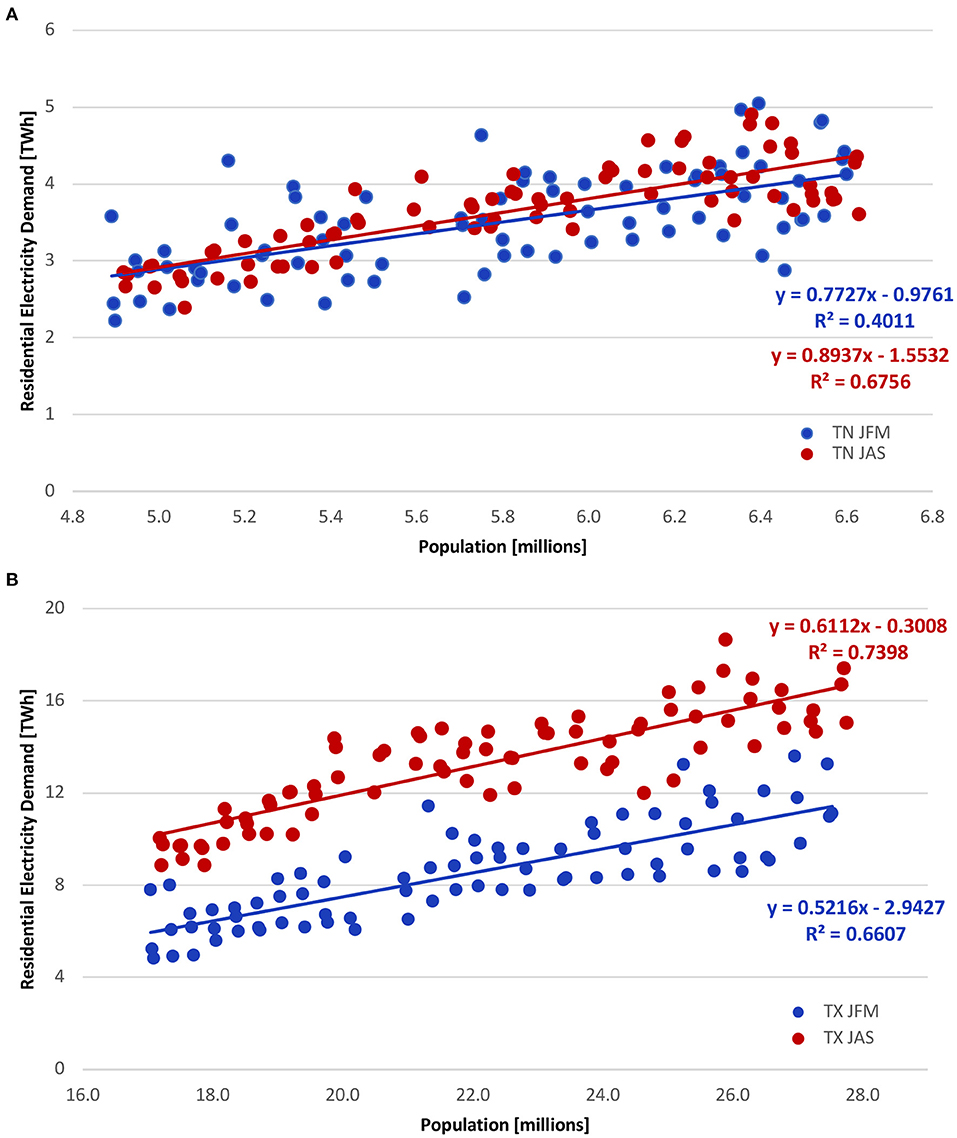
Figure 2. Scatterplot of population from 1990 to 2015 in millions and the observed electricity demand (TWh) for the (A) Tennessee and (B) Texas power systems. Winter JFM (summer JAS) months are represented in blue (red) circles with the trend line (blue or red) for each season indicating the explained variability on the electricity demand.

The Role of Temperature to Explain the Interannual Variability in Electricity Demand

We hypothesize that the unexplained variance in electricity demand could be partially explained by the interannual variation in seasonal temperature. To evaluate this hypothesis, we obtained the monthly residuals between the electricity demand and population from Figure 2 during the winter and summer seasons for the TX and TN systems. Figure 3 shows the scatterplot of monthly residuals with observed monthly population-weighted average temperature for the winter (summer) season for both systems. For TN, the monthly population weighted average temperature explained 63% (44%) of the monthly residual variance remaining from the regression of electricity demand and population growth for the winter (summer) season. We multiplied the unexplained variance from the population-electricity demand regression (Figure 2) by the explained variance from the residual-population weighted average temperature regression (Figure 3) to estimate the total variance explained by temperature on seasonal electricity demand. For the TN system, the population weighted temperature explained an additional 38% (i.e., [1–0.40] (Figure 2A)^* 0.63 (Figure 3A)) of the interannual variability in the winter electricity demand. Similarly, considering population weighted temperature explained an additional 14% of the variability in the TN summer electricity demand. From Figures 3C,D for the TX system, the R² between residuals was 67% (46%) for the winter (summer) season. Thus, considering the population weighted average temperature explained an additional 23% (12%) of the interannual variability in TX electricity demand. We also performed a similar analysis to identify the role of population and weighted average temperature in residential electricity demand for both states. The results were very similar to those above, and thus omitted.

FIGURE 3

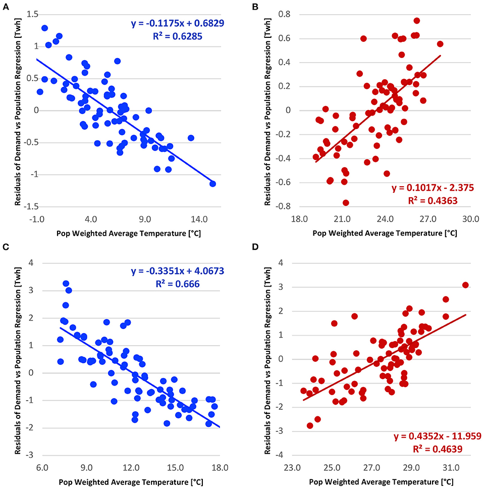
Figure 3. Scatter plots of residuals from the regression between electricity demand and population with observed monthly population weighted average temperature for (A) TN winter, (B) TN summer, (C) TX winter, and (D) TX summer. Residuals corresponding to winter (summer) months are indicated in blue (red) circles.

In the case of the TX system, we observe that temperature explains more variability in both the winter and summer electricity demand. This is partly due to increased interannual variability in the seasonal temperature for the TX system. From the perspective of developing electricity demand forecasts for the upcoming season, any variability around the projected demand will be predominantly due to potential changes in seasonal average daily minimum/maximum temperature, which in turn affect heating/cooling loads. Thus, from Figure 3, considering population weighted average temperature could provide information that helps explain the variability in electricity demand. From a seasonal planning and management perspective, the potential information on changes in electricity demand due to the variability in temperature could help utilities to properly stockpile fuel and schedule maintenance of existing power generation plants.

Potential to Forecast Seasonal Electricity Demand Using GCM Temperature Forecasts

We also evaluated the potential in developing season-ahead power demand forecasts using the forecasted temperature from two GCMs, ECHAM4.5 and CFS, for the TX and TN systems. Several studies have evaluated the skill in predicting seasonal temperature forecasts and found that the skill in predicting the interannual variation in temperature is in general higher than the one obtained when predicting the precipitation over many parts of the continental US (e.g., Goddard et al., 2003; Devineni and Sankarasubramanian, 2010a,b). Table 1 shows the correlation between the observed average temperature and the forecasted average temperature for the two systems during the winter and summer seasons. The computed correlations are statistically significant at a 95% confidence level (±1.96/√n−3, where “n” denotes the number of data points used to calculate the correlation). Table 1 indicates that the skill of temperature forecasts from both GCMs in predicting the population weighted temperature is statistically significant at a 95% confidence interval even though the forecasts are spatially averaged rather than population weighted. Figures 4, 5 show the skill of temperature forecasts in explaining the residuals obtained between electricity demand and population growth. From both figures, we can infer that the skill of forecasted temperature in predicting interannual electricity demand variations is similar to that when observed temperature is used instead (Figure 3). Further, the skill exhibited by the CFS model is in general higher than the skill exhibited by the ECHAM4.5 in predicting the interannual variations in the residuals between electricity demand and population growth. The skill associated with temperature forecasts presented in Figures 4, 5 are higher in general for the winter than in the summer. This is consistent with the better ability to predict/forecast winter precipitation and temperature than in the summer, since the seasonal climate is more influenced by the ENSO-related variability (Goddard et al., 2003). Also, summer climate is more influenced by local disturbances, whereas winter climate is influenced by structured low-frequency oscillations (Goddard et al., 2003; Devineni and Sankarasubramanian, 2010a,b). Table 2 presents the root mean square error of the regression between electricity demand vs. population and temperature forecasts from GCMs, where results are between 71.2–76.3% for Tennessee and 80.4–88.4% for Texas. This analysis shows the ability of GCM forecasts in predicting the power demand for the two seasons in both states.

FIGURE 4

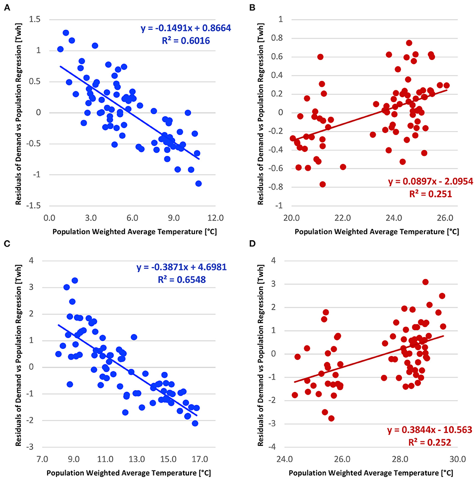
Figure 4. Ability of the bias-corrected CFS seasonal average temperature forecast to explain the interannual variability of residuals obtained from the regression between observed electricity demand and population: (A) TN JFM, (B) TN JAS, (C) TX JFM, and (D) TX JAS. Residuals corresponding to winter (summer) months are indicated in blue (red) circles.

FIGURE 5

Figure 5. Ability of the bias-corrected ECHAM4.5 seasonal average temperature forecast to explain the interannual variability of residuals obtained from the regression between observed power demand and population: (A) TN JFM, (B) TN JAS, (C) TX JFM, and (D) TX JAS. Residuals corresponding to winter (summer) months are indicated in blue (red) circles.

TABLE 2

Table 2. Root mean square error in the predicted power demand from the regression against population and GCM forecasted temperature.

Discussion and Remarks

Findings from Figures 2–5 show that both observed and forecasted temperature significantly explain the interannual variability in electricity demand residuals, which were obtained by regressing the electricity demand against the population served. This indicates that population growth in a region plays an important role in explaining the variability in electricity demand at decadal time scales, whereas temperature has a significant effect on electricity demand variability at seasonal time scales. Numerous studies have developed seasonal streamflow forecasts using seasonal precipitation forecasts from GCMs (Maurer and Lettenmaier, 2003; Oludhe et al., 2013; Sinha and Sankarasubramanian, 2013). Studies have also shown that the skill in predicting seasonal temperature is much higher than that of precipitation (Goddard et al., 2003; Devineni and Sankarasubramanian, 2010a). Given the similar level of variability in explaining the power demand by both observed and forecasted temperature, this study underscores the potential for developing seasonal electricity demand forecasts contingent on temperature forecasts from GCMs. To begin with, simple low-dimensional empirical models that utilize the principal components of temperature forecasts could be used to develop electricity demand forecasts. Multi-model temperature forecasts can also be used to develop electricity demand forecasts since it reduces the uncertainty associated with a particular GCM and can lead to a better calibrated forecast (Goddard et al., 2003; Devineni and Sankarasubramanian, 2010a), and future studies could explore that in the context of seasonal power demand forecasting.

Studies utilizing streamflow forecasts derived from seasonal climate forecasts have clearly improved reservoir management, particularly hydropower generation, over the status quo use of climatology (i.e., no forecasts) (Sankarasubramanian et al., 2009a; Oludhe et al., 2013). Thus, developing electricity demand forecasts along with streamflow forecasts at seasonal time scales could potentially lower the cost of electric dispatch in at least five ways: (1) operational planning for generation and transmission systems, (2) projecting the need for emissions allowances in coming months, (3) forward purchases of fuel reserves (e.g., coal stock piles), (4) demand response planning, and (5) hydroelectric release planning. Thus, the information available from electricity demand forecasts and streamflow forecasts could be used within power system and reservoir management models to minimize the cost of power generation. Studies have shown that the utility of forecasts increases as the demand increases under a given reservoir system capacity (Maurer and Lettenmaier, 2003; Sankarasubramanian et al., 2009b). In a similar context, as the electricity demand increases, the availability of demand forecasts is expected to facilitate improved power system operation (Sankarasubramanian et al., 2014). In addition, as the U.S. power system continues to decarbonize, an increasing share of electricity demand will likely be met by variable renewables. Under such conditions, electricity supply—in addition to demand—will become increasing dependent on the prevailing meteorological and climatic conditions. As such it will become increasing important to improve the linkage between forecasted seasonal climate and electricity supply and demand.

This work did not explicitly attribute the role of efficiency in power demand consumption in explaining the interannual variability in the winter and summer demand for the two states since we did not find any temporal trend in the power demand residual obtained after regressing with the population. With increased data availability, if the efficiency in the power demand is significant as in Greening et al. (2000), then it could be explicitly incorporated by considering the previous year demand as a predictor as in Wang et al. (2017). Hence, for our analysis with the two states, efficiency in power consumption did not play any substantial role. Nonetheless, we attempted to use the previous month demand as a predictor of the residual of the analysis after the regression with respect to the temperature. This additional predictor in TN had a coefficient of determination of 1% (13%) in the winter (summer), and in TX the same predictor had a coefficient of determination of 1% (5%) in the winter (summer) (Supplementary Figure 2).

In the winter season, we found that residential natural gas (NG) consumption plays a role in explaining the variability and it was included as a predictor for both TN and TX. For both states, the natural gas consumption explained 8% (TN) and 10% (TX) variability as a substitution effect in accounting winter heating loads (Supplementary Figure 3). During the summer, NG was not significant because it is not used as a source for cooling, hence the explained variability was very low (not reported for brevity). The final resulting residual diagnostic plots (Supplementary Figure 4) for winter and summer show the residuals are normally distributed based on the reported skewness of the residuals.

Conclusion

This work presented a framework to assess the role of temperature variability on explaining seasonal residential electricity demand and it was applied to analyze two Southern states in the US. The methodology is based on regression analysis and employs population, temperature forecasts from general circulation models, natural gas consumption, and previous month electricity demand as predictors of the monthly residential electricity demand. Results from the analysis carried out indicate that regional population growth explains most of the residential electricity demand variability at longer time scales (i.e., 10–20 years), whereas temperature explains 44–67% of the electricity demand variability at seasonal time scales. We have also assessed the use of seasonal temperature forecasts from general circulation models to develop season-ahead power demand forecasts. Results suggest that the root mean square error in the predicted power demand from the regression against population and GCM forecasted temperature are between 71.2–76.3% (Tennessee) and 80.4–88.4% (Texas). Therefore, the approach combined with the analysis presented here suggest that the use of climate forecasts can potentially help to project future residential electricity demand at monthly to seasonal time scale.

Findings from this study also provide a basis for setting up adaptive management of power systems contingent on seasonal climate information by continuously developing monthly electricity demand forecasts based on the monthly updated climate forecasts. While this study considered two largely self-contained systems, the approach presented here could be used to analyze electricity demand in other states and countries. This paper has also focused on providing an understanding about the effects of seasonal climate variability in power demand using other predictor variables, such as population and natural gas consumption. Future works could explore additional predictors, such as electricity prices and energy efficiency for estimating future power demand. We also note that, while temperature was considered at different climatic areas within the states analyzed, data for monthly electricity demand was not available as disaggregate information. As new disaggregate demand data becomes available, future studies could explore the development of different forecasting models for each climatic region. Finally, future studies could also investigate the use of other forecasting methods including deep neural networks, random forest, Bayesian hierarchical models and others.

Data Availability Statement

Publicly available datasets were analyzed in this study. This data can be found at: https://www.eia.gov/electricity/data.

Author Contributions

AS designed the research. DC and AQ performed the research. DC, HE, AQ, and AS contributed the analytic tools. DC and HE analyzed the data. DC, HE, AQ, AS, and JD wrote the paper. All authors contributed to the article and approved the submitted version.

Funding

This material was based upon work supported by the National Science Foundation CAREER grants CBET-0954405 and CBET-1055622 and CCF 1442909. Any opinions, findings, and conclusions or recommendations expressed in this paper are those of the authors and do not reflect the views of the NSF.

Conflict of Interest

The authors declare that the research was conducted in the absence of any commercial or financial relationships that could be construed as a potential conflict of interest.

Supplementary Material

The Supplementary Material for this article can be found online at: https://www.frontiersin.org/articles/10.3389/frsc.2021.644789/full#supplementary-material

References

Auffhammer, M., Baylis, P., and Hausman, C. H. (2017). Climate change is projected to have severe impacts on the frequency and intensity of peak electricity demand across the United States. Proc. Natl. Acad. Sci. U.S.A. 114, 1886–1891. doi: 10.1073/pnas.1613193114

PubMed Abstract | CrossRef Full Text | Google Scholar

Bartos, M. D., and Chester, M. V. (2015). Impacts of climate change on electric power supply in the western United States. Nat. Clim. Change 5, 748–752. doi: 10.1038/nclimate2648

CrossRef Full Text | Google Scholar

Burillo, D., Chester, M. V., Ruddell, B., and Johnson, N. (2017). Electricity demand planning forecasts should consider climate non-stationarity to maintain reserve margins during heat waves. Appl. Energy 206, 267–277. doi: 10.1016/j.apenergy.2017.08.141

CrossRef Full Text | Google Scholar

Changnon, S. A., Changnon, J. M., and Changnon, D. (1995). Uses and applications of climate forecasts for power utilities. Bull. Am. Meteorol. Soc. 76, 711–720. doi: 10.1175/1520-0477(1995)076<0711:UAAOCF>2.0.CO;2

CrossRef Full Text | Google Scholar

Changnon, S. A., and Kunkel, K. E. (1999). Rapidly expanding uses of climate data and information in agriculture and water resources: causes and characteristics of new applications. Bull. Am. Meteorol. Soc. 80, 821–830. doi: 10.1175/1520-0477(1999)080<0821:REUOCD>2.0.CO;2

CrossRef Full Text | Google Scholar

Changnon, S. D. (2003). Measures of economic impacts of weather extremes: getting better but far from what is needed—a call for action. Bull. Am. Meteorol. Soc. 84, 1231–1236. doi: 10.1175/BAMS-84-9-1231

CrossRef Full Text | Google Scholar

Chilkoti, V., Bolisetti, T., and Balachandar, R. (2017). Climate change impact assessment on hydropower generation using multi-model climate ensemble. Renew. Energy 109, 510–517. doi: 10.1016/j.renene.2017.02.041

CrossRef Full Text | Google Scholar

De Felice, M., Alessandri, A., and Catalano, F. (2015). Seasonal climate forecasts for medium-term electricity demand forecasting. Appl. Energy 137, 435–444. doi: 10.1016/j.apenergy.2014.10.030

CrossRef Full Text | Google Scholar

De Queiroz, A. R., Lima, L. M. M., Lima, J. W. M., Silva, B. C., and Scianni, L. A. (2016). Climate change impacts in the energy supply of the Brazilian hydro-dominant power system. Renew. Energy 99, 379–389. doi: 10.1016/j.renene.2016.07.022

CrossRef Full Text | Google Scholar

Devineni, N., and Sankarasubramanian, A. (2010a). Improved categorical winter precipitation forecasts through multimodel combinations of coupled GCMs. Geophys. Res. Lett. 37, 1–22. doi: 10.1029/2010GL044989

CrossRef Full Text | Google Scholar

Devineni, N., and Sankarasubramanian, A. (2010b). Improving the prediction of winter precipitation and temperature over the continental United States: role of ENSO state in developing multimodel combinations. Mon. Weather Rev. 138, 2447–2468. doi: 10.1175/2009MWR3112.1

CrossRef Full Text | Google Scholar

Energy Information Administration (2015). Form EIA-826 Detailed Electricity Consumption Data. Available online at: http://www.eia.gov/electricity/data/eia826/ (accessed December 22, 2015).

Energy Information Administration (2019). Natural Gas Consumption by End Use. Available online at: https://www.eia.gov/dnav/ng/ng_cons_sum_a_EPG0_vrs_mmcf_m.htm (accessed November 14, 2019).

Google Scholar

Franco, G., and Sanstad, A. H. (2008). Climate change and electricity demand in California. Clim. Change 87, 139–151. doi: 10.1007/s10584-007-9364-y

CrossRef Full Text | Google Scholar

Frank, T. (2005). Climate change impacts on building heating and cooling energy demand in Switzerland. Energy Build. 37, 1175–1185. doi: 10.1016/j.enbuild.2005.06.019

CrossRef Full Text | Google Scholar

Gaterell, M. R., and McEvoy, M. E. (2005). The impact of climate change uncertainties on the performance of energy efficiency measures applied to dwellings. Energy Build. 37, 982–995. doi: 10.1016/j.enbuild.2004.12.015

CrossRef Full Text | Google Scholar

Goddard, L., Barnston, A. G., and Mason, S. J. (2003). Evaluation of the IRI's “net assessment” seasonal climate forecasts: 1997–2001. Bull. Am. Meteorol. Soc. 84, 1761–1781. doi: 10.1175/BAMS-84-12-1761

CrossRef Full Text | Google Scholar

Greening, L. A., Greene, D. L., and Difiglio, C. (2000). Energy efficiency and consumption—the rebound effect—a survey. Energy Policy 28, 389–401. doi: 10.1016/S0301-4215(00)00021-5

CrossRef Full Text | Google Scholar

Holmes, M. J., and Hacker, J. N. (2007). Climate change, thermal comfort and energy: meeting the design challenges of the 21st century. Energy Build. 39, 802–814. doi: 10.1016/j.enbuild.2007.02.009

CrossRef Full Text | Google Scholar

Hor, C., Watson, S. J., and Majithia, S. (2005). Analyzing the impact of weather variables on monthly electricity demand. IEEE Trans. Power Syst. 20, 2078–2085. doi: 10.1109/TPWRS.2005.857397

CrossRef Full Text | Google Scholar

IPCC Climate Change (2013). The Physical Science Basis. Contribution of Working Group I to the Fifth Assessment Report of the Intergovernmental Panel on Climate Change. Cambridge and New York, NY: Cambridge University Press.

Google Scholar

Isaac, M., and Vuuren, D. P. (2009). Modeling global residential sector energy demand for heating and air conditioning in the context of climate change. Energy Policy 37, 507–521. doi: 10.1016/j.enpol.2008.09.051

CrossRef Full Text | Google Scholar

Li, S., and Goddard, L. (2005). Retrospective Forecasts with the ECHAM4.5 AGCM. IRI Technical Report 05-02. New York, NY: The Earth Institute, Columbia University. Available online at: http://iri.columbia.edu/outreach/publication/report05–02/report05–02.pdf

Google Scholar

Maurer, E. P., and Lettenmaier, D. P. (2003). Predictability of seasonal runoff in the Mississippi River basin. J. Geophys. Res. Atmos. 108, 2-1–2-13. doi: 10.1029/2002JD002555

CrossRef Full Text | Google Scholar

Mirasgedis, S., Sarafidisa, Y., Georgopouloua, E., Lalasa, D. P., Moschovits, M., Karagiannis, F., et al. (2006). Models for mid-term electricity demand forecasting incorporating weather influences. Energy 31, 208–227. doi: 10.1016/j.energy.2005.02.016

CrossRef Full Text | Google Scholar

Mukhopadhyay, S., and Nateghi, R. (2017). Climate sensitivity of end-use electricity consumption in the built environment: an application to the state of Florida, United States. Energy 128, 688–700. doi: 10.1016/j.energy.2017.04.034

CrossRef Full Text | Google Scholar

National Research Council (2010). Advancing the Science of Climate Change. Washington, DC: The National Academies Press.

Google Scholar

NOAA (2016). National Centers for Environmental Information (Formally National Climatic Data Center). Available online at: http://www.ncdc.noaa.gov/monitoring-references/maps/us-climate-divisions.php

Oludhe, C., Sankarasubramanian, A., Sinha, T., Devineni, N., and Lall, U. (2013). The role of multimodel climate forecasts in improving water and energy management over the Tana River Basin, Kenya. J. Appl. Meteorol. Climatol. 52, 2460–2475. doi: 10.1175/JAMC-D-12-0300.1

CrossRef Full Text | Google Scholar

Pardo, A., Meneu, V., and Valor, E. (2002). Temperature and seasonality influences on Spanish electricity load. Energy Econ. 24, 55–70. doi: 10.1016/S0140-9883(01)00082-2

CrossRef Full Text | Google Scholar

Reyna, J. L., and Chester, M. V. (2017). Energy efficiency to reduce residential electricity and natural gas use under climate change. Nat. Commun. 8:14916. doi: 10.1038/ncomms14916

PubMed Abstract | CrossRef Full Text | Google Scholar

Ronalds, B. F., Wonhas, A., and Troccoli, A. (2010). “A new era for energy and meteorology,” in Weather Matters for Energy, eds A. Troccoli, L. Dubus and S. E. Haupt (New York, NY: Springer), 3–16. doi: 10.1007/978-1-4614-9221-4_1

CrossRef Full Text | Google Scholar

Saha, S., Nadiga, S., Thiaw, C., Wang, J., Wang, W., Zhang, Q., et al. (2006). The NCEP climate forecast system. J. Clim. 19, 3483–3517. doi: 10.1175/JCLI3812.1

CrossRef Full Text | Google Scholar

Sailor, D. J., and Munoz, J. R. (1997). Sensitivity of electricity and natural gas consumption to climate in the U.S.A. Methodology and results for eight states. Energy 22, 987–998. doi: 10.1016/S0360-5442(97)00034-0

CrossRef Full Text | Google Scholar

Sailor, D. J., and Pavlova, A. A. (2003). Air conditioning market saturation and long-term response of residential cooling energy demand to climate change. Energy 28, 941–951. doi: 10.1016/S0360-5442(03)00033-1

CrossRef Full Text | Google Scholar

Sankarasubramanian, A., Lall, U., Devineni, N., and Espunevea, S. (2009a). Utility of operational streamflow forecasts in improving within-season reservoir operation. J. Appl. Climatol. Meteorol. 48, 1464–1482. doi: 10.1175/2009JAMC2122.1

CrossRef Full Text | Google Scholar

Sankarasubramanian, A., Lall, U., Souza Filho, F. A., and Sharma, A. (2009b). Improved water allocation utilizing probabilistic climate forecasts: short term water contracts in a risk management framework. Water Resour Res. 45:W11409. doi: 10.1029/2009WR007821

CrossRef Full Text | Google Scholar

Sankarasubramanian, A., Lu, N., Mahinthakumar, G., DeCarolis, J., and Sreepathi, S. (2014). Cybersees Type 2: Cyber-Enabled Water and Energy Systems Sustainability Utilizing Climate Information. Award # 1442909. Available online at: http://www.nsf.gov/awardsearch/showAward?AWD_ID=1442909

Sinha, T., and Sankarasubramanian, A. (2013). Role of climate forecasts and initial land-surface conditions in developing operational streamflow and soil moisture forecasts in a rainfall-runoff regime: skill assessment. Hydrol. Earth Syst. Sci. 17, 721–733. doi: 10.5194/hess-17-721-2013

CrossRef Full Text | Google Scholar

US Census Bureau (2015). Population and Housing Unit Estimates. Available online at: http://www.census.gov/popest/index.html (accessed December 22, 2015).

Van Den Dool, H. M. (1994). Searching for analogues, how long must we wait? Tellus A 46, 314–324. doi: 10.1034/j.1600-0870.1994.t01-2-00006.x

CrossRef Full Text | Google Scholar

Wang, S., Sun, X., and Lall, U. (2017). A hierarchical Bayesian regression model for predicting summer residential electricity demand across the USA. Energy 140, 601–611. doi: 10.1016/j.energy.2017.08.076

CrossRef Full Text | Google Scholar