Is ward-level calculation of urban green space availability important?—A case study on Vellore city, India, using the histogram-based spectral discrimination approach

1 Introduction

Developing countries, such as India, have witnessed rapid growth in the majority of their cities over the last two decades due to the migration of people from village to cities in search of better job opportunities and an improved lifestyle. It is predicted that the country’s population will increase by 310 million in the next 15 years, and the share of urban population alone would be approximately 220 million, accounting for more than 70% of the total increase (MoHFW, 2020). One of the major effects of urbanization that has a profound environmental and social impact on a city is the loss of green cover. Urban green space (UGS), which is popularly known in literature, is defined as the area which is covered by vegetation that normally includes trees, crop lands, and shrubs and these spaces are considered as the last vestiges of nature in urban areas (Sathyakumar et al., 2020; Sun et al., 2022). The presence of a sufficient quantity of UGS in cities is important from an environmental and ecological point of view as UGS helps to reduce urban heat island (UHI) effects, improve the air and water quality, prevent soil erosion, reduce the risk of flooding, and improve the biodiversity (Kowe et al., 2021; Kefale et al., 2023; Lind et al., 2023). In addition to many environmental and ecological benefits, UGS also offers many social advantages. For example, it provides a pleasant environment for walking and engaging in physical exercises, which leads to low stress levels (Semeraro et al., 2021; Li et al., 2023; Rehman et al., 2024). It also provides increased recreational opportunities and strengthens neighborhood relationships (Farkas et al., 2023). As there are many benefits associated with UGS, several countries in the world have stipulated guidelines on how much green space should be available in a city on per capita and/or geographical area basis. For example, a city should have UGS in the range of 9–50 m²/person, or 20–40% of the city’s geographical area must be covered in green (Ramaiah and Avtar, 2019; NITI Aayog, 2021; Roy and Fleischman, 2022).

Google Earth (GE), one of the popular remote sensing data sources, can be used to extract various green cover types such as trees, shrubs, grasslands, and croplands as it contains very high-resolution satellite images. Several studies have reported the use of GE in various applications such as mapping of mangrove species (Li et al., 2020), geomorphological landforms (Datta and Sarkar, 2019), detonation destruction (Kumar et al., 2022), landslide susceptibility (Li et al., 2022), coastal aquaculture (Kurekin et al., 2022), and urban settlement mapping (Emeterio and Mering, 2021). Although there are many studies reported in other fields, studies on the use of GE images for UGS extraction are very limited (Sun et al., 2020; Markovic et al., 2021). Most of the researchers have used GE images only for assessing the accuracy of the UGS map prepared using low- and medium-resolution satellite data such as Landsat TM and ETM+ and did not use GE images as a direct data source to prepare the UGS map, though one can clearly distinguish various UGS types in GE images (Kuang and Dou, 2020; Sun et al., 2020; Markovic et al., 2021). Some authors have performed manual digitization of UGS using the GE images in the background; however, it is a very cumbersome and time-taking process (Lahoti et al., 2019). To overcome the above-mentioned drawbacks, the present study has proposed a two-step approach, where the histograms of red, green, and blue bands of GE images were analyzed first to check whether the green cover types are spectrally different or not. Then, the classification methods were applied, and accuracy assessment was performed to identify the best suitable method for automatic extraction of UGS from GE images. The availability of adequate green space in a city is a major concern for planners and policymakers, and the present study aimed to address this issue through two approaches: one based on the per capita and the other one based on the geographical area by utilizing UGS data extracted through the proposed histogram-based spectral discrimination approach. In most of the studies, UGS was calculated based on the population or geographical area but at the macro level, i.e., for the city as a whole (Badiu et al., 2016; Hwang et al., 2020) or at the district level (Pouya and Majid, 2022). Only limited studies were carried out at micro- or ward-level for analysis (Shekhar and Aryal, 2019). As we can easily obtain ward-wise population information based on electoral rolls, the same can be used to calculate ward-wise UGS per capita. The results would be useful to find out the wards where UGS is surplus or deficit, and such information would help the civic authorities in developing action plans to improve the greenery in wards where UGS is deficit. Although we can utilize the GE images for UGS extraction and mapping, we can only calculate the areal extent of UGS at a two-dimensional scale, and information at the individual tree level is not possible. To overcome this limitation, the present study has explored the three-dimensional LiDAR data to obtain green space information at the individual tree level, including attributes such as height, diameter, and crown area. The temperature of trees was also calculated using LiDAR data and compared with the temperature of adjacent buildings and roads, to determine whether green space is beneficial in lowering the temperature of the surrounding. The objectives of the present study are (1) to perform histogram-based spectral discrimination and classification of green cover types using Google Earth images, (2) to calculate how much green space is actually available for individuals based on per capita and geographical area and compare it with the standards (3), To utilize 3D LiDAR data to extract information at the individual tree level and check whether green space is beneficial in lowering the temperature of the surrounding.

2 Materials and methods

2.1 Details about the study area

Vellore Corporation, which is the administrative headquarter of Vellore district, is selected as the study area for the present research work and a map of the same is shown in Figure 1C. It is located on the northern part of Tamil Nadu state in India, as shown in Figure 1B. It spreads over an area of 95.52 km² (Figure 1C) and has a population of nearly 0.4 million. Vellore has a well-connected road network with two major national highways (NH), NH-48 and NH-234, passing through it. In addition, it is well connected by the railway network to all major stations in the country. Though Vellore is one of the preferred locations for tourism and education, the only drawback in the city is the high temperature that prevails during the summer season. It is one of the hottest cities in the state with temperature shooting up to 42°C in summer months such as April–May. One way to reduce these heat islands is to have more green cover in the city, and in order to achieve it, thousands of saplings are planted every year and many parks have been constructed in and around the Vellore city. The assessment of prevailing green cover in the city through GE images and LiDAR data would not only help authorities to check whether the city has met the nation’s standards on green cover but also help to identify the open spaces which can possibly be converted to UGS in future.

Figure 1

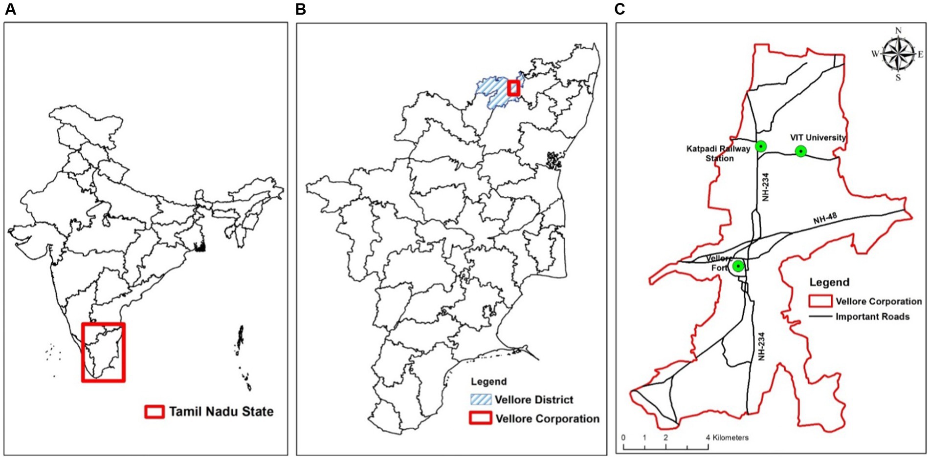
Figure 1. Map showing (A) Tamil Nadu state in India, (B) Vellore district and Vellore corporation in Tamil Nadu state, (C) Study area of Vellore Corporation.

2.2 Data used

The present study is based on the Google Earth (GE) satellite images, and the first step is to check for the availability of satellite imagery which is free from clouds because even a small patch of clouds in the GE image may affect the classification results. Finally, the cloud-free GE images covering the study area of Vellore, India, were downloaded using an open-source software, namely, the “Smart GIS” (Elshayal, 2023). The maximum possible zoom level was set in software, and the GE images covering the study area were then downloaded. A total of 496 tiles of GE images which have a size of approximately 4.75 GB were finally downloaded. The downloaded images were then pieced together to form one single image, which was clipped within the Vellore Corporation. The downloaded image was in geographic coordinate system (decimal degrees), and the same was converted to projected coordinate system (m) in ArcMap using Universal Transverse Mercator (UTM) projection zone 44 N. The pixel size of the clipped image was found to be 0.53 × 0.53 m, which indicates that the images from GE are of very high resolution. The true color composite (TCC) of the projected GE image is shown in Figure 2. As evident from Figure 2, one can clearly identify the green cover types such as trees, grassland, and crop land in the GE image. It is necessary to check whether the red (R), green (G), or blue (B) values of pixels covering these green areas differ from each other and also from other land covers such as buildings, roads, and water so that we can differentiate UGS from other land covers in the GE image and easily extract it. The procedure to check the same is explained in the following section.

Figure 2

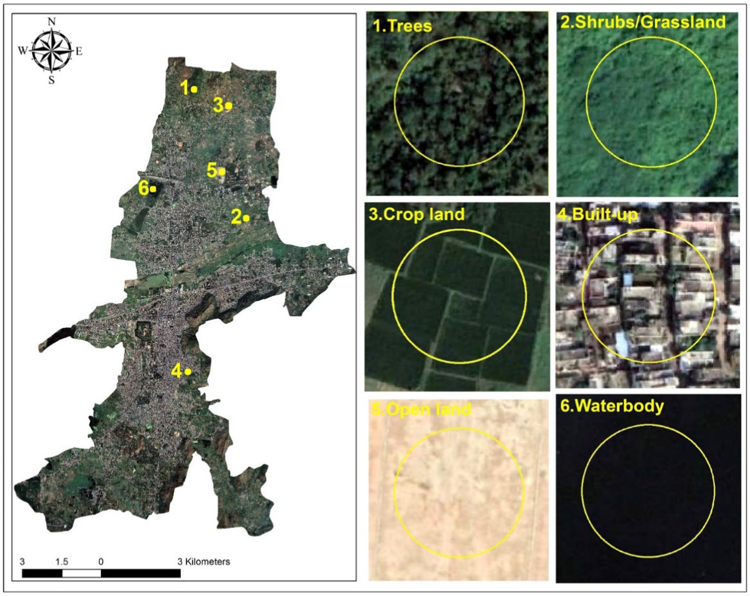
Figure 2. True color composite of the GE image (left) and the six representative classes (right).

2.3 Histogram-based spectral discrimination analysis to check the applicability of GE image for UGS extraction

Before calculating the histograms, it is necessary to first identify the representative areas for each class from the GE image and then plot the histogram for each of its bands (R, G, and B) from the selected representative area. A total of six classes were taken, namely, trees, shrubs/grassland, crop land, built-up, open land, and water bodies. Among the six classes, the first three will come under UGS and the remaining are named as “others.” For each class, a representative area was identified in the GE image. A point was placed on the center of the representative area (for example, crop land), and then, a buffer was created for a radius of 30 m. The GE image within the buffer was then clipped for all the six representative classes, as shown in Figure 2. For each buffered image, three images corresponding to R, G, and B bands were obtained, with each band having 10,216 pixels. By using the pixel values and their corresponding count (number of pixels with the same pixel value), the histograms were then plotted. A total of 18 histograms were plotted as there were 6 classes with 3 bands in each. The histograms were then analyzed to check whether any significant difference existed among them. If any significant difference is found between the histograms of each class, it indicates that the image classification methods can be applied to the GE image to extract the UGS as the pixel values of UGS differ from each other (trees, shrubs/grassland, and crop land) and also from other land cover classes. Once the first step of the histogram analysis to find the suitability of GE images for UGS extraction was over, the next step of image classification was performed as explained below.

2.4 Details of UGS classification methods and calculation of available UGS

Popular image classification methods such as supervised, unsupervised, and object-based were used to classify the GE images into four classes, namely, trees, shrubs/grassland, crop land, and others (built-up, open land, and water bodies). Each of these classification methods has been briefly explained below. For supervised classification, two popular methods, namely, support vector machine (SVM) and maximum likelihood (ML) were applied using the “Image Classification” toolbar of ArcGIS software. For supervised classification, it is essential to give the training polygons for each land cover class considered, and generally, it is recommended to use 15–20 polygons for each class (ESRI, 2023). In the present study, 60 polygons, which is three times more than the recommended amount, were given for each class, namely, trees, shrubs/grassland, crop land, built-up, open land, and water bodies. In the SVM method, once the GE image and the training polygons were provided as input, the classifier tool generated an ESRI Classifier Definition (.ecd) file, which was then used again with the GE image to obtain the final classified image with six classes. This process took almost 4 h as the image is of a very high resolution with training polygons which contain approximately 2.1 billion pixels. Once the classified image was classified, it was then reclassified into four classes, namely, trees, shrubs/grassland, crop land, and others, as the study focused mainly on UGS extraction. The reclassified raster image was then used for accuracy assessment using 300 points randomly distributed throughout the study area. According to Congalton and Green (2019), 50 random points per land use/land cover class are generally sufficient for accuracy assessment. As the reclassified output has 4 classes, 200 points may be sufficient; however, the present study considered 300 random points, which closely works out to 3 points/km² as the study area is approximately 95 km². The ground truthing of 300 points was manually conducted by observing the GE image as we can clearly notice which class a given point belongs to. Once the ground truthing was given for all the 300 points, it was then compared with the classified output using the “Compute Confusion Matrix” tool of ArcGIS to calculate the Overall Accuracy (OA) and Kappa coefficient. In the maximum likelihood (ML) method, the same training polygons were used for classification, and based on the probability function, the tool has assigned each pixel to one of the six classes which has the maximum likelihood or probability. Similarly, the accuracy assessment was carried out using those 300 random points, and OA and Kappa were then identified.

In the case of unsupervised classification, one of the popular techniques called ISODATA classification was applied to the GE image to prepare the UGS map. As the name “unsupervised” suggests, this method does not require any training polygons, and only the number of classes in the output map needs to be specified. In general, it is a good practice to specify more number of classes for running the algorithm, and later, it is reduced to the required number of classes. Since the GE image is of very high resolution, the ISODATA algorithm is capable of spectrally discriminating various types of earth features on it if we specify more classes. Hence, 25 classes were specified while running the algorithm in ArcGIS software, though we needed finally the UGS map with four classes (trees, shrubs/grassland, crop land, and others). Once the output was generated with 25 classes, reclassification was performed. This involved assigning the polygon of each class to a particular class of interest, i.e., either trees, shrubs/grassland, crop land, or others. This was carried out manually by observing the background GE image where one can clearly observe and differentiate various earth surface features. Similar to SVM and ML, accuracy assessment with 300 points was carried out to report OA and Kappa. Object-based classification which is based on geometry and spectral characteristics of the objects was also attempted in the present study. ENVI, one of the popular image processing software packages, was used for this purpose. Similar to supervised classification, the same training samples which were used earlier were utilized. Similar to the previous methods, accuracy assessment was carried out, and OA and Kappa were noted down. Once the classification was carried out, the best performing method was then found based on OA and Kappa values. To evaluate whether the best-performing classification method is effective for other areas also in extracting UGS from the GE image, two wards from Warangal city in Telangana having considerable UGS extent were selected. The best classification method was applied, and accuracy assessment was carried out to check the performance of the classification method.

Once the classification performance was assessed and UGS maps were prepared, the next step was to analyze the amount of greenery available. The present study has applied both per capita and percentage area approaches to analyze the UGS availability both at the city level (macroscopic) and ward level (microscopic). For the per capita approach at the macroscopic level, the total green covered area of the city was divided by the total population to get the per capita availability of the UGS at the city level, whereas at the microscopic level, the green covered area of each ward was divided by the population of that ward to get the per capita availability of UGS in that ward. In the case of the geographical area approach at the macroscopic level, the total green covered area of the city was divided by the total area of the city to get the percentage of area covered by green considering the whole city. At microscopic level, each ward’s UGS area was divided by the total area of the ward to calculate the percentage of area covered by green in that particular ward. Similarly, for all the 60 wards, the per capita and percentage of UGS availability were then calculated and visualized in GIS to get an idea of how the available UGS varies when we look at macroscopic and microscopic levels.

2.5 Use of 3D LiDAR data for UGS information at tree level

The present study showed how we can extract urban green space information at the individual tree level by utilizing the 3D LiDAR data. For this, the ground-based LiDAR survey was carried out within our campus, as shown in Figure 3. A total of 12 trees were considered, and their 3D model was extracted from the point cloud data. Using the 3D model, individual tree parameters such as type of tree, height, diameter, crown area, and temperature were noted down. In the case of temperature, a random sample of 30 temperature values for each tree were taken and then averaged. The temperature of adjacent buildings and roads was also noted down to check whether green space is helpful in reducing the temperature of the surrounding objects.

Figure 3

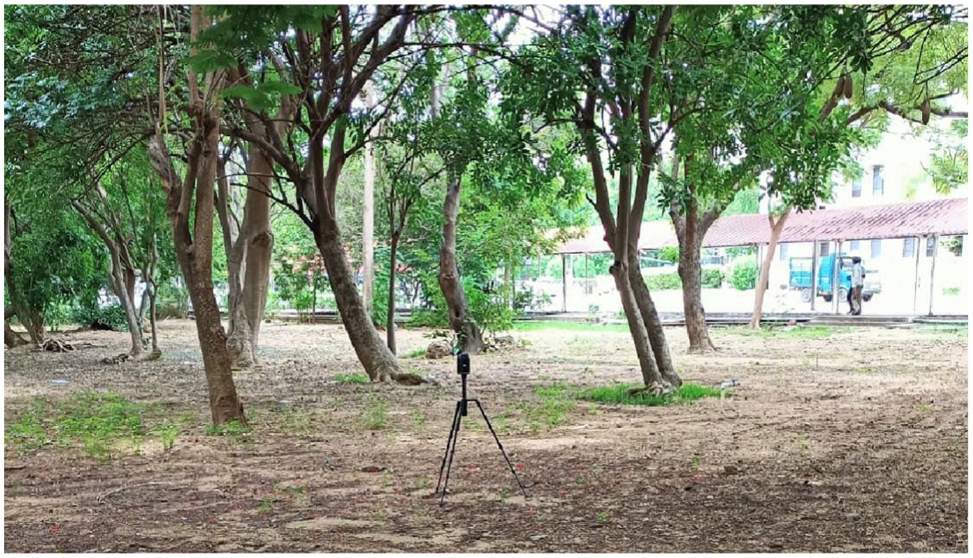
Figure 3. Sample photo showing the ground-based LiDAR survey of trees.

3 Results and discussion

The results and discussion section have been divided into three parts. The first part discusses the results of the histogram analysis followed by UGS extraction using different image classification methods. The results of UGS availability at city and ward levels using per capita and geographical area approaches are presented in Section 3.2. The results of UGS information at tree level using 3D LiDAR data are presented in Section 3.3.

3.1 Histogram analysis and UGS extraction

The plot of histograms for all the six classes is calculated using the R, G, and B values of representative areas (circular buffers in Figure 2), as shown in Figure 4. The histogram plots clearly show that the brightness values (0–255) of pixels in each band (R, G, and B) and their frequency distribution (count) are varying among the classes. It can be observed from Figure 4 that the UGS classes have mean pixel values (average of R, G, and B) in the range of 57–71, whereas the built-up, open land, and water bodies have mean values of 130, 180, and 23, respectively. This indicates that the UGS classes can easily be extracted from the GE image as they have distinct pixel values when compared with non-UGS classes such as built-up, open land, and water bodies. As shown in Figure 4, built-up land has pixels with values falling almost in the entire range of 0–255 (minimum 3 and maximum 255), and that is why the histogram is flat too. Open land has a very bright tone in the GE image of Figure 2, and that is why, it showed high pixel values (average pixel value of 180) when compared with histograms of other land cover classes (Figure 4). Water body, on the other hand, has very low pixel values in the range of 11–37 as it appeared dark in the GE image, as shown in Figure 2. Thus, the analysis of histograms revealed that the built-up, open land, and water bodies have distinct pixel values and counts, i.e., built-up has pixel values has spread throughout the range with very less pixel count; open land has high pixel values but with a count of less than 500; water bodies have low pixel values but with a very high count of 2,500. Thus, the pixel values and counts of non-UGS classes indicate that they can easily be differentiated when compared with UGS classes in the GE image and thus make the UGS extraction easier when image classification methods are applied on the GE image.

Figure 4

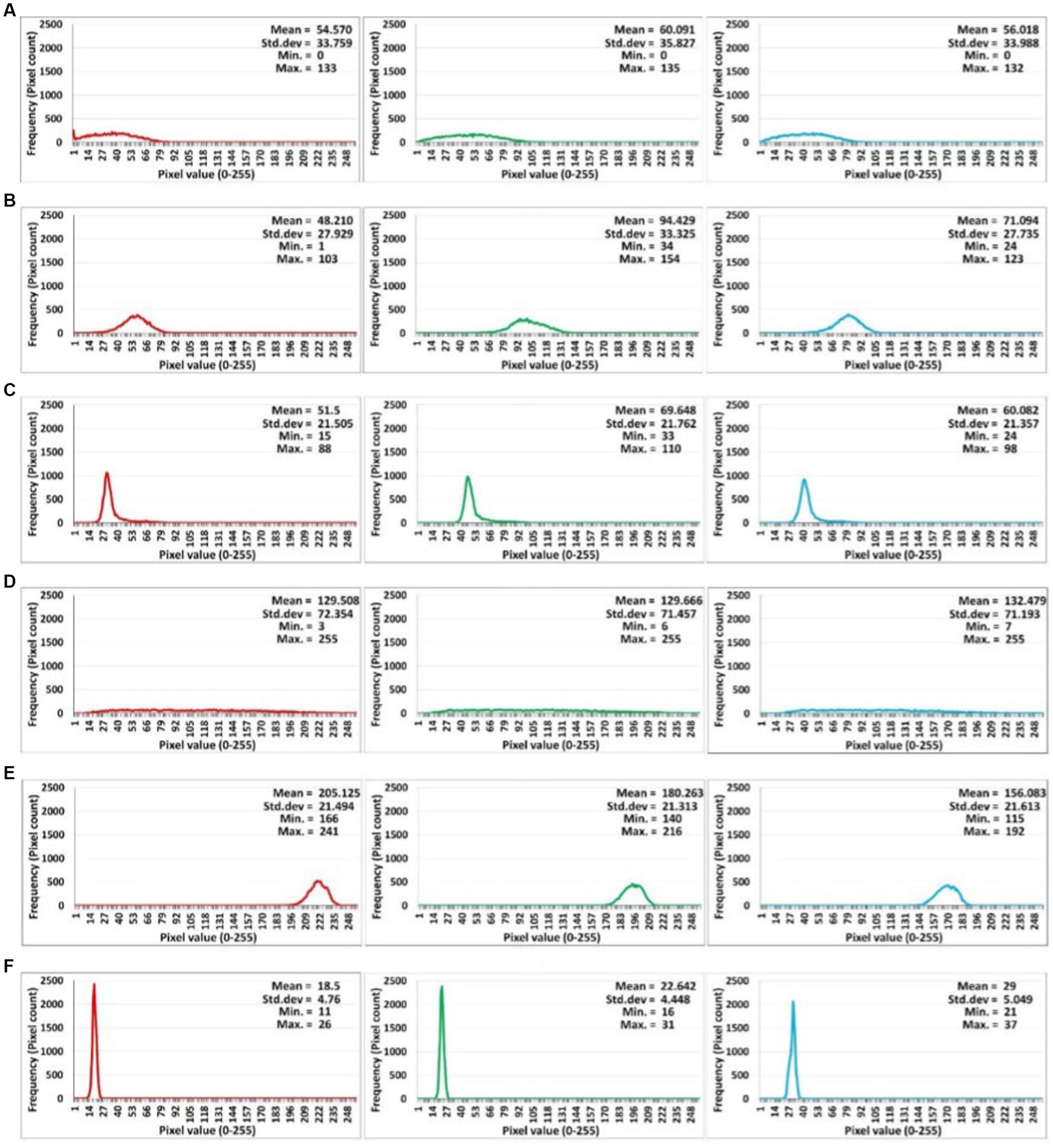
Figure 4. Plot of histograms for red band (left), green band (middle), and blue band (right) of the GE image for (A) tress, (B) shrubs/grassland, (C) cropland, (D) built-up, (E) open land, (F) waterbody.

Among the three UGS classes, the histograms differ in terms of pixel values and counts as shown in Figure 4. For example, trees have pixel counts less than 200, whereas shrubs and crop land have pixel counts of 400 and 1,000, respectively. The UGS histograms differ from each other in terms of shape also due to their varying pixel values. For example, trees are widespread (mean standard deviation of 35) and shrubs are medium-spread (mean standard deviation of 30), and crop lands are low-spread (mean standard deviation of 21). Though by visual observation, we can say that the histograms of all six classes are different, but it would be good if we do the relevant statistical test and confirm that the differences between the histograms are statistically significant. One of the popular tests for the histogram comparison called the “Kolmogorov–Smirnov (KS)” test was conducted using “Real Statistics” software (Zaiontz, 2023) in MS EXCEL. “One-Sample KS” test was used to find whether a sample comes from a population which has been normally distributed. The “Two-Sample KS” test was used to determine whether two samples come from the same population or not. As the objective was to check whether the histograms were significantly different from each other, the “Two-Sample KS” test was applied. The null hypothesis was that both samples come from a population with same distribution, and the alternate hypothesis was that they are not from the same population and do not have identical distributions. The test basically calculates the maximum distance between the cumulative distributions of two samples and then checks it with the critical value. If the test statistic is more than the critical value, the null hypothesis will be rejected, and alternate hypothesis will be accepted. In the present study, all the histograms shown in Figure 4 were compared with each other using the KS test, and the results are shown in Table 1. It can be seen that in all the cases, the test statistic is more than the critical value of 0.018, and thus, the null hypothesis can be rejected at 0.05 level of significance. Thus, the KS test confirms that the histograms in Figure 4 are not same, and the differences between them are statistically significant. Hence, it can be concluded that the GE image can be used for UGS extraction as pixel values of UGS classes differ from each other and also from other land cover classes. The maps of UGS for Vellore extracted using different classification methods are shown in Figure 5, and the corresponding accuracy assessment results are shown in Table 2. It can be observed from Table 2 that among all the methods, support vector machine (SVM) performed extremely well with an overall accuracy (OA) of 93% and Kappa coefficient of 0.881. Other methods such as maximum likelihood (ML), unsupervised, and object-based achieved only 69, 73, and 49%, respectively. In general, OA of more than 85% is considered to be the acceptable one. Based on this, it can be said that only SVM produced the acceptable results in extracting the UGS for Vellore using GE image. It is also evident from Figure 2 that on the south-western part of Vellore Corporation where the Bagayam reserved forest is located, it was correctly classified by the SVM method as trees and shrubs (Figure 5A) while the other methods could not (Figures 5B–D). The reason why SVM performed well is that it creates an optimal hyperplane from infinite number of decision boundaries by maximizing the distance between the classes and minimizing the misclassification errors. The reasons why other methods have not performed well were also analyzed. It can be observed from Table 2 (B, C) that 18 and 36 trees were misclassified as others by ML and ISODATA methods, respectively, and that is why the producer accuracy (PA) went low which finally resulted in less OA. Those misclassified trees were examined carefully in the GE image, and it was found that the shadow of the trees appeared black in color in the GE image (Figure 6A), and due to which, the ML and ISODATA classified it as water bodies (comes under “Others” category) rather than UGS. Similarly, the vice versa scenario also took place where the actual water bodies were misclassified as trees. For example, 15 and 12 accuracy assessment points actually fall in the “Others” category but were wrongly classified as trees by ML and ISODATA, respectively, as shown in Table 2 (B,C). The same can be observed in Figure 6B, where the presence of algae in a lake within our campus resulted in the water body to appear greenish in color in the GE image, and thus, it led to the misclassification as trees by ML and ISODATA, respectively.

Table 1

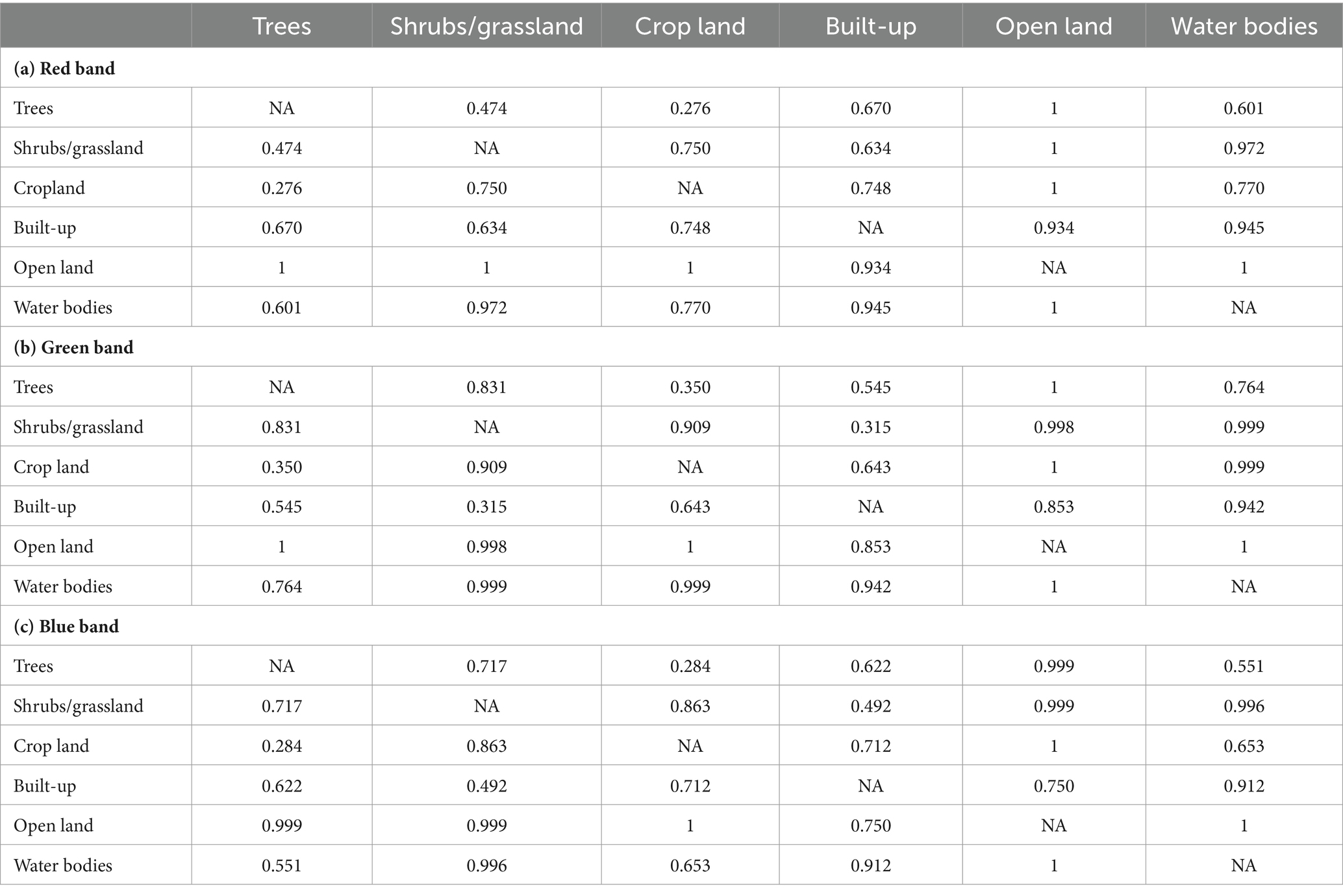
Table 1. Results of the Kolmogorov–Smirnov (KS) test.

Figure 5

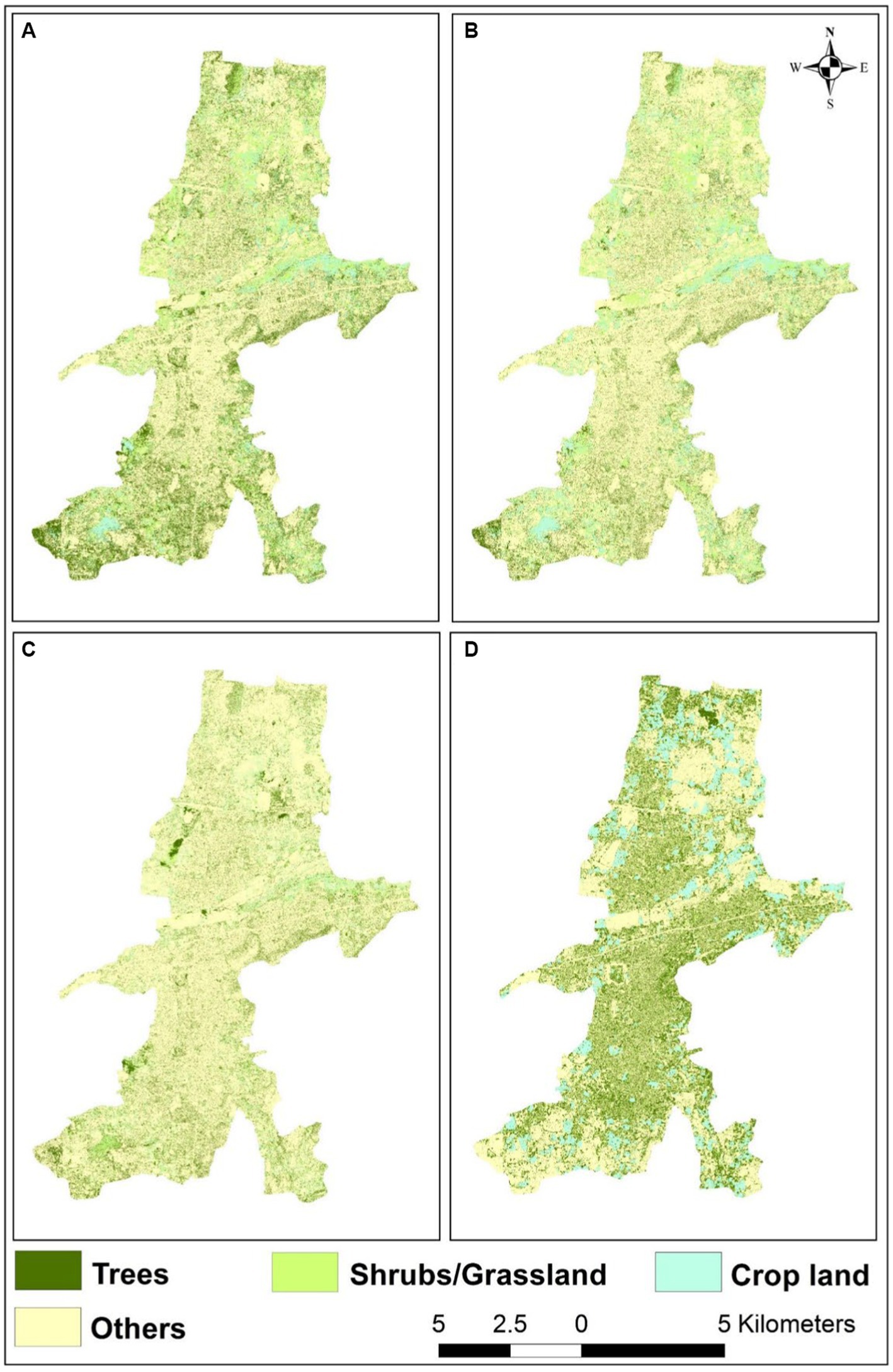
Figure 5. Maps showing UGS for Vellore extracted using (A) SVM, (B) maximum likelihood, (C) ISODATA, (D) object-based classification.

Table 2

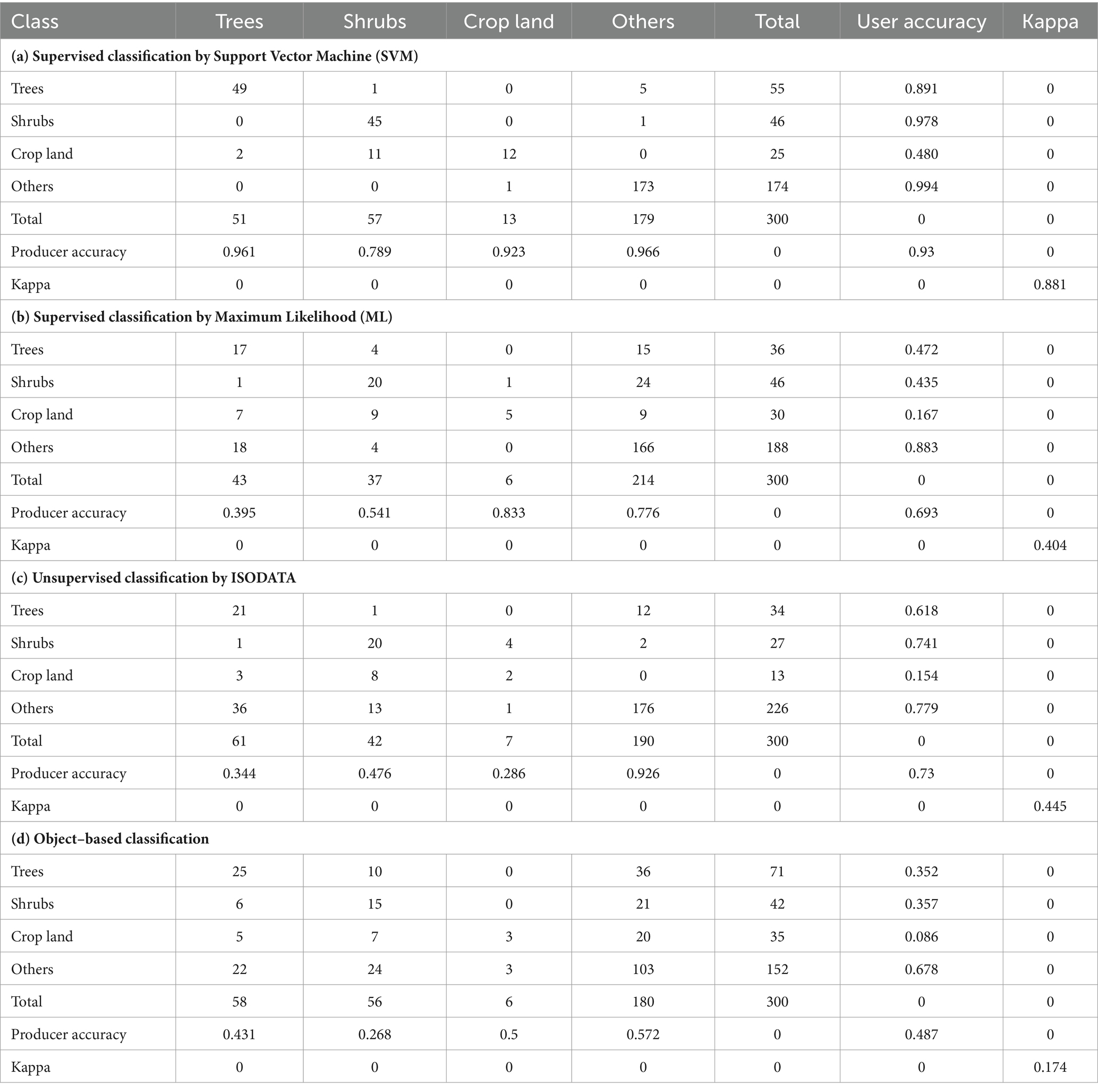
Table 2. Results of accuracy assessment.

Figure 6

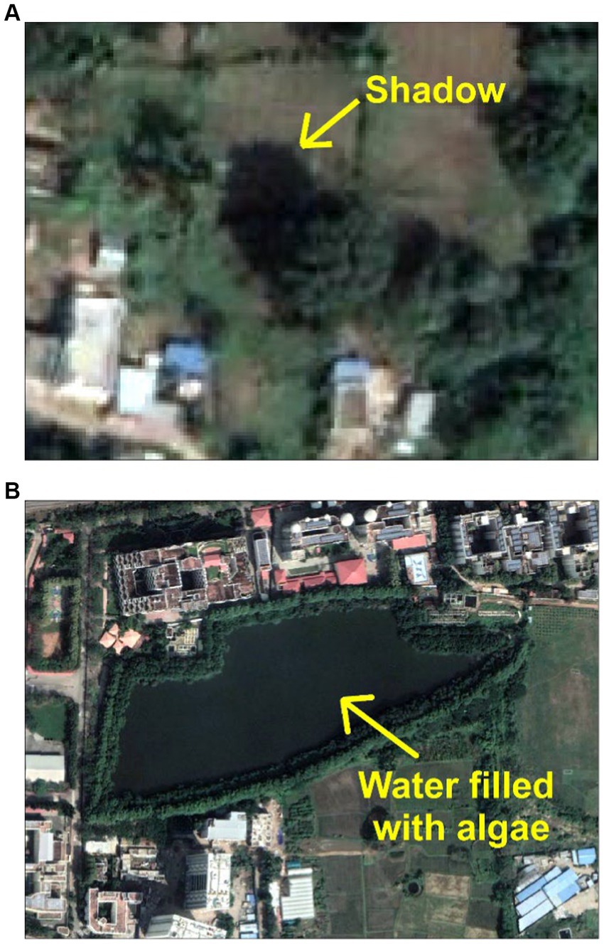
Figure 6. GE image showing (A) tree and its shadow (B) presence of algae in a lake.

In addition to the accuracy assessment, a field survey was also carried out to check whether SVM has correctly classified the UGS classes, namely, trees, shrubs/grassland, and crop land. Otteri Lake Park located in the south eastern part of Vellore was considered, and its GE image and the corresponding SVM output are shown in Figure 7. Three locations were identified for verification and are shown in Figure 7. The actual photos taken at those three locations are shown in Figure 8. There is a pedestrian footpath at location-1 with trees on both the sides, and this has been classified correctly by SVM as observed from Figure 7B (location-1). One of the branches of a tree was intersecting the footpath (Figure 8), which was captured by the SVM classification as shown in Figure 7B. In between the lake water and trees, shrubs were noticed in the field, which also was correctly classified by SVM, as shown in Figure 7B (location-1). This clearly indicates that the SVM performs well in differentiating the trees and shrubs in the GE image. To confirm this, one more location where only one single tree surrounded by shrubs was selected (location-2 of Figure 8), and it was found that the SVM correctly classified the tree and shrubs, as shown in Figure 7B location-2. The performance of SVM in classifying the crop land (location-3 of Figure 8) was also checked, and as expected, the SVM performed well in classifying the crop land, as shown in location-3 of Figure 7B. The coconut trees located on the upstream side of crop land was correctly classified as trees by SVM. Thus, the results of the field survey confirmed that SVM can be used to extract various UGS types in a GE image.

Figure 7

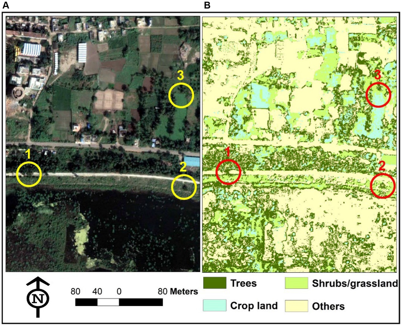
Figure 7. (A) GE image of Otteri Lake Park (B) SVM classified output of Otteri Lake Park.

Figure 8

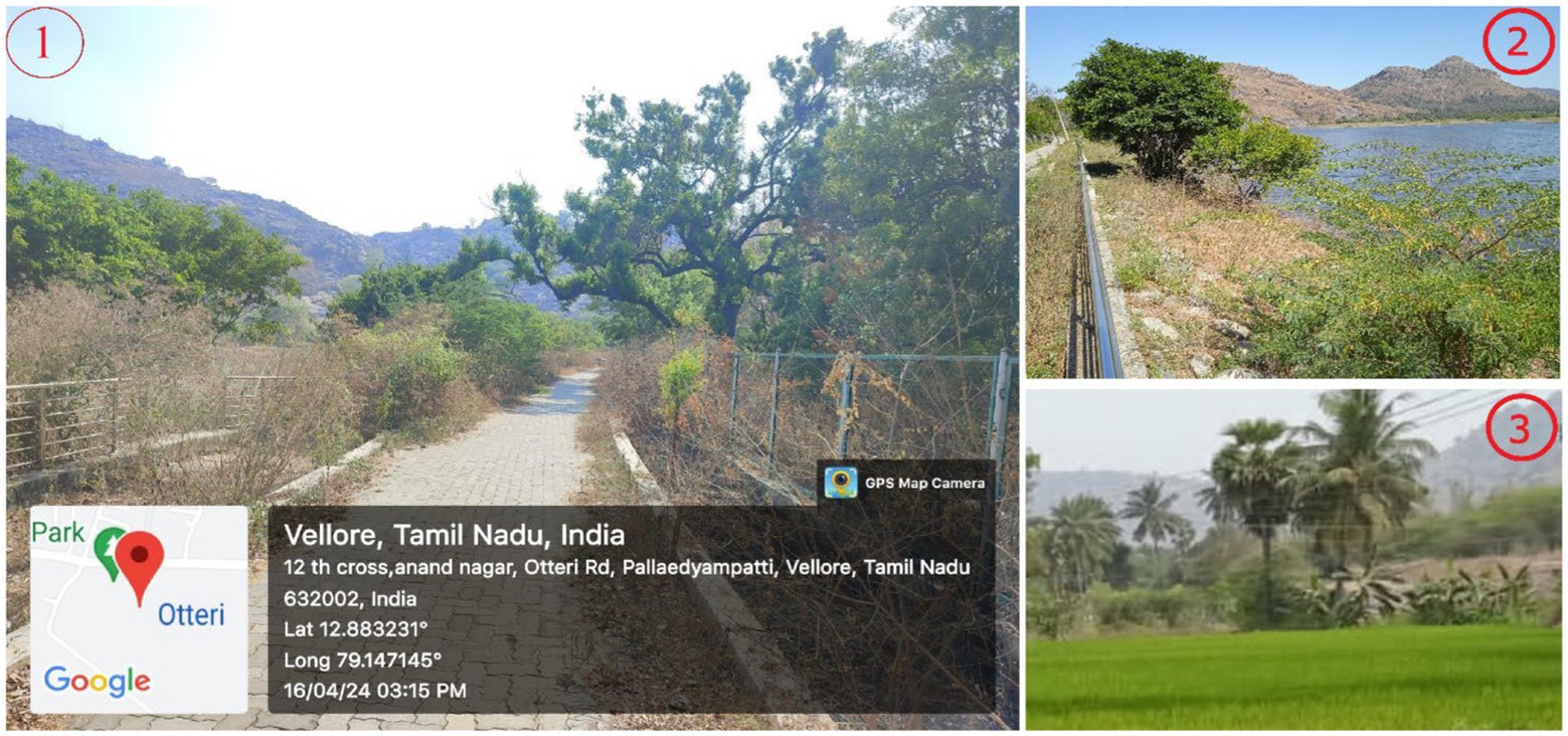
Figure 8. Actual photos taken at locations 1, 2, and 3 in Otteri Lake Park and its surroundings.

The results of UGS extraction discussed so far pertained to only the GE image covering Vellore city in Tamil Nadu. It would be better if we check whether SVM could perform well and produce similar results for other cities also. Hence, two wards numbered 28 and 36 measuring an area of 1.9 sq.km and 5.94 sq.km, respectively, in Warangal city of Telangana state in India were selected. The reason for taking these two wards is that in these wards, there is a mix of both UGS and various other classes such as built-up and water, as observed from the GE images shown in Figures 9A,B. The best performing SVM classification was applied, and the results are shown in Figures 9A,B. As the wards have been occupied majorly with educational institutions such as Kakatiya Medical College in ward 28 and National Institute of Technology in ward 36, crop land was absent, and only two UGS classes, namely, trees and shrubs/grassland were present. Accuracy assessment was carried out with 50 random points, and it was found that the OA was 98 and 91% for wards 28 and 36, respectively. It was evident from the classification results (Figures 9A,B) that SVM has correctly classified the UGS classes and “Others” when we compare the raw GE image and the classified output. Thus, the classification results clearly indicate that the GE image can be used to extract the green cover by using the SVM technique.

Figure 9

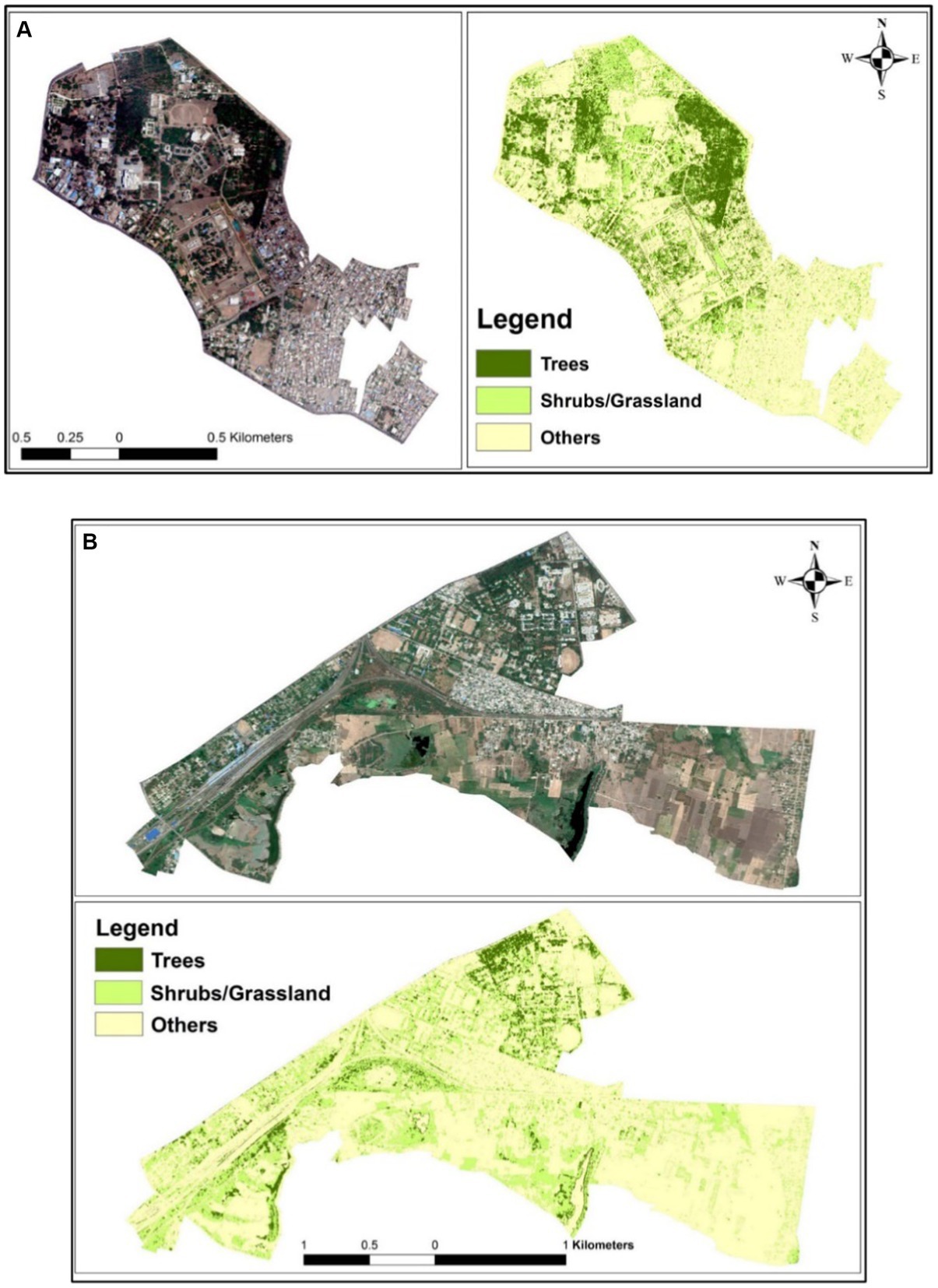
Figure 9. (A) GE image of ward 28 in Warangal, India (left), and the corresponding SVM classification output (right). (B) GE image of ward 36 in Warangal, India (left), and the corresponding SVM classification output (right).

3.2 Calculation of available UGS

Once the UGS map is prepared, the amount of available greenery based on per capita or geographical area can be calculated and checked against the standards. The present study carried out the same at ward level, and the results are shown in Figures 10A,B for per capita and percentage of geographical area, respectively. In India, the recommended UGS is 10–12 m² per person, and in terms of geographical area, it is recommended that 20–40% of the city’s geographical area should be covered by green (NITI Aayog, 2021; Roy and Fleischman, 2022). Hence, the per capita results in Figure 10A are shown in three categories, namely, <10m², 10–12 m², and >12 m²/person. Similarly in Figure 10B, the results are shown in three categories, i.e., <20, 20–40, and >40% of total area. The results revealed some interesting results regarding how the amount of greenery should be calculated in a city. For example, if the whole Vellore city in Figure 10 is considered, the percentage of UGS available is 42% [(UGS area (38.39 sq.km)/Total area (92.40 sq.km)) × 100], which is more than the recommended range of 20–40%. Similarly, if we consider the whole city, the available UGS per person is 97.84 m²/person [(UGS area (38.39 sq.km)/Population (392434)) × 1,000,000], which is far above the recommended 12 m²/person. However, if we do micro-level calculation, i.e., at the ward level as shown in Figures 10A,B, some of the wards (red colored) have not satisfied the criteria of per capita and/or percentage area, though the city as a whole has satisfied both the criteria. The red-colored wards numbered 28, 29, 32, 33, 34, 35, 38, and 55 which have not satisfied both the criteria are located in the old town of Vellore city, where one can observe mostly the commercial establishments and wholesale markets with dense built-up area without any green cover. This was the reason why those wards could not meet both the criteria though the city as a whole has satisfied. The results clearly indicate that the amount of greenery should be calculated at the micro or ward level rather than the macro or city level as the former gives more closer look into the surplus (green colored) and deficit (red colored) areas. The advantage of this ward-level analysis is that now the civic authorities can frame action plans to increase the greenery in red-colored wards so that all the 60 wards of the city can satisfy both the criteria of per capita and percentage area.

Figure 10

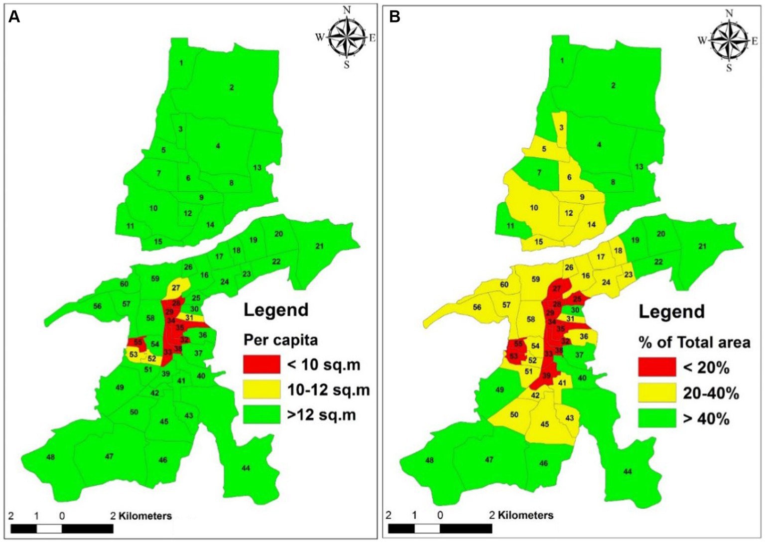
Figure 10. Ward-wise available greenery calculated through (A) Per capita approach (B) Percentage of total area approach.

3.3 UGS information at tree level using 3D LiDAR data

Though GE images can be used to extract UGS information, it is not possible to obtain individual tree level data such as height and diameter with GE. Hence, the present study used LiDAR data also to extract the individual trees in the campus, and the results are shown in Figure 11. The 3D models that are shown in Figure 11 were used to extract individual tree information such as height, diameter, and crown area, and the results are presented in Table 3. The height of trees was found to vary between 5 and 12 m, and the diameter varies from 0.1 to 0.7 m. The minimum and maximum crown areas of trees were measured as 19 and 164 sq.m, respectively. Such tree level information as observed in Table 3 is possible only with 3D LiDAR data. In addition, the tree health can be inferred using LiDAR data. For this, the Leaf Area Index (LAI) was calculated for each tree using the individual 3D model of trees extracted from the LiDAR data. LAI which is basically the ratio of the leaf area to the corresponding ground area is one of the major indicators of tree health and also helps to understand the green coverage of a tree. In general, the desert ecosystems would have LAI of less than 1, whereas the LAI can be as high as 9 for dense tropical forests (Campbell, 2023). In the present study, the LAI for the trees was found to vary from 2.094 to 8.2. This LAI is not a fixed one and is susceptible to seasonal changes. It will be highest during the spring season and may be lowest when leaves started shedding. Thus, with the help of LiDAR data, one can assess the tree health periodically based on whether the LAI is increasing or decreasing. The results of temperature in Table 3 reveal an interesting fact that when trees are nearby, the buildings and roads exhibit comparatively lesser temperature in the range of 31–34°C, whereas if trees are not there in the surrounding, buildings and roads exhibit higher temperature in the range of 34–44°C. Moreover, this highlights the need for having more green cover in cities which are covered with mostly of concrete structures that generally lead to high surface temperatures and strong heat islands. The main purpose of using LiDAR data is to show that if trees are adjacent to buildings or roads, it results in lesser heat islands when compared to the case where there are no trees.

Figure 11

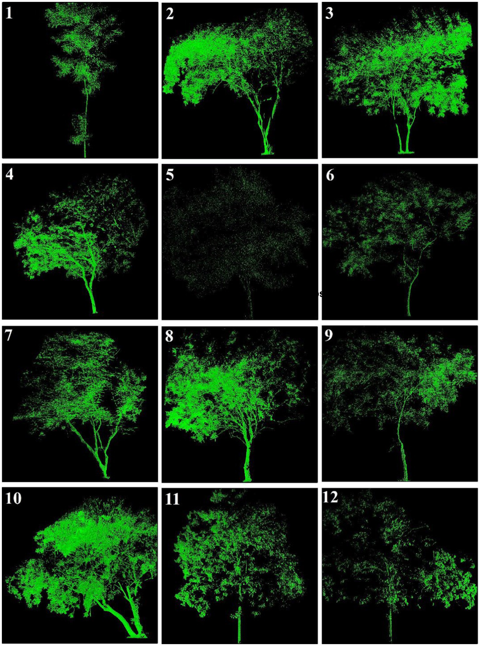
Figure 11. Individual 3D model of trees from LiDAR data. ¹Kakawate; ²Kigelia; ³Kigelia; ⁴Azadirachta indica; ⁵Bignonia; ⁶Azadirachta indica; ⁷Albizia Chinensis; ⁸Millingtonia hortensis; ⁹Albizia chinensis; ¹⁰Millettia pongamia/pinnata; ¹¹Tectona grandis; ¹²Tectona grandis.

Table 3

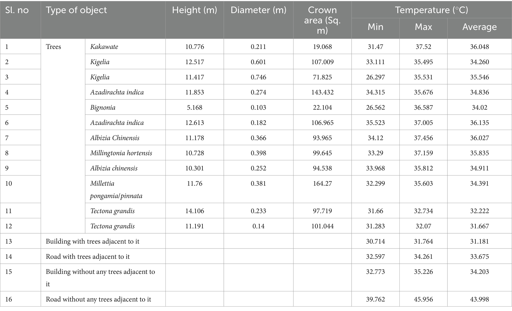
Table 3. Information about individual trees, buildings, and roads from LiDAR data.

4 Concluding remarks

Urbanization in developing countries such as India has resulted in the loss of precious green cover and demands the calculation of its extent periodically to check whether the city has sufficient green cover or not. As one can clearly observe the different types of green cover in GE images, the same can be utilized to obtain information on how much green space is actually available in a city or town. The present study attempted the same through histogram-based classification approach, where the histograms were analyzed first to check whether the green covers are spectrally differentiable when compared with other land covers, and then, various classification methods were applied to extract the green covered area from GE images. The results showed that SVM performed well with the highest accuracy in extracting green covered areas when compared with other methods. The extracted green cover was then used to check whether sufficient greenery was available or not at each ward of the city through per capita and percentage area methods. The results suggested that the existing practice of calculating the greenery by considering the city as a whole might not be sufficient as some wards do not meet the criteria. Moreover, the ward level analysis was found to be more suitable to identify the deficit and surplus areas. The LiDAR survey was also carried out, and the results showed the reduction in temperature due to the presence of green cover and thus highlighted the importance of green cover in a city in reducing the urban heat islands. The present study will be very useful to urban planners to map green cover from GE imagery, assess whether the city has sufficient quantity of green cover or not, calculate the loss in green cover due to urbanization and check whether green covered areas help in reducing the heat islands in a city.

Data availability statement

The original contributions presented in the study are included in the article/supplementary material, further inquiries can be directed to the corresponding author.

Author contributions

SG: Conceptualization, Data curation, Formal analysis, Investigation, Methodology, Visualization, Writing – original draft, Writing – review & editing. SK: Conceptualization, Methodology, Supervision, Validation, Visualization, Writing – original draft, Writing – review & editing.

Funding

The author(s) declare financial support was received for the research, authorship, and/or publication of this article. We would like to thank the management of Vellore Institute of Technology (VIT) for providing open access fund for publication of this article.

Conflict of interest

The authors declare that the research was conducted in the absence of any commercial or financial relationships that could be construed as a potential conflict of interest.

Publisher’s note

All claims expressed in this article are solely those of the authors and do not necessarily represent those of their affiliated organizations, or those of the publisher, the editors and the reviewers. Any product that may be evaluated in this article, or claim that may be made by its manufacturer, is not guaranteed or endorsed by the publisher.

References

Badiu, D. L., Ioja, C. I., Patroescu, M., Breuste, J., Artmann, M., Nita, M. R., et al. (2016). Is urban green space per capita a valuable target to achieve cities’ sustainability goals? Romania as a case study. Ecol. Indic. 70, 53–66. doi: 10.1016/j.ecolind.2016.05.044

Crossref Full Text | Google Scholar

Campbell, G. S. (2023). The researcher's complete guide to leaf area index (LAI). Meter, Washington. Available at: https://metergroup.com/education-guides/the-researchers-complete-guide-to-leaf-area-index-lai/.

Google Scholar

Congalton, R., and Green, K. (2019). Assessing the accuracy of remotely sensed data. 3rd Edn. Florida: CRC Press, Taylor & Francis Group.

Google Scholar

Datta, K., and Sarkar, S. (2019). Calculation of area, mapping and vulnerability assessment of a geomorphosite from GPS survey and high-resolution Google earth satellite image: a study in mama Bhagne Pahar, Dubrajpur C. D. Block, Birbhum district, West Bengal. Spat. Inf. Res. 27, 521–528. doi: 10.1007/s41324-019-00249-1

Crossref Full Text | Google Scholar

Elshayal, M. (2023). Elshayal smart GIS software for windows, ver. 21.02, Egypt.

Google Scholar

Emeterio, J. L. S., and Mering, C. (2021). Mapping of African urban settlements using Google earth images. Int. J. Remote Sens. 42, 4882–4897. doi: 10.1080/01431161.2021.1903613

Crossref Full Text | Google Scholar

ESRI (2023). Creating training samples. ArcGIS desktop help 10.6 spatial analyst extension. Environmental systems research institute (ESRI), USA.

Google Scholar

Farkas, J. Z., Hoyk, E., Morais, M. B., and Csomos, G. (2023). A systematic review of urban green space research over the last 30 years: a bibliometric analysis. Heliyon 9, e13406–e13414. doi: 10.1016/j.heliyon.2023.e13406

PubMed Abstract | Crossref Full Text | Google Scholar

Hwang, Y. H., Nasution, I. K., Amonkar, D., and Hahs, A. (2020). Urban Green space distribution related to land values in fast-growing megacities, Mumbai and Jakarta–unexploited opportunities to increase access to greenery for the poor. Sustain. For. 12, 1–17. doi: 10.3390/su12124982

Crossref Full Text | Google Scholar

Kefale, A., Fetene, A., and Desta, H. (2023). Users' preferences and perceptions towards urban green spaces in rapidly urbanized cities: the case of Debre Berhan and Debre Markos, Ethiopia. Heliyon 9, 1–16. doi: 10.1016/j.heliyon.2023.e15262

PubMed Abstract | Crossref Full Text | Google Scholar

Kowe, P., Mutanga, O., and Dube, T. (2021). Advancements in the remote sensing of landscape pattern of urban green spaces and vegetation fragmentation. Int. J. Remote Sens. 42, 3797–3832. doi: 10.1080/01431161.2021.1881185

Crossref Full Text | Google Scholar

Kuang, W., and Dou, Y. (2020). Investigating the patterns and dynamics of urban Green space in China’s 70 major cities using satellite remote sensing. Remote Sens. 12, 1–14. doi: 10.3390/rs12121929

Crossref Full Text | Google Scholar

Kumar, S., Wickramasooriya, A., and Dilini, S. (2022). Analysis of ammonium nitrate detonation destruction in Beirut city using geospatial techniques. Spat. Inf. Res. 30, 749–757. doi: 10.1007/s41324-022-00459-0

Crossref Full Text | Google Scholar

Kurekin, A. A., Miller, P. I., Avillanosa, A. L., and Sumeldan, J. D. C. (2022). Monitoring of coastal aquaculture sites in the Philippines through automated time series analysis of Sentinel-1 SAR images. Remote Sens. 14, 1–19. doi: 10.3390/rs14122862

Crossref Full Text | Google Scholar

Lahoti, S., Kefi, M., Lahoti, A., and Saito, O. (2019). Mapping methodology of public urban green spaces using GIS: an example of Nagpur city, India. Sustainability 11, 1–23. doi: 10.3390/su11072166

Crossref Full Text | Google Scholar

Li, W., Dai, F., Diehl, A. J., Chen, M., and Bai, J. (2023). Exploring the spatial pattern of community urban green spaces and COVID-19 risk in Wuhan based on a random forest model. Heliyon 9, e19773–e19712. doi: 10.1016/j.heliyon.2023.e19773

PubMed Abstract | Crossref Full Text | Google Scholar

Li, H., Han, Y., and Chen, J. (2020). Combination of Google earth imagery and Sentinel-2 data for mangrove species mapping. J. Appl. Remote. Sens. 14:010501. doi: 10.1117/1.JRS.14.010501

Crossref Full Text | Google Scholar

Li, L., Xu, C., Xu, X., Zhang, Z., and Cheng, J. (2022). Inventory and distribution characteristics of large-scale landslides in Baoji City, Shaanxi Province, China. ISPRS Int. J. Geo Inf. 11, 1–21. doi: 10.3390/ijgi11010010

Crossref Full Text | Google Scholar

Lind, E., Prade, T., Sjöman, D. J., Levinsson, A., and Sjöman, H. (2023). How green is an urban tree? The impact of species selection in reducing the carbon footprint of park trees in Swedish cities. Front. Sustain. Cities 5:1182408. doi: 10.3389/frsc.2023.1182408

Crossref Full Text | Google Scholar

Markovic, M., Cheema, J., Teofilovic, A., Epic, S., Popovic, Z., Dubljevi, J. T., et al. (2021). Monitoring of spatiotemporal change of Green spaces in relation to the land surface temperature: a case study of Belgrade, Serbia. Remote Sens. 13, 1–21. doi: 10.3390/rs13193846

Crossref Full Text | Google Scholar

MoHFW (2020). Report of the technical group on population projections. New Delhi: National commission on population, Ministry of Health & family welfare (MoHFW).

Google Scholar

NITI Aayog (2021). Urban transformation sector report, development monitoring and evaluation office. NITI Aayog, Government of India.

Google Scholar

Pouya, S., and Majid, A. (2022). Evaluation of urban green space per capita with new remote sensing and geographic information system techniques and the importance of urban green space during the COVID-19 pandemic. Environ. Monit. Assess. 194, 633–619. doi: 10.1007/s10661-022-10298-z

PubMed Abstract | Crossref Full Text | Google Scholar

Ramaiah, M., and Avtar, R. (2019). Urban green spaces and their need in cities of rapidly urbanizing India: a review. Urban Sci. 3, 1–16. doi: 10.3390/urbansci3030094

Crossref Full Text | Google Scholar

Rehman, Z., Zubair, M., Hafiz, D. O., and Manzoor, S. A. (2024). Biodiversity and quality of urban green landscape affect mental restorativeness of residents in Multan, Pakistan. Front. Sustain. Cities 5:1286125. doi: 10.3389/frsc.2023.1286125

Crossref Full Text | Google Scholar

Roy, A., and Fleischman, F. (2022). The evolution of forest restoration in India: the journey from precolonial to India's 75th year of Independence. Land Degrad. Dev. 33, 1–14. doi: 10.1002/ldr.4258

Crossref Full Text | Google Scholar

Sathyakumar, V., Ramsankaran, R., and Bardhan, R. (2020). Geospatial approach for assessing spatiotemporal dynamics of urban green space distribution among neighbourhoods: a demonstration in Mumbai. Urban For. Urban Green. 48, 126585–126516. doi: 10.1016/j.ufug.2020.126585

Crossref Full Text | Google Scholar

Semeraro, T., Scarano, A., Buccolieri, R., Santino, A., and Aarrevaara, E. (2021). Planning of urban Green spaces: an ecological perspective on human benefits. Land 10, 1–25. doi: 10.3390/land10020105

Crossref Full Text | Google Scholar

Shekhar, S., and Aryal, J. (2019). Role of geospatial technology in understanding urban green space of Kalaburagi city for sustainable planning. Urban For. Urban Green. 46, 126450–126412. doi: 10.1016/j.ufug.2019.126450

Crossref Full Text | Google Scholar

Sun, P., Song, Y., and Lu, W. (2022). Effect of urban Green space in the hilly environment on physical activity and health outcomes: mediation analysis on multiple greenery measures. Land 11, 1–19. doi: 10.3390/land11050612

Crossref Full Text | Google Scholar

Sun, X., Tan, X., Chen, K., Song, S., Zhu, X., and Hou, D. (2020). Quantifying landscape-metrics impacts on urban green-spaces and water-bodies cooling effect: the study of Nanjing, China. Urban For. Urban Green. 55, 126838–126811. doi: 10.1016/j.ufug.2020.126838

Crossref Full Text | Google Scholar

Zaiontz, C. (2023). Real statistics using Excel. Available at: https://www.real-statistics.com/free-download/ (Accessed December 24, 2023).

Google Scholar