Effects of Spatial Resolution on Burned Forest Classification With ICESat-2 Photon Counting Data

Introduction

Forests store a huge amount of carbon and play a critical role in controlling global carbon balancing and cycling (Rödig et al., 2019). However, increased frequency and extent of fires are a growing concern (Balch et al., 2017; Cattau et al., 2020; Liu and Yang, 2020) and threaten the sustainability of terrestrial ecosystems. Fires have become more severe and destructive in response to a warming climate (Schoennagel et al., 2017), with many examples such as the 2018 California wildfire, the 2019 Amazon forest fire, and the 2020 Australia wildfire. These extreme fire events emphasize the necessity of fire occurrence monitoring and forecasting over space and time (Fusco et al., 2019). Classifying burned forests is crucial to forest dynamics monitoring and fire risk analysis (Hawbaker et al., 2020). Burned forest data are also employed for the estimation of terrestrial ecosystems responses to climate change (Aragão et al., 2018), and the projection of future climate. Accurately classifying burned forests serves as a basis for the analysis of monitoring carbon emissions and understanding the effects of climate change on ecosystems.

Remotely sensed data have been adopted for regional or global burned forest classification for decades (Chuvieco et al., 2019). Fire-induced changes such as vegetation removal, canopy thinning, and charcoal deposition, cause spectral shifts, which favor the application of multispectral remote sensing images. Spectral indices like differenced Normalized Burn Ratio (dNBR) index (Fraser et al., 2017), classification methods like Random Forest (Gibson et al., 2020), and time-series analysis method (Roteta et al., 2019) are commonly used in fire monitoring. However, optical images are limited in capturing three-dimensional (3D) vegetation structures, which makes it difficult to obtain under canopy fire information and canopy height measurements. Light detection and ranging (LiDAR) offers an opportunity to provide 3D canopy structures, which is an essential complement to existing image-based approaches in burned area mapping (Liu et al., 2020). Airborne LiDAR has been applied for classifying fire severity and forest fuel types with good accuracy (Wang and Glenn, 2009; Montealegre et al., 2014). Wang and Glenn (2009) mapped fire severity at 5 m spatial resolution based on height differences of pre- and post-fire airborne LiDAR data with an overall accuracy of 84%. Montealegre et al. (2014) employed a logistic regression model to classify forest fires at 25 m spatial resolution based on post-fire airborne LiDAR data, producing an accuracy of up to 85.5%. Garcia et al. (2017) integrated post-fire airborne LiDAR data and Landsat images to estimate consumed biomass at 30 m spatial resolution. Fernandez-Manso et al. (2019) combined Hyperion data and airborne LiDAR data to analyze burn severity in Mediterranean forests at 30 m spatial resolution. Although airborne LiDAR captures detailed vegetation structures with high accuracy, the application over large areas is constrained due to high expenses and large data volumes associated with data acquisition and processing.

Spaceborne LiDAR is instrumental for global monitoring with fixed footprint and revisit time (Popescu et al., 2018; Neuenschwander and Pitts, 2019), providing large coverage and repeatable observations. National Aeronautics and Space Administration’s (NASA) first Ice, Cloud, and land Elevation Satellite (ICESat) mission, which carried the Geoscience Laser Altimeter System (GLAS), launched in January 2003 and stopped operation in October 2009. The footprint and the sampling distance of GLAS beams were 65 and 170 m, respectively, with a wavelength of 1,064 nm (Zwally et al., 2002). GLAS recorded backscattered energy with a full-waveform measurement for each footprint. The waveform data were used to evaluate fire disturbance in Alaska forests (Goetz et al., 2010). Moreover, García et al. (2012) used GLAS data to characterize canopy fuels in southern forests in the United States. However, the footprint of ICESat is coarse and the samples are sparse, which limit the acquisition of finer 3D details. NASA’s Global Ecosystem Dynamics Investigation (GEDI), a current full-waveform lidar mission, provides significant improvements in the footprint size (25 m) and the sampling distance (60 m) at a wavelength of 1,064 nm (Duncanson et al., 2020). However, GEDI only collects data between 51.6° North and 51.6° South, which limits its application to ecoregions in higher latitudes.

NASA’s Ice Cloud and land Elevation Satellite-2 (ICESat-2) mission, launched in September 2018 with the Advanced Topographic Laser Altimeter System (ATLAS) (Leigh et al., 2015), is a promising solution to the drawbacks of the initial ICESat mission. ATLAS, a photon counting LiDAR with a 14 m footprint and the along track sampling distance of 0.7 m, is sensitive to a single photon level (Popescu et al., 2018). ATLAS emits three pairs of beams with a wavelength of 532 nm. Each pair contains a strong beam and a weak beam distinguished by a designed energy ratio of 4:1. The ICESat-2 mission provides datasets like the geolocated photon data (ATL03), which comprises precise latitude, longitude and elevation of each photon point where a photon interacts with land surface. Some photon filtering algorithms like an adaptive ground and canopy height retrieval algorithm (Popescu et al., 2018) and ICESat-2 land and vegetation product algorithm (Neuenschwander and Pitts, 2019) were created to remove noise and retrieve ground and canopy photon points in ATL03. Neuenschwander and Pitts (2019) produced the Land and Vegetation height product (ATL08) based on the classified ATL03 photon points. The ATL08 product, with a nominal spatial resolution of 100 m by 14 m, provides various canopy and terrain related metrics in each segment such as mean canopy height, max canopy height, canopy openness, and the number of canopy points. Liu et al. (2020) leveraged ATL08 data to classify burned forests along ICESat-2 ground tracks with an overall accuracy of up to 83%. Information on the vertical structure of burned and unburned segments is useful for scaling up canopy characteristics related to fire damage, fire risk, and fire-caused carbon emissions.

Previous studies were focused on a specific spatial resolution when using LiDAR data in fire analysis, e.g., 5, 30, and 100 m. However, it must be noticed that spatial resolution has significant impacts on land cover classification (Roth et al., 2015) and canopy structure characterization (Gwenzi et al., 2016). Reese et al. (2002) estimated forest parameters like wood volume with Landsat data and found that the accuracy was better over larger areas (e.g., 19 hectares) than at the pixel level. Moreover, the relationship between spectral data and leaf area index was better based on Moderate Resolution Imaging Spectroradiometer (MODIS) data than using Landsat data (Cohen et al., 2003). Roth et al. (2015) classified species distribution with Airborne Visible/Infrared Imaging Spectrometer (AVIRIS) data at 20, 40, and 60 m spatial resolutions, concluding that coarser spatial resolution contributes to higher accuracy. Gwenzi et al. (2016) compared the accuracies of 14, 25, and 50 m segment lengths when using simulated ICESat-2 photon counting data to depict canopy height, highlighting that 25 m is a good choice. Yet, few studies have fully investigated the effects of spatial resolution when classifying burned forests with LiDAR data.

In this study, we sought to analyze the effects of spatial resolution on burned forest classification based on ICESat-2 photon counting data. ATL03 data from typical forests, the temperate forest in California and the boreal forest in Alberta, were filtered by two algorithms, the adaptive ground and canopy height retrieval algorithm (hereafter, AGCH) and the ICESat-2 land and vegetation product algorithm (hereafter, ILV). Twenty-six canopy related metrics were calculated based on filtered photon points at different spatial resolutions, i.e. 10, 30, 60, 100, 200, and 250 m. The Random Forest method was leveraged to classify burned forests along ICESat-2 ground tracks. Sentinel-2 images-derived landcover maps were adopted to avoid interference of different land cover types. The main goal was to investigate the effects of spatial resolution on burned forest classification using LiDAR data. Our specific objectives were: 1) to analyze the scale effects of LiDAR data on canopy characterization 2) to compare the accuracies of burned forest classification with ICESat-2 data at different spatial resolutions; 3) to compare the differences between strong beams and weak beams in burned forest classification.

Materials and Method

Study Sites

Two study areas (Figure 1), the temperate forest in northern California, United States, and the boreal forest in Alberta, Canada, were employed to compare canopy structures of different forest ecosystems and the influence of fire disturbances. For the temperate forest in northern California, two major fire events occurred over the study site (Figure 2). The Carr Fire happened west of Shasta Lake, starting on July 23, 2018, and was contained on August 30, 2018. The Delta Fire started on September 5, 2018, and stopped on October 7, 2018, in Shasta-Trinity National Forest. The elevation of this region ranges from 500 to 1,600 m. The whole region is dominated by species including gray pine (Pinus sabiniana), ponderosa pine (Pinus ponderosa), blue oak (Quercus douglasii), canyon live oak (Quercus chrysolepis), and Douglas-fir (Pseudotsuga menziesii) with scattered shrubs, grasslands, and bare grounds (Liu et al., 2020).

FIGURE 1

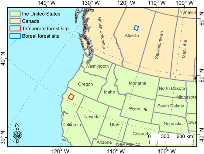
FIGURE 1. Locations of two study areas: the temperate forest in northern California, United States, and the boreal forest in Alberta, Canada.

FIGURE 2

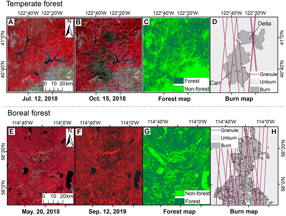
FIGURE 2. Sentinel-2 data for both study sites: (A) pre-fire image, (B) post-fire image, (C) forest map and (D) burn map in the temperate forest, California; (E) pre-fire image, (F) post-fire image, (G) forest map and (H) burn map in the boreal forest, Alberta. All images were displayed in a false-color composite (Near Infrared-Red-Green). The black boundaries of burned regions in burn maps were fire perimeters.

For the boreal forest in Alberta, Canada (Figure 2), a large wildfire happened in the Slave Lake district on May 13, 2019, and formed a fire complex. After burning for about 60,000 hectares, this fire was contained in late June 2019. The elevation of this region ranges from 400 to 800 m. Dominant species are black spruce (Picea mariana), white spruce (Picea glauca), balsam fir (Abies balsamea), lodgepole pine (Pinus contorta), and jack pine (Pinus banksiana) with a few shrubs like sheep-laurel (Kalmia angustifolia) and Labrador tea (Rhododendron groenlandicum). Due to high latitudes, boreal forests tend to have long winter seasons and short growing seasons.

Data

ICESat-2/ATLAS Data

ATL03 data provide accurate geolocation (x, y, z) of each photon point where a photon interacts with the land surface. However, due to the fact that ATLAS emits green beams (532 nm), there are many solar background noises in ATL03 (Neuenschwander and Pitts, 2019) and signals will often be obstructed by clouds. ATL03 data are distributed in hdf5 format with an average file size of 3–4 GB per granule. In this study, the ATL03 data whose ground track went through the burned areas were downloaded from the National Snow & Ice Data Center (NSIDC). For the temperate forest in California, ATL03 data acquired from April to December, which were close to the fire time (July to October), in both 2018 and 2019 after the fire events were downloaded. As for the boreal forest in Alberta, ATL03 data within April and October, which were close to the fire time (May to June), in both 2019 and 2020 after the fire event were obtained. There were twelve granules and nineteen granules for the temperate forest fire and the boreal forest fire (Figures 2D,H; Supplementary Table S1), respectively. ATL08 data corresponding to the selected ATL03 products were also downloaded for further analysis. In ATL08, the cloudy and empty segments were filled with a huge value, 3.4028 × 10³⁸, which were removed in this study to avoid cloud interference.

Reference Maps

Sentinel-2 Multi-Spectral Instrument (MSI) data were used to produce reference landcover maps since 10 m spatial resolution provides more details than ICESat-2/ATLAS’s 14 m footprint. Sentinel-2 images were atmospherically corrected with the Sen2Cor tool. In this study, only bands two to four, band 8, and bands 11–12 of Senitnel-2 data were employed, where the bands 11–12 were resampled to 10 m. For the temperate forest in California, pre- and post-fire Sentinel-2 images were obtained on July 12, 2018, and October 15, 2018 (Figure 2), respectively. For the boreal forest site, a pre-fire image was acquired on May 20, 2018, since there were no clear images before the fire event in 2019. Post-fire images were acquired on September 12, 2019. For each study area, the Iterative Self-Organizing Data Analysis Technique (IsoData) was employed to classify the pre-fire Sentinel-2 image into 20 classes in ENVI 5.5 (Harris Geospatial Solutions). Based on Google Maps and visual interpretations, the 20 classes were merged into forest and non-forest types. 200 randomly selected samples, 100 for forest and 100 for non-forest, were created to assess classification accuracy. The confusion matrix was established based on the visual interpretation of Google Maps and Sentinel-2 images for each sample. Overall accuracy (OA) and kappa of the forest map in the temperate forest in California were 87% and 0.74, respectively. As for the boreal forest, OA and kappa were 87.5% and 0.75, respectively. In the temperate forest of northern California, the fire perimeters were downloaded from the CalFire (https://frap.fire.ca.gov/mapping/gis-data/). For the boreal forest in Alberta, fire perimeters were downloaded from the Alberta Wildfire (https://wildfire.alberta.ca/resources/historical-data/spatial-wildfire-data.aspx). These fire perimeters were rasterized to 10 m spatial resolution to produce fire masks (or so-called burn maps) (Figures 2D,H). 200 randomly created samples, 100 for the burned region and 100 for the unburned region, were used to establish a confusion matrix for each burn mask. Based on interpretations of pre- and post-fire Sentinel-2 images as well as Google Maps, OA and kappa of the burn map in the temperate forest were 82.5% and 0.65 (Supplementary Table S2), respectively. For the boreal forest in Alberta, OA was 84% and kappa was 0.68 (Supplementary Table S3).

Filtering ATL03 Data

Two typical photon filtering/classification algorithms, the adaptive ground and canopy height retrieval algorithm (AGCH) (Popescu et al., 2018) and the ICESat-2 land and vegetation product algorithm (ILV) (Neuenschwander and Pitts, 2019), were adopted to remove noise points and classify ground and canopy points (Figure 3). We used filtered results from the two algorithms to avoid potential biases from a single method. For the AGCH method, ATL03 data were filtered following the procedures in Popescu et al. (2018). In the ILV method, labels (noise, ground, or canopy) of signal photon points in ATL03 were recorded in the corresponding ATL08 product based on the Data Product Algorithm Theoretical Basis Document (ATBD). Therefore, we read those labels from ATL08 to match ATL03 (Supplementary Figure S1).

FIGURE 3

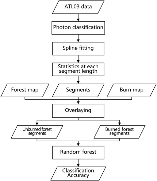
FIGURE 3. Flow chart for the analysis of scale effects on burned forest classification with ICESat-2 LiDAR data.

Ground surfaces were derived by fitting smooth splines in R (version 3.5.1) with the classified ground points. Subtracting the ground surface from point elevations, we got actual canopy height (also called relative height). To compare the effects of spatial resolutions, canopy heights were summarized within fixed segment length, i.e., 10, 30, 60, 100, 200, and 250 m. These segment lengths were chosen based on popular spatial resolutions of remote sensing data. For instance, 10, 30, and 60 m refer to Sentinel-2 and Landsat data. Moreover, 60 m is close to the footprint of ICESat/GLAS (65 m). 100 m is the original segment length of the ATL08 product. As for 200 m, it is double of ATL08 segment length which illustrates the effects of merging two 100 m segments. 250 m is a spatial resolution of MODIS data. Twenty-six canopy related metrics (Table 1) were derived based on the filtered ATL03 points and corresponding relative canopy height in each segment. In this study, both weak beams and strong beams were filtered and employed in further comparisons.

TABLE 1

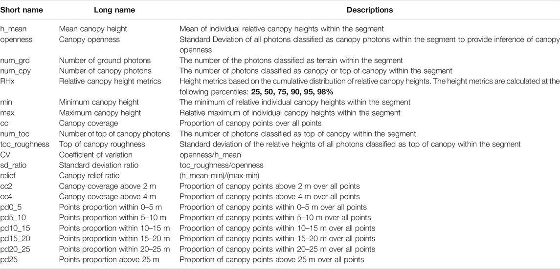
TABLE 1. Twenty-six canopy related metrics and their definitions.

To figure out which metrics are changing significantly along with spatial resolutions, a non-parametric method, the Kruskal-Wallis rank sum test, was employed in R. The Kruskal-Wallis test is a rank-based method that is often employed to determine whether there are statistically significant differences among different groups. When the test result is significant (p < 0.05), we can further use multiple comparisons to figure out which groups are significantly different. The non-parametric multiple comparisons in the “npmc” package in R was adopted in this study to further investigate whether the differences of any two groups are significant. On the other hand, when the Kruskal-Wallis test is not significant (p > 0.05), the values in different groups can be regarded as close and comparable.

Classifying Burned Forest

The Random Forest classification method was employed in this study to classify burned segments of ICESat-2 data from unburned ones. We chose the Random Forest method because it has no assumptions on data distributions (non-parametric) and can process high-dimensional data (Maxwell et al., 2018). Moreover, the Random Forest method doesn’t require extra testing samples since the model is generalized using a bootstrap procedure (Breiman, 2001). Each segment was overlaid with the corresponding forest map first to select forest segments (Figure 4). If over 90% of pixels within a segment were forest (in this study, a pixel was counted even though only part of it is within the segment), this segment would be defined as a forest segment. In the same way, the forest segments were overlaid with the corresponding burn map. If over 90% of pixels within a forest segment were burned, this forest segment would be defined as a burned forest segment. Conversely, if over 90% of pixels were unburned, this forest segment would be labeled as an unburned forest segment.

FIGURE 4

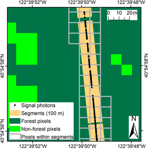
FIGURE 4. Overlaying segments with reference maps (forest map or burn map) to select training datasets, where the segments were 100 m in length and 14 m in width. The same routine works for segments with 10, 30, 60, 200, and 250 m length.

Due to the existence of outliers in canopy metrics, a range of µ ± 2σ was employed to exclude extreme values in each metric, where µ is the average and σ is the SD. For a specific metric, the average value (µ) and the SD (σ) of forest segments were calculated and those forest segments whose values were beyond the range of (µ−2σ, µ+2σ) were regarded as outliers and removed. After removing outliers, there were 3,683 and 6,518 (Supplementary Table S4) 100 m forest segments left in the temperate forest and the boreal forest, respectively, based on the AGCH filtering algorithm using strong beams. Twenty-six canopy metrics of each segment were input into the Random Forest model with a corresponding label: 0-unburned, 1-burned. Samples in the temperate forest were used for training in the R package “randomForest” with 1,000 trees. The best number of splits, which means the best number of predictors in a bootstrap step, was determined by a minimum out of bag (OOB) error. In this study, the minimum OOB error was adopted to calculate classification accuracy (overall accuracy = 1-OOB error). The same routine was employed to train another Random Forest model for the boreal forest. We didn’t combine samples from the temperate forest and the boreal forest to produce a single Random Forest model because we wanted to get the best classification accuracy for each forest type but not an average accuracy. Moreover, the temperate forest and the boreal forest have significantly different canopy structures (Figures 5, 6, 8) which favor separate models.

FIGURE 5

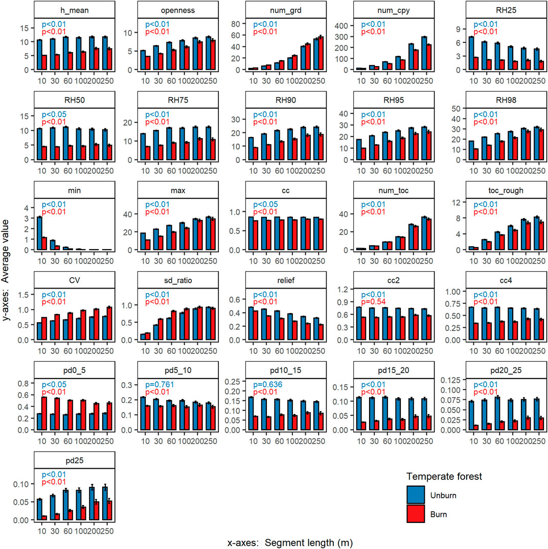
FIGURE 5. The average value of each canopy related metric in the temperate forest in California based on the AGCH algorithm using strong beams, where the error bars are standard errors. P values are the significance of the Kruskal-Wallis test.

FIGURE 6

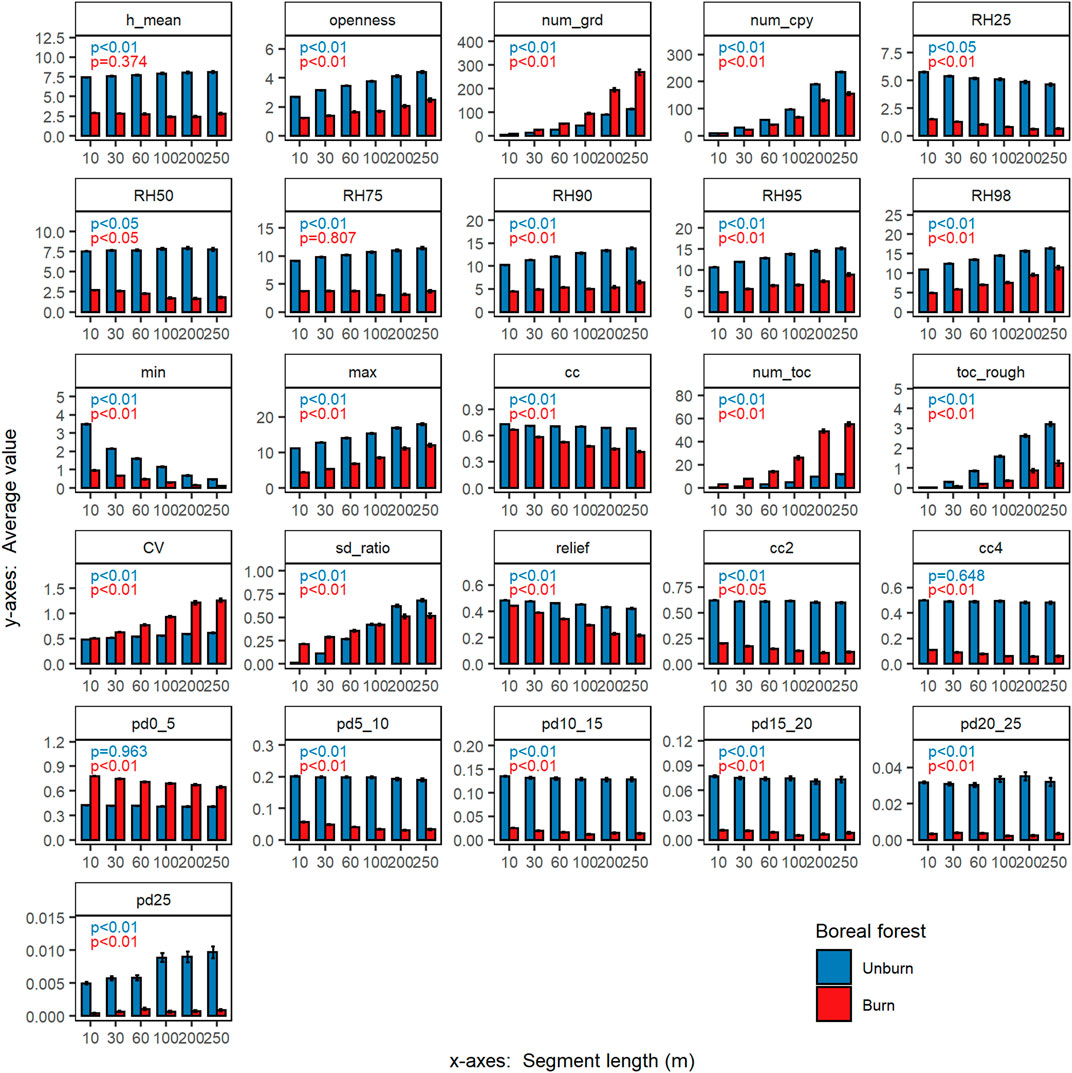
FIGURE 6. The average value of each canopy related metric in the boreal forest in Alberta based on the AGCH algorithm using strong beams, where the error bars are standard errors. P values are the significance of the Kruskal-Wallis test.

Results

Canopy Structures at Different Scales

Average values of canopy metrics are changing along with spatial resolutions in both burned and unburned samples (Figure 5), which means spatial resolutions can influence canopy structures we detected. Moreover, spatial resolution impacts measurements in both the temperate forest (Figure 5) and the boreal forest (Figure 6). Burned samples have lower numbers of canopy photons than the unburned ones, which is due to biomass consumption and sparser canopy after the fire. For the maximum canopy height (max), the values are also increasing when spatial resolutions get coarser, which is because high points are averaged by those low points when spatial resolutions are finer (10 or 30 m). Similar patterns were found in samples produced by the ILV algorithm (Supplementary Figures S2, S3).

Based on the Kruskal-Wallis test, we found that, for the unburned samples in the temperate forest (Figure 5), proportion of points within 5 and 10 m (pd5_10) and proportion of points within 10 and 15 m (pd10_15) were not varying significantly, which means they were stable while the rests were changing significantly. For the burned temperate forest samples, only canopy coverage above 2 m (cc2) was stable. As for the unburned boreal forest samples (Figure 6), canopy coverage above 4 m (cc4) and proportion of points within 0–5 m (pd0_5) were stable while for the burned ones mean canopy height (h_mean) and 75th percentile of relative height (RH75) were stable.

Based on the non-parametric multiple comparisons implemented in the “npmc” package, the maximum canopy height is sensitive to spatial resolutions (Figure 7). For the unburned segments in both the boreal forest and the temperate forest, the values of maximum canopy height are significantly different along with increasing segment lengths. Similar patterns were found in the burned segments of the temperate forest and the boreal forest, except at the 200 and 250 m segment lengths. As shown in Figure 7, the differences of maximum canopy height between 200 m segments and 250 m segments are not significant in burned forests.

FIGURE 7

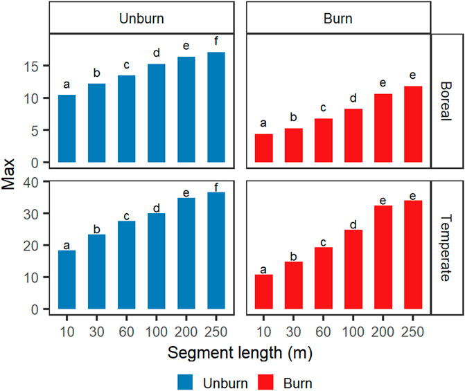
FIGURE 7. Comparisons of the maximum canopy height using non-parametric multiple comparisons test: the x-axis shows segment lengths and the y-axis shows averages maximum canopy height derived from the AGCH algorithm. Different letters mean the datasets are significantly different.

The canopy structures of the temperate forest and the boreal forest also have great differences. In Figure 5, the average value of maximum height at 100 m length is 30.09 m for the unburned temperate forest. However, for the boreal forest, the average maximum height at 100 m length is only 15.24 m for the unburned samples (Figure 6). Canopy coverage (cc) in the unburned temperate forest is 0.86 while it is 0.68 in the unburned boreal forest at 100 m length. Average values of canopy openness (openness) in the unburned temperate forest and boreal forest are 7.82 and 3.58 at 100 m length, respectively. These metrics indicate that the temperate forests are taller with higher canopy coverage and variations. However, structure changes in the boreal forest during fires were greater since the average values of most metrics decreased by more than 50% in Figure 8. Besides, the two algorithms present similar abilities to capture canopy structure changes as the relative changes (the ratio of differenced value and pre-fire value) are significantly correlated, r = 0.82 (p < 0.01) and 0.67 (p < 0.01) in the temperate forest and the boreal forest, respectively.

FIGURE 8

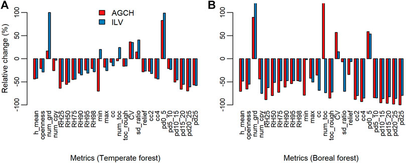
FIGURE 8. Relative changes [ = 100%*(average of burned samples–average of unburned samples)/average of unburned samples] of metrics in (A) the temperate forest and (B) the boreal forest using the AGCH algorithm and the ILV algorithm derived samples at 100 m segment length in strong beams.

Burned Forest Classification at Different Scales

The Random forest classification method was employed to classify the burned and the unburned segments in strong beams along ICESat-2 ground tracks. The overall accuracies are increasing at first when segment lengths get coarser in both the temperate forest and the boreal forest (Figure 9). When the segment length reaches 100 m, the classification accuracies start to saturate. For 200 and 250 m segment lengths, the accuracies are comparable or even lower than that of 100 m. Moreover, samples produced by both algorithms get good classification accuracies though the accuracies of the AGCH algorithm derived samples are slightly higher. For the boreal forest, the classification accuracies are higher than those of the temperate forest, which is due to greater canopy structure changes after fires (Figure 8). Table 2 illustrates that the accuracies of 100 m segment length and 30 m length are significantly different in the temperate forest, indicating the significant influence of spatial resolutions on burned forest classification. The accuracies of 100 m segments and 10 m segments are also significantly different in the temperate forest. For the boreal forest, the accuracies of 100 m segments are significantly different from those of 30 and 10 m segments.

FIGURE 9

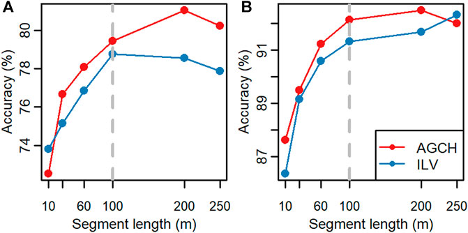
FIGURE 9. Accuracies of burned forest classification at different segment lengths based on the AGCH algorithm and the ILV algorithm derived samples using strong beams: (A) the temperate forest and (B) the boreal forest. The dash lines show the 100 m segment length.

TABLE 2

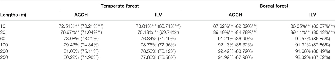
TABLE 2. Accuracies of burned forest classification along ICESat-2 ground tracks using segments derived from the AGCH and the ILV algorithms with strong beams, where the accuracies in parentheses come from weak beams. The Pair-wise proportion test in R, which can avoid family-wise error, was employed to compare the differences between classification accuracy of 100 m segments and accuracies of other segment lengths. * for p < 0.05, ** for p < 0.01 and *** for p < 0.001.

Classification results of burned segments along ICESat-2 ground tracks match the reference burn maps well (Figure 10), where segments are produced at 100 m segment length with strong beams. Segments derived from the two photon classification algorithms get similar classification results and comparable accuracies. The classification accuracies of burned vegetation in the boreal forest using samples from the AGCH algorithm and the ILV algorithm are 92.13 and 91.32%, respectively. For the temperate forest, the overall accuracies of burned segment classification using the AGCH and the ILV derived samples are 79.43 and 78.75%.

FIGURE 10

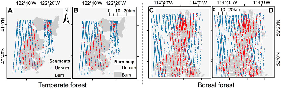
FIGURE 10. Classification results of the burned forest with strong beams at 100 m segment length using: samples in the temperate forest derived from (A) the AGCH and (B) the ILV algorithms; samples in the boreal forest derived from (C) the AGCH and (D) the ILV algorithms. Each segment was labeled by the location of its center most photon point.

Comparisons of Strong Beams and Weak Beams

Average values of the twenty-six canopy related metrics using weak beams are presented in Supplementary Figures S4–S7. These metrics vary along with spatial resolutions like those in strong beams, e.g. the maximum canopy height (max) increases along with coarser spatial resolutions. At 100 m segment length, we calculated the ratio of signal photons (ground photons and canopy photons) between strong beams and weak beams derived from the AGCH algorithm in the unburned temperate forest and the unburned boreal forest, 3.92 and 3.72, respectively, which are close to the designed energy ratio of 4:1. Less energy emitted from the ICESat-2/ATLAS instrument means fewer photons can get back, leading to fewer photon measurements in weak beams.

Figure 11 shows comparisons of typical canopy height related metrics such as RH50, RH75, RH95, cc2, and cc4 between samples from strong beams and weak beams at 100 m segment length. Metrics in weak beams are significantly higher than those in strong beams in the temperate forest based on samples from both the AGCH and the ILV algorithms. For the boreal forest, metrics in weak beams are significantly larger using the AGCH algorithm while smaller using the ILV derived samples. These metrics are significantly different comparing weak beams and strong beams, which indicates that point density impacts the measurements of canopy structures.

FIGURE 11

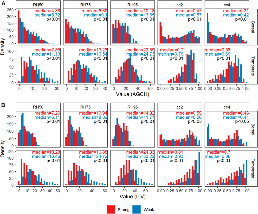
FIGURE 11. Comparisons of metrics from strong beams and weak beams based on samples derived from (A) the AGCH algorithm and (B) the ILV algorithm, where median means the median value of a metric and p is the significance between samples of weak beams and strong beams based on the Mann-Whitney test.

The classification accuracies of samples from both strong beams and weak beams are increasing along with spatial resolutions and saturate at 100 m segment length (Figure 12). Moreover, the accuracies of samples from the AGCH algorithm and the ILV algorithm have similar patterns. Based on Table 2, the differences of accuracies between 100 m segment length and other segment lengths are not significant except 30 and 10 m lengths, using weak beams in the temperate forest. For the boreal forest, the accuracy of 100 m segments is significantly different from those of 30 and 10 m segments. It is worth noting that, samples of weak beams always have lower accuracies than those of strong beams (Figure 12). This is due to lower point density since energy in weak beams is only ¼ of that in strong beams. With lower point density, it is more difficult to distinguish real ground points, canopy points, and noises, causing more errors in metrics calculation and burned forest classification.

FIGURE 12

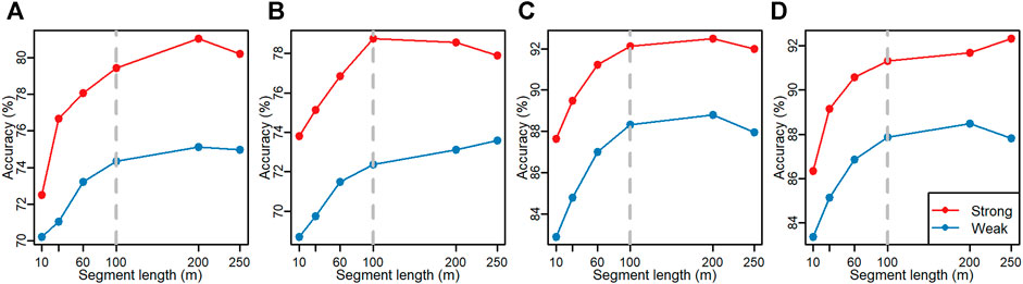
FIGURE 12. Accuracies of burned forest classification at different spatial resolutions using both weak beams and strong beams by: samples derived from (A) the AGCH and (B) the ILV algorithms in the temperate forest; samples derived from (C) the AGCH and (D) the ILV in the boreal forest. The dash lines show the 100 m segment length.

Discussion

Effects of Spatial Resolutions

This study focuses on the effects of spatial resolutions on burned forest classification using LiDAR data. ICESat-2 photon counting data were summarized at different segment lengths to match commonly adopted spatial resolutions, i.e., 10, 30, 60, 100, 200, and 250 m. The Random Forest method was employed for burned segment classification. As shown in Figures 5, 6, most canopy related metrics will change along with spatial resolutions, e.g., the number of canopy photons and maximum canopy height increase with coarser spatial resolutions. In fact, the maximum height starts from the mean canopy height (when each point is a segment) and converges to the highest point in the whole region (when the whole region is a segment) when spatial resolution gets coarsened. Overall, spatial resolution can influence canopy structures we detected. This reminds scientists that it is necessary to keep the same spatial resolutions when comparing structure changes or monitoring forest dynamics. Matching data with different spatial resolutions directly can produce misleading results.

Moreover, classification accuracies in both the temperate forest and the boreal forest are good (Figure 9), which demonstrates the capability of spaceborne LiDAR in capturing forest structure changes (Liu et al., 2020). The classification accuracies increase when spatial resolutions get coarser and then saturate at 100 m segment length. Although samples with 10 m spatial resolution can provide more detailed information, the corresponding classification accuracies are significantly lower. 100 m segment length provides good classification accuracy and relatively better spatial details than 200 and 250 m segment lengths. Furthermore, data derived from the two typical photon filtering algorithms, the AGCH and the ILV, present comparable accuracies and similar trends in burned forest classification. These results confirm that 100 m segment length is a good choice for burned forest classification using spaceborne LiDAR data. As for 30 m spatial resolution, scientists can selectively use it since the corresponding classification accuracies are still acceptable.

The impact of spatial resolution on burned forest classification is mainly due to its control on intra-class and inter-class canopy structure variabilities. When spatial resolution gets coarser, intra-class variability tends to decrease, contributing to higher classification accuracy (Roth et al., 2015). At fine spatial resolutions (e.g., 10 m), more detailed information can be recorded such as young trees with low canopy height or trees from different species, causing more variations in canopy structures (increase in intra-class variability) and lower classification accuracy. However, in coarse spatial resolutions (e.g., 100 m), a segment will cover multiple species or trees with different ages, wiping out variations caused by ages or species and decreasing intra-class variability. Thus, classification accuracies increase with coarser spatial resolutions. Jeffreys–Matusita (JM) distance is a commonly used metric in classification, which combines both intra-class variability and inter-class variability to analyze the separability of different classes (Wang and Glenn, 2009). The effective range of the JM distance is 0–1.4142, with large values for high separability. As shown in Figure 13, the JM distances increase along with coarser spatial resolutions, indicating an increase of inter-class variability and a decrease of intra-class variability, producing high separability.

FIGURE 13

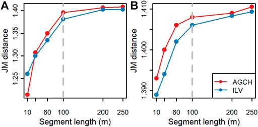
FIGURE 13. Jeffreys–Matusita (JM) distance of burned and unburned samples in strong beams at each segment length in (A) the temperate forest and (B) the boreal forest. The dash lines show the 100 m segment length.

Photon Point Density

The classification accuracies of burned forests with strong beams are higher than those of using weak beams in both the temperate forest and the boreal forest (Figure 12), which is mostly influenced by photon point density. Low photon point density leads to more errors in data processing, resulting in low classification accuracies. First, there are many noisy points caused by the solar background in ICESat-2/ATLAS photon counting data. It is difficult to effectively distinguish signal photons from background noises when point density is low since photon filtering algorithms, e.g., the AGCH and the ILV, leverage point density to kick out background noises. Second, the classification of photons into ground points and canopy points is challenging with low point density as ground photon points are always rare in forest regions, especially under a dense canopy. Low photon point density will directly decrease the number of ground points, increasing the possibility of misclassification. Thus, more canopy photons will be misclassified as ground points, causing errors in canopy structure detection. Third, photon point density itself is closely related to the accuracy of canopy characterization and biomass estimation (Singh et al., 2015). Singh et al. (2015) found that the accuracy of biomass estimation was good until the point density decreased under 40% of the original dataset. In Jakubowski et al. (2013), prediction accuracies of canopy related metrics were largely invariant at moderate to high pulse densities while declined at low densities. These results are consistent with the comparisons of classification accuracies using samples from strong beams and weak beams. Researchers should pay more attention to the effects of photon point density when using weak beams.

Limitations

In this study, different spatial resolutions are employed to summarize ICESat-2 photon counting LiDAR data and classify burned and unburned forest segments. Our results demonstrate that spatial resolutions can significantly impact the forest structures we detected and the accuracy of burned forest classification. However, due to the limitation of data availability (fire perimeters and high resolution reference burn maps), only the temperate forest and the boreal forest were adopted in the analysis. We thank that Canada and United States update their fire databases very quickly so that fire perimeters in the temperate forest and the boreal forest are available. We agree that other forest types, e.g., tropical forest or subtropical forest, are also very important in the biosphere. More forest types should be investigated in further studies, especially the tropical forest. We hope there will be more accurate and high resolution fire-related datasets available to support the science community.

Conclusion

This study is the first to analyze the effects of spatial resolution on burned forest classification using spaceborne LiDAR data. ICESat-2/ATLAS photon counting data were summarized at different segment lengths, i.e., 10, 30, 60, 100, 200, and 250 m, to match commonly used spatial resolutions. Two typical photon filtering algorithms, the AGCH and the ILV, were selected for data processing to avoid biases from a single algorithm. ICESat-2 data in the temperate forest in northern California, the United States, and the boreal forest in Alberta, Canada, were classified with the Random Forest method. Results show that canopy structure characterization is significantly influenced by spatial resolutions. The classification accuracies of burned forests increase along with coarser spatial resolutions and saturate at 100 m segment length. Moreover, the accuracies of burned forest classification based on strong beams are higher than those of weak beams. Segments derived from the two filtering algorithms get comparable classification accuracies. These findings demonstrate that spatial resolution will influence canopy characterization and fire monitoring. Furthermore, 100 m is a good choice for burned forest classification which provides decent classification accuracy and spatial details. As more spaceborne LiDAR data are available and accumulating, e.g., ICESat-2 data and GEDI data, further research studies can explore more applications of LiDAR data in fire management and extend the use of LiDAR data to applications in ecological recovery and carbon dynamics.

Data Availability Statement

The original contributions presented in the study are included in the article/Supplementary Material, further inquiries can be directed to the corresponding author.

Author Contributions

Conceptualization, ML and SP; Method, experiments, and writing original draft, ML; Funding source and manuscript revision, SP; Helping with data processing and manuscript revision, LM. All authors have read and agreed to the published version of the manuscript.

Funding

This research was funded by NASA’s ICESat-2 SDT (Grant # NNH19ZDA001N).

Conflict of Interest

The authors declare that the research was conducted in the absence of any commercial or financial relationships that could be construed as a potential conflict of interest.

Supplementary Material

The Supplementary Material for this article can be found online at: https://www.frontiersin.org/articles/10.3389/frsen.2021.666251/full#supplementary-material

References

Aragão, L. E. O. C., Anderson, L. O., Fonseca, M. G., Rosan, T. M., Vedovato, L. B., Wagner, F. H., et al. (2018). 21st Century Drought-Related Fires Counteract the Decline of Amazon Deforestation Carbon Emissions. Nat. Commun. 9, 536. doi:10.1038/s41467-017-02771-y

PubMed Abstract | CrossRef Full Text | Google Scholar

Balch, J. K., Bradley, B. A., Abatzoglou, J. T., Nagy, R. C., Fusco, E. J., and Mahood, A. L. (2017). Human-started Wildfires Expand the Fire Niche across the United States. Proc. Natl. Acad. Sci. USA 114, 2946–2951. doi:10.1073/pnas.1617394114

PubMed Abstract | CrossRef Full Text | Google Scholar

Breiman, L. (2001). Random Forests. Machine Learn. 45, 5–32. doi:10.1023/A:1010933404324

CrossRef Full Text | Google Scholar

Cattau, M. E., Wessman, C., Mahood, A., and Balch, J. K. (2020). Anthropogenic and Lightning‐started Fires Are Becoming Larger and More Frequent over a Longer Season Length in the U.S.A. Glob. Ecol Biogeogr 29, 668–681. doi:10.1111/geb.13058

CrossRef Full Text | Google Scholar

Chuvieco, E., Mouillot, F., van der Werf, G. R., San Miguel, J., Tanase, M., Koutsias, N., et al. (2019). Historical Background and Current Developments for Mapping Burned Area from Satellite Earth Observation. Remote Sensing Environ. 225, 45–64. doi:10.1016/j.rse.2019.02.013

CrossRef Full Text | Google Scholar

Cohen, W. B., Maiersperger, T. K., Yang, Z., Gower, S. T., Turner, D. P., Ritts, W. D., et al. (2003). Comparisons of Land Cover and LAI Estimates Derived from ETM+ and MODIS for Four Sites in North America: a Quality Assessment of 2000/2001 Provisional MODIS Products. Remote Sensing Environ. 88, 233–255. doi:10.1016/j.rse.2003.06.006

CrossRef Full Text | Google Scholar

Duncanson, L., Neuenschwander, A., Hancock, S., Thomas, N., Fatoyinbo, T., Simard, M., et al. (2020). Biomass Estimation from Simulated GEDI, ICESat-2 and NISAR across Environmental Gradients in Sonoma County, California. Remote Sensing Environ. 242, 111779. doi:10.1016/j.rse.2020.111779

CrossRef Full Text | Google Scholar

Fernandez-Manso, A., Quintano, C., and Roberts, D. A. (2019). Burn Severity Analysis in Mediterranean Forests Using Maximum Entropy Model Trained with EO-1 Hyperion and LiDAR Data. ISPRS J. Photogrammetry Remote Sensing 155, 102–118. doi:10.1016/j.isprsjprs.2019.07.003

CrossRef Full Text | Google Scholar

Fraser, R., Van der Sluijs, J., and Hall, R. (2017). Calibrating Satellite-Based Indices of Burn Severity from UAV-Derived Metrics of a Burned Boreal Forest in NWT, Canada. Remote Sensing 9, 279. doi:10.3390/rs9030279

CrossRef Full Text | Google Scholar

Fusco, E. J., Finn, J. T., Abatzoglou, J. T., Balch, J. K., Dadashi, S., and Bradley, B. A. (2019). Detection Rates and Biases of Fire Observations from MODIS and agency Reports in the Conterminous United States. Remote Sensing Environ. 220, 30–40. doi:10.1016/j.rse.2018.10.028

CrossRef Full Text | Google Scholar

García, M., Popescu, S., Riaño, D., Zhao, K., Neuenschwander, A., Agca, M., et al. (2012). Characterization of Canopy Fuels Using ICESat/GLAS Data. Remote Sensing Environ. 123, 81–89. doi:10.1016/j.rse.2012.03.018

CrossRef Full Text | Google Scholar

Garcia, M., Saatchi, S., Casas, A., Koltunov, A., Ustin, S., Ramirez, C., et al. (2017). Quantifying Biomass Consumption and Carbon Release from the California Rim Fire by Integrating Airborne LiDAR and Landsat OLI Data. J. Geophys. Res. Biogeosci. 122, 340–353. doi:10.1002/2015JG003315

PubMed Abstract | CrossRef Full Text | Google Scholar

Gibson, R., Danaher, T., Hehir, W., and Collins, L. (2020). A Remote Sensing Approach to Mapping Fire Severity in South-Eastern Australia Using sentinel 2 and Random forest. Remote Sensing Environ. 240, 111702. doi:10.1016/j.rse.2020.111702

CrossRef Full Text | Google Scholar

Goetz, S. J., Sun, M., Baccini, A., and Beck, P. S. A. (2010). Synergistic Use of Spaceborne Lidar and Optical Imagery for Assessing forest Disturbance: An Alaska Case Study. J. Geophys. Res. 115, a–n. doi:10.1029/2008JG000898

CrossRef Full Text | Google Scholar

Gwenzi, D., Lefsky, M. A., Suchdeo, V. P., and Harding, D. J. (2016). Prospects of the ICESat-2 Laser Altimetry mission for savanna Ecosystem Structural Studies Based on Airborne Simulation Data. ISPRS J. Photogrammetry Remote Sensing 118, 68–82. doi:10.1016/j.isprsjprs.2016.04.009

CrossRef Full Text | Google Scholar

Hawbaker, T. J., Vanderhoof, M. K., Schmidt, G. L., Beal, Y.-J., Picotte, J. J., Takacs, J. D., et al. (2020). The Landsat Burned Area Algorithm and Products for the Conterminous United States. Remote Sensing Environ. 244, 111801. doi:10.1016/j.rse.2020.111801

CrossRef Full Text | Google Scholar

Jakubowski, M. K., Guo, Q., and Kelly, M. (2013). Tradeoffs between Lidar Pulse Density and forest Measurement Accuracy. Remote Sensing Environ. 130, 245–253. doi:10.1016/j.rse.2012.11.024

CrossRef Full Text | Google Scholar

Leigh, H. W., Magruder, L. A., Carabajal, C. C., Saba, J. L., and McGarry, J. F. (2015). Development of Onboard Digital Elevation and Relief Databases for ICESat-2. IEEE Trans. Geosci. Remote Sensing 53, 2011–2020. doi:10.1109/TGRS.2014.2352277

CrossRef Full Text | Google Scholar

Liu, M., Popescu, S., and Malambo, L. (2020). Feasibility of Burned Area Mapping Based on ICESAT−2 Photon Counting Data. Remote Sensing 12, 24. doi:10.3390/rs12010024

CrossRef Full Text | Google Scholar

Liu, M., and Yang, L. (2020). Human-caused Fires Release More Carbon Than Lightning-Caused Fires in the Conterminous United States. Environ. Res. Lett. 16, 014013. doi:10.1088/1748-9326/abcbbc

CrossRef Full Text | Google Scholar

Maxwell, A. E., Warner, T. A., and Fang, F. (2018). Implementation of Machine-Learning Classification in Remote Sensing: an Applied Review. Int. J. Remote Sensing 39, 2784–2817. doi:10.1080/01431161.2018.1433343

CrossRef Full Text | Google Scholar

Montealegre, A., Lamelas, M., Tanase, M., and de la Riva, J. (2014). Forest Fire Severity Assessment Using ALS Data in a Mediterranean Environment. Remote Sensing 6, 4240–4265. doi:10.3390/rs6054240

CrossRef Full Text | Google Scholar

Neuenschwander, A., and Pitts, K. (2019). The ATL08 Land and Vegetation Product for the ICESat-2 Mission. Remote Sensing Environ. 221, 247–259. doi:10.1016/j.rse.2018.11.005

CrossRef Full Text | Google Scholar

Popescu, S. C., Zhou, T., Nelson, R., Neuenschwander, A., Sheridan, R., Narine, L., et al. (2018). Photon Counting LiDAR: An Adaptive Ground and Canopy Height Retrieval Algorithm for ICESat-2 Data. Remote Sensing Environ. 208, 154–170. doi:10.1016/j.rse.2018.02.019

CrossRef Full Text | Google Scholar

Reese, H., Nilsson, M., Sandström, P., and Olsson, H. (2002). Applications Using Estimates of forest Parameters Derived from Satellite and forest Inventory Data. Comput. Electron. Agric. 37, 37–55. doi:10.1016/S0168-1699(02)00118-7

CrossRef Full Text | Google Scholar

Rödig, E., Knapp, N., Fischer, R., Bohn, F. J., Dubayah, R., Tang, H., et al. (2019). From Small-Scale forest Structure to Amazon-wide Carbon Estimates. Nat. Commun. 10, 1–7. doi:10.1038/s41467-019-13063-y

PubMed Abstract | CrossRef Full Text | Google Scholar

Roteta, E., Bastarrika, A., Padilla, M., Storm, T., and Chuvieco, E. (2019). Development of a Sentinel-2 Burned Area Algorithm: Generation of a Small Fire Database for Sub-saharan Africa. Remote Sensing Environ. 222, 1–17. doi:10.1016/j.rse.2018.12.011

CrossRef Full Text | Google Scholar

Roth, K. L., Roberts, D. A., Dennison, P. E., Peterson, S. H., and Alonzo, M. (2015). The Impact of Spatial Resolution on the Classification of Plant Species and Functional Types within Imaging Spectrometer Data. Remote Sensing Environ. 171, 45–57. doi:10.1016/j.rse.2015.10.004

CrossRef Full Text | Google Scholar

Schoennagel, T., Balch, J. K., Brenkert-Smith, H., Dennison, P. E., Harvey, B. J., Krawchuk, M. A., et al. (2017). Adapt to More Wildfire in Western North American Forests as Climate Changes. Proc. Natl. Acad. Sci. USA 114, 4582–4590. doi:10.1073/pnas.1617464114

PubMed Abstract | CrossRef Full Text | Google Scholar

Singh, K. K., Chen, G., McCarter, J. B., and Meentemeyer, R. K. (2015). Effects of LiDAR point Density and Landscape Context on Estimates of Urban forest Biomass. ISPRS J. Photogrammetry Remote Sensing 101, 310–322. doi:10.1016/j.isprsjprs.2014.12.021

CrossRef Full Text | Google Scholar

Wang, C., and Glenn, N. F. (2009). Estimation of Fire Severity Using Pre- and post-fire LiDAR Data in Sagebrush Steppe Rangelands. Int. J. Wildland Fire 18, 848. doi:10.1071/WF08173

CrossRef Full Text | Google Scholar

Zwally, H. J., Schutz, B., Abdalati, W., Abshire, J., Bentley, C., Brenner, A., et al. (2002). ICESat's Laser Measurements of Polar Ice, Atmosphere, Ocean, and Land. J. Geodynamics 34, 405–445. doi:10.1016/S0264-3707(02)00042-X

CrossRef Full Text | Google Scholar