Planetary Boundary Layer Height Estimates From ICESat-2 and CATS Backscatter Measurements

Introduction

The Planetary Boundary Layer (PBL) is the lowest region of the atmosphere in contact with the surface that controls the complex interactions between the surface (land and ocean) and the free troposphere. Ranging in depth from just a few hundred meters to near 6 km, moisture, heat and pollutants at the surface are transferred into the atmosphere within the PBL and are transported to other regions of the atmosphere mainly by turbulence and convective motions. Since the PBL contains a large percentage of the total atmospheric moisture, it determines to a large degree the amount of latent heat available to fuel deep convection and storm development. Our understanding of air quality, human health, and severe storms are currently hindered by an incomplete understanding of PBL processes. The height of the PBL (PBLH) is an essential aspect of Earth’s coupled system that must be represented properly in weather, climate, and air quality prediction models. PBLH varies as a function of regional land and ocean characteristics, seasonal atmospheric patterns, and diurnal solar heating. This variability is a critical indicator of regional surface-atmosphere energy, mass, and momentum exchanges that strongly influence convection, precipitation, air pollution, and extreme events.

Because of its importance, much attention has been given to PBL research over the last many decades. The interaction of the boundary layer with the overlying troposphere is extremely important to the accuracy of numerical weather prediction models. This is particularly apparent in regions of coastal or oceanic cyclogenesis. Over 40 years ago, Bosart (1981) and Tracton (1973) found that the existing weather prediction models of the time did not satisfactorily incorporate the interaction of the PBL with the troposphere as a major source of energy for developing cyclones. In a study of the 1979 President’s Day east coast blizzard, Bosart (1981) concluded that the failure to correctly model the effect of convective scale processes and oceanic heat and moisture flux in the boundary layer is a major cause of operational prediction model’s inability to simulate oceanic and coastal cyclogenesis and storm intensity.

PBLH is defined in a number of different ways and can differ depending on the technique used to measure it. The standard or thermodynamic approach utilizes radiosonde measurements of temperature and moisture. In a convective boundary layer, heated from below, PBLH is usually defined as that height where the potential temperature profile increases abruptly with height while at the same altitude, the relative humidity decreases significantly. Note however, that any single measurement of the depth of a convective boundary layer will depend on where the measurement was made with respect to the convective cells (updrafts and downdrafts). The convective PBL top over a given horizontal distance varies and is higher at the position of updrafts and lower in regions of downdrafts. The region between the lowest and highest PBLH in a local convective boundary layer is called the entrainment zone. (Melfi et al., 1985). For a stable boundary layer, characterized by a temperature inversion at the surface, PBLH is defined as the height of the top of the inversion (Stull 1988). The convective PBLH can be estimated using lidar and sodar since the PBL generally contains more aerosol than the free troposphere above. Lidar can detect this gradient of aerosol concentration (since backscatter magnitude is related to aerosol number density) or PBL cloud top heights, and the height at which these occur is defined as the PBLH. The detection of PBLH in stable boundary layers using satellite lidar is more difficult for a number of reasons including a small or non-existent aerosol gradient at the layer top, masking of the layer by the previous daytime PBL and the often very shallow nature of nocturnal or stable layers. Common methods used to detect PBLH using lidar include the backscatter threshold method (Melfi et al., 1985; Palm et al., 2005), maximum variance (Jordan et al., 2010; McGrath-Spangler and Denning, 2012), Haar wavelet (Davis et al., 1997; Cohn and Angevine 2000) and backscatter gradient method (Van Pul et al., 1994).

PBLH estimates from space-based lidar systems have provided critical data for 1) determining regional and seasonal PBLH variability, 2) comparisons with other definitions of PBLH, and 3) evaluation of PBLH in regional and global models. Jordan et al. (2010) compared PBLH derived from CALIPSO (The Cloud-Aerosol Lidar and Infrared Pathfinder Satellite Observation) backscatter profiles with co-located (temporally and spatially) PBLH from the NASA Goddard GEOS-5 MERRA (The Modern Era Reanalysis for Research and Applications (MERRA) (Rienecker et al., 2008) reanalysis product. The model PBLH was defined by the lowest model level for which the turbulent diffusion coefficient drops below 2 m²s⁻¹ when values above this threshold exist in the lowest two levels of the column. They note this threshold is somewhat arbitrary but it represents turbulent intensity roughly two orders of magnitude below typical peak values (∼100 m²/s) in a strongly convective model PBL. Jordan et al. (2010) found that the model PBLH was higher than CALIPSO retrievals over much of the equatorial pacific but over north Africa, the converse was true. Over daytime Sahara, for instance, where CALIPSO measured PBLH near 6 km, the model values were roughly half of that. McGrath-Spangler and Denning (2012) compared PBL depths estimated from CALIPSO (Cloud-Aerosol Lidar and Infrared Pathfinder Satellite Observation) lidar backscatter measurements with model reanalysis and AMDAR (Aircraft Meteorological DAta Reporting) estimates. They found that lidar-based estimates of PBL depth tend to be shallower than aircraft estimates in coastal areas and compared to model reanalysis were greater over the oceans and areas of the boreal forest and shallower over the arid and semiarid regions of North America. Liu et al. (2015) compared ECMWF PBLH with that derived from CALIPSO over the China region and found that the CALIPSO heights were generally higher than ECMWF. The CALIPSO PBL heights were obtained through analysis of the 532 nm backscatter profiles using the maximum variance method after cloud clearing using the level 2 vertical feature mask. The ECMWF model defines the top of the PBL as the level where the bulk-Richardson number, based on the difference between quantities at that level and the lowest model level, reaches a critical value of 0.25.

Estimates of PBLH from backscatter lidars have been identified as an important part of the program of record both currently and as part of a future PBL global observing system (Teixeira et al., 2021). In this paper we use data from the Cloud-Aerosol Transport System (CATS) and the Ice Cloud and land Elevation Satellite-2 (ICESat-2) to estimate PBLH using two methods: 1) a modified backscatter threshold method and 2) a machine learning technique using Convolutional Neural Network (CNN) methods. The results will be compared with each other and with data from radiosondes and MERRA-2 reanalysis PBL height. Data and Methods will describe the data used for the analysis and a description of the PBLH retrieval algorithms. PBLH retrieval results and comparisons with observations is given in Results with conclusions and summary in Summary and Conclusion.

Data and Methods

CATS

The Cloud-Aerosol Transport System (CATS) operated on the International Space Station (ISS), primarily at the 1,064 nm wavelength, for 33 month (05 February 2015 to 29 October 2017). The CATS instrument was designed to both demonstrate new technologies for future space-based lidar missions and provide valuable Earth science remote sensing data from the ISS through vertical profiles of clouds and aerosols (McGill et al., 2015). This paper uses the CATS Level 1B data products, V3-00, which were released in October 2018. The primary parameters of interest in the CATS Level 1B data product are the 1) attenuated total backscatter (ATB) coefficient, 2) attenuated perpendicular backscatter (APB) coefficient (both with units of km⁻¹ sr⁻¹), and 3) linear volume depolarization ratio (Yorks et al., 2016). These parameters are provided at the 1,064 nm wavelength at a horizontal resolution of 350 m (along-track) and vertical resolution of 60 m. CATS data products have been utilized to study aerosol impacts on the climate system (Rajapakshe et al., 2017; Christian et al., 2019) and aerosol transport (Hughes et al., 2016; McGill et al., 2020; O’Sullivan et al., 2020).

CATS data is well suited for PBLH detection and has the potential for determining the diurnal variability of the PBLH on seasonal and regional scales (because its orbit is not sun-synch). CATS provides robust 1,064 nm attenuated backscatter data with high 1,064 nm signal-to-noise ratio (SNR), especially at nighttime (Pauly et al., 2019). This SNR results in low minimum detectable backscatter (MDB), the lowest backscatter value that PBL clouds and the aerosol mixing height can be detected (Yorks et al., 2016). Additionally, the total backscatter signal at 1,064 nm has a smaller molecular contribution, especially near the surface, compared to longer wavelengths (Yorks et al., 2021). CATS also observed different local times each overpass, covering the full diurnal cycle roughly every 60 days due to the 51.8° inclination angle of the ISS orbit. This sampling enabled several investigations of cloud and aerosol seasonal, regional, and diurnal variability (Noel et al., 2018; Chepfer et al., 2019; Lee et al., 2019; Yu et al., 2021).

The Ice, Cloud and land Elevation Satellite-2

The Ice, Cloud and land Elevation Satellite (ICESat), which operated from 2003 until 2009 was the first satellite lidar to study the earth’s surface and atmosphere (Abshire et al., 2005; Spinhirne et al., 2005). ICESat-2, the successor to ICESat, was launched into a 92° inclination, precessing orbit in September of 2018 and has been in continuous operation since October of that year (Abdalati et al., 2010; Markus et al., 2017). Like CATS, ICESat-2 is not in a sun-synchronous orbit and thus can examine diurnal changes of the quantities it measures. ICESat-2 carries only one instrument–the Advanced Topographic Laser Altimeter System (ATLAS) that utilizes a high repetition rate (10 KHz), low per pulse energy (500 µJ), 532 nm laser and photon counting detectors. Though specifically designed and optimized to obtain high resolution altimetry measurements of the Earth’s surface, ICESat-2 also has an atmospheric channel to record backscatter from clouds and aerosols from 14 km altitude to the surface at a horizontal and vertical resolution of 280 and 30 m, respectively.

ATLAS employs a diffractive optical element (DOE) to split the laser pulse into 6 individual beams that are simultaneously emitted from the satellite. Three of the beams have nominal energies of about 25 μJ per pulse (weak beams) and the other 3 have energies roughly 4 times the weak beams (strong beams). The altimetry measurements utilize all 6 laser beams while for the atmospheric measurements, backscatter data are captured only from the 3 strong beams. Each strong/weak beam pair is separated by about 3 km on the ground (across track). The ICEsat-2 data used in this paper for the retrieval of PBLH are the average of the calibrated backscatter from the 3 strong beams stored on the version 004 ATL09 data product. For more information on the ICESat-2 atmospheric data products, please see Palm et al. (2020) and Palm et al. (2021).

Description of Algorithms

As mentioned in the introduction, there have been numerous approaches used to retrieve PBLH from ground based and satellite lidar. Here we employ and compare the results of two techniques. The first is a modified version of a technique first used in Melfi et al. (1985) called the threshold technique. This method is based on establishing a backscatter threshold and then searching the lidar profile from just above the surface upward for the height where the backscatter magnitude falls below the threshold value. The second is a machine learning technique that uses the output of the first method to “train” a neural network to identify where the PBL top is most likely located.

Threshold Method

The threshold method was first applied to aircraft lidar data obtained during the MASEX field campaign (Melfi et al., 1985) and subsequently used for PBLH estimation using data from GLAS (Geoscience Laser Altimeter System) aboard ICESat (Palm et al., 2005). A modified version of that algorithm is used here. The algorithm consists of two steps: 1) a long-distance horizontal averaging of the backscatter profiles to find a low resolution (called coarse) PBLH and 2) a shorter-distance horizontal averaging of the profiles comprising the coarse average, that are then searched in a narrow vertical window centered on the coarse average PBLH for a higher resolution (called fine) PBLH. The coarse and fine horizontal averaging distances depend on the solar elevation angle. Since both CATS and ICESat-2 have markedly lower signal to noise ratios in daylight than in nighttime, the daytime (solar elevation angle >0) averaging distance is much larger than that of nighttime (solar elevation angle <0). For the coarse averaging distance, we used 64 and 24 km, for daytime and nighttime, respectively. The fine averaging distance is 1/8 of the coarse averaging distance. This process results in a PBLH horizontal resolution of 8 and 3 km for daytime and nighttime, respectively. During the data averaging process, the backscatter profiles are vertically re-aligned such that the ground bin is always in the same bin. This is very important when averaging data in rough or mountainous terrain because if this is not done, surface signal can contaminate the lower few hundred meters of the profile and cause erroneous retrievals. In addition, for ICESat-2, folding of atmospheric scattering above 15 km to the 0–3 km altitude can be a problem in the tropics (see Palm et al., 2021 for more information). The cloud folding flag present on the ATL09 data product is used to filter out profiles suspected of containing significant folding in the coarse averaging process.

After the coarse averaging, the profile backscatter average between 200 and 400 m above the surface (S₃₀₀) is compared with a predefined threshold (T₃₀₀). For T₃₀₀ we used a value of 1.0 × 10⁻⁶ m⁻¹sr⁻¹ for ICESat-2 and 1.0 × 10⁻⁷ m⁻¹sr⁻¹ for CATS (since CATS uses 1,064 nm and the molecular scattering is an order of magnitude less at that wavelength). If S₃₀₀ is less than T₃₀₀, then no attempt is made to detect the PBLH for that average profile (PBLH is set to zero). This condition occurs when there are enough overlying opaque clouds present through the coarse average distance to have significantly attenuated the signal. If the 200–400 m average is greater than T₃₀₀, the profile is examined starting at 300 m above the surface and proceeding upward until two consecutive bins fall below a second threshold (T_top) defined as 0.70xS₃₀₀. If this condition occurs below 7 (4) km above the surface over land (water), the first (lower in height) bin of the 2 consecutive bins determines the PBLH. If this condition is not reached within 7 (or 4) km of the surface, then PBLH is set to zero. If the resulting PBLH at the coarse resolution is non-zero, it is then used to define a vertical window 1 km wide around which the fine average profiles are searched for the PBLH. The fine search begins at the bottom of the 1 km wide window and proceeds upward, again searching for 2 consecutive bins that fall below T_top. If found below the window top, the fine PBLH is set to the first (lower) of the 2 bins. If it is not found before reaching the top of the window, the fine PBLH is set to the coarse average PBLH. If the coarse PBLH is zero, all corresponding fine PBLH are set to zero.

Convolutional Neural Network Method

A convolutional neural network (CNN) was trained to estimate PBLH using the PBLH determined from CATS data using the more traditional threshold technique and the raw (photon counts) CATS 1064 nm data as input. For this study, 1 month of CATS data was used as the “truth” dataset, enough for the CNN to accurately estimate PBLH from the CATS data. One month of data was chosen because it was large enough to contain a representative sampling of PBL cloud and aerosol scenes that are representative of the PBLH, yet small enough to train the CNN relatively quickly. Previously published studies that trained CNN models suggest using a training dataset that is ∼20% of your prediction dataset provides accurate predictions (Shahin et al., 2004; Yorks et al., 2021). Supervised machine learning algorithms, such as CNN, have been utilized for feature recognition and object detection in images for years (Gidaris and Komodakis, 2015). While CNN techniques have been used for other Earth Science applications (Maskey et al., 2018; Pradhan et al., 2018), these are the first published results of CNN PBLH predictions using space-based lidar data. One advantage of the CNN technique is that the predictions are fast compared to more traditional techniques [20 s to process a single CATS data file (one half orbit)], although the training of the CNN model can take more time (3–5 h).

The CNN architecture and training method used in this study to estimate PBLH were similar to what was defined in Yorks et al. (2021). However, there were some key differences. The primary difference was how the training dataset was created. The entire PBL (not exclusively the top) was labeled in the raw CATS image by interpolating between points determined by the threshold approach described in The Threshold Method Section. Up-sampled CATS Level 2 data were used to assist in giving more realistic definition to the PBL shape in the raw lidar image. Areas where the lidar signal was attenuated, or the threshold approach did not determine a PBL height were filtered out. The other difference between the methodology in Yorks et al. (2021) is that here binary feature classification was used as opposed to multiple feature classification; however, this only implies an adjustment to the output layer of the CNN. The training dataset of PBLH defined by the threshold technique had horizontal resolutions of 7 km (night) and 80 km (day), different than the resolutions described in Threshold Method.

The CNN technique is able to match the accuracy of the threshold technique, at night, but at much finer horizontal resolutions. Figure 1A shows the 1,064 nm CATS attenuated total backscatter (km⁻¹ sr ⁻¹) for a nighttime scene over the middle of the Pacific Ocean where marine aerosols and PBL clouds are present, with the PBLH from the threshold technique (red dots) and CNN (yellow dots) overlaid. Both techniques appear to be accurately predicting the PBLH, as the red and yellow dots align well with the tops of the PBL clouds and marine aerosol layer present in the backscatter image. The difference in PBLH between the two techniques (CNN-threshold) is plotted in Figure 1B. On average, the two techniques agree to 228.8 m (absolute mean difference). The root mean square difference (RMSD) for this case is 301.2 m. This agreement is impressive given the CNN predictions are made at a horizontal resolution of 350 m, a factor of 10–20 improvement compared to the horizontal resolution of 3–8 km used in the traditional threshold technique. The CNN model uses the spatial correlation of the raw CATS signal at raw horizontal resolution (350 m), searching for the types of gradients that the threshold technique has related to the PBLH. Differences between the two techniques are expected since the finer resolution of the CNN model prevents the surface and cloud smoothing issues in the threshold technique, and, in some cases, the spatial correlation can overcome scenes with lower SNR. Yorks et al. (2021) showed that the CNN model increased the number of layers detected in CATS data (any resolution) by 30%, and enabled detection of 40% more atmospheric features at finer horizontal resolutions.

FIGURE 1

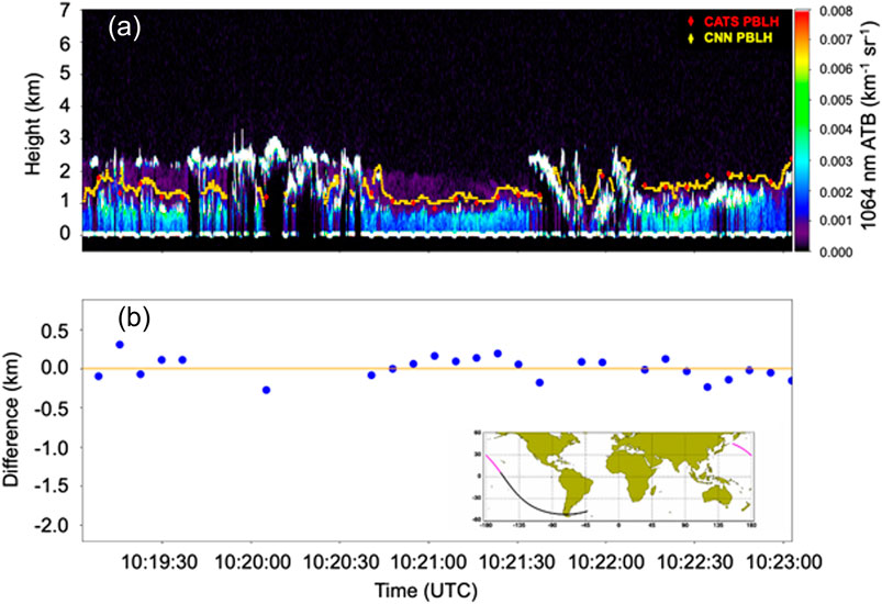
FIGURE 1. (A) CATS 1064 nm attenuated total backscatter along the track shown in the map inset for June 17, 2015 at roughly 10:21 UTC with the PBL height overlaid from the threshold (red dots) and CNN (yellow dots) techniques. (B) The difference (CNN-threshold) for the two techniques for the same scene.

The fine resolution of the CNN predications enables more accurate detection of the PBLH during complex scenes in daytime CATS data. The 1,064 nm CATS attenuated total backscatter (km⁻¹ sr⁻¹) for a daytime scene over the Atlantic Ocean and just off the west coast of Africa is shown in Figure 2A. As CATS approaches Africa it observes marine PBL clouds (12:14-12:15 UTC), then a marine aerosol layer with a lofted dust layer above at an altitude of 2–4 km from 12:15 to 12:17 UTC. The PBLH from both techniques match well with the tops of the PBL clouds and properly ignore the dust aerosols lofted into the free troposphere. There is very good agreement between the two techniques for this part of the scene, as shown in Figure 2B, even with the factor of 20 finer horizontal resolution employed by the CNN method. The mean absolute error is 96.0 m and the RMSE is 117.0 m. However, the mean error is 1.7 km and RMSE is 2.2 km from 12:17:30 to 12:19:00 UTC, where a complex cloud scene is observed by CATS. The threshold technique estimates a PBLH that is higher than the CNN method and the clouds visible in the CATS 1064 nm ATB image. This is likely the result of the coarse horizontal averaging required by the threshold technique (80 km) for this daytime scene, which artificially smeared these clouds, resulting in higher PBLH detections. The finer resolution of the CNN technique predictions enabled PBLH estimates that appear more accurate, given they better align with the cloud tops visible in the CATS 1064 nm ATB image. However, this CNN technique is not without limitations. During daytime over land, the lower SNR of the CATS 1064 nm data reduces the accuracy of the technique and often prevents an estimate from being predicted.

FIGURE 2

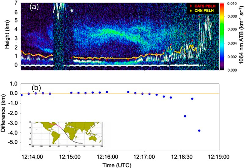
FIGURE 2. (A) CATS 1064 nm attenuated total backscatter along the track shown in the map inset for September 15, 2015 at 12:14-12:19 UTC with the PBL height overlaid from the threshold (red dots) and CNN (yellow dots) techniques. (B) The difference (CNN-threshold) for the two techniques for the same scene.

Results

Threshold Algorithm

We have run the threshold algorithm on four case studies where the ICESat-2 satellite orbit track comes within 20 km of a radiosonde station and within roughly an hour or two of the sonde launch. Though here we show the results of only two of the cases, the other two results are very similar. Figure 3A displays the calibrated backscatter for a nighttime ICESat-2 pass that comes within 20 km of the radiosonde station at La Paz, Mexico (latitude 24.11, longitude −110.32) on October 16, 2018. Drawn on the backscatter image are the coarse (red) and fine (yellow) PBL heights from the threshold algorithm. The potential temperature and relative humidity sounding, acquired at 12 UTC, is shown in Figure 3B. The time of the ICEsat-2 overpass at this location was about 10:59 UTC (4:59 AM local time). The PBL top as indicated by the temperature and moisture profiles is shown as the horizontal red dashed line. The approximate location of the point along the ICESat-2 track that is closest to the radiosonde station is indicated by the vertical white line on the backscatter image in Figure 3A. Generally, the well mixed, convective PBL top is indicated by an abrupt increase of potential temperature with height and a corresponding drop in the relative humidity. In Figure 3B this occurs at about 1.8 km. The three PBL top retrievals from the threshold algorithm closest to the radiosonde give heights of 1.8. 2.0 and 2.1 km. The higher two heights are likely influenced by the cumulus cloud between 310 and 330 km on the x axis. Such PBL height variability is not uncommon over a distance of 40–50 km.

FIGURE 3

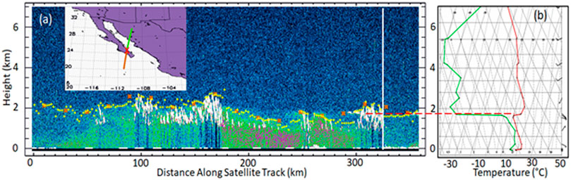
FIGURE 3. (A) ICESat-2 calibrated backscatter along the track shown in the map inset for October 16, 2018 at roughly 10:59 UTC with coarse (red asterisks) and fine (yellow plus signs) PBL height overlain. (B) The potential temperature (red) and relative humidity (green) from the La Paz, Mexico radiosonde at 12:00 UTC. The position of La Paz is marked on the map with a red ‘x” and the white vertical line in (A) marks the closest approach of ICESat-2 to La Paz.

Figure 4 is the same as Figure 3 but displays data for a daytime ICESat-2 pass that came within 20 km of the radiosonde station at Chichijima, Japan (latitude 27.09, longitude 142.19) on January 10, 2019. The sounding, shown in Figure 4B, was acquired at 00 UTC and the ICEsat-2 overpass was at 01:45 UTC (10:45 AM local time). The top of the PBL as indicated by the potential temperature and relative humidity is near 1.9 km (red, dashed horizontal line). The PBL height as retrieved form the ICESat-2 backscatter using the threshold algorithm at the point nearest the sonde location is about 2.0 km. The results shown in Figures 3, 4, and others not shown here, indicate that the threshold algorithm performs well for both nighttime and daytime PBL height retrieval using ICESat-2 data.

FIGURE 4

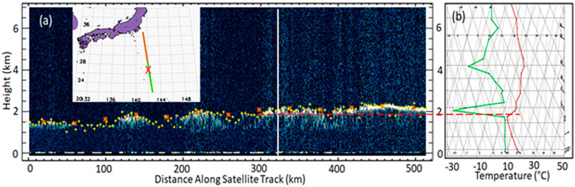
FIGURE 4. (A) Same as Figure 3 except for an ICESat-2 pass on January 10, 2019 at 01:45 UTC over Chichijima, Japan and (B) the Chichijima radiosonde temperature (red) and moisture profile (green) at 00 UTC.

The threshold algorithm was also applied to CATS L1B 1064 nm calibrated backscatter data. Because the CATS wavelength is 1,064 nm (ICESat-2 is 532 nm), the threshold limit (T₃₀₀ defined in Threshold Method) is smaller by a factor of 10. Other than that adjustment, no changes were made to the algorithm before it was run on the CATS data. Note also that the CATS vertical resolution is 60 m versus 30 m for ICEsat-2. Figure 5A shows an image of CATS data over the Caribbean on June 1, 2017 at 07:22 UTC (04:10 local time) and Figure 5B is a transect over the central Pacific that passes just east of Hawaii on June 1, 2017 at 11:55 UTC (01:55 Hawaii local time). The yellow + signs represent the coarse PBLH retrievals from the threshold algorithm.

FIGURE 5

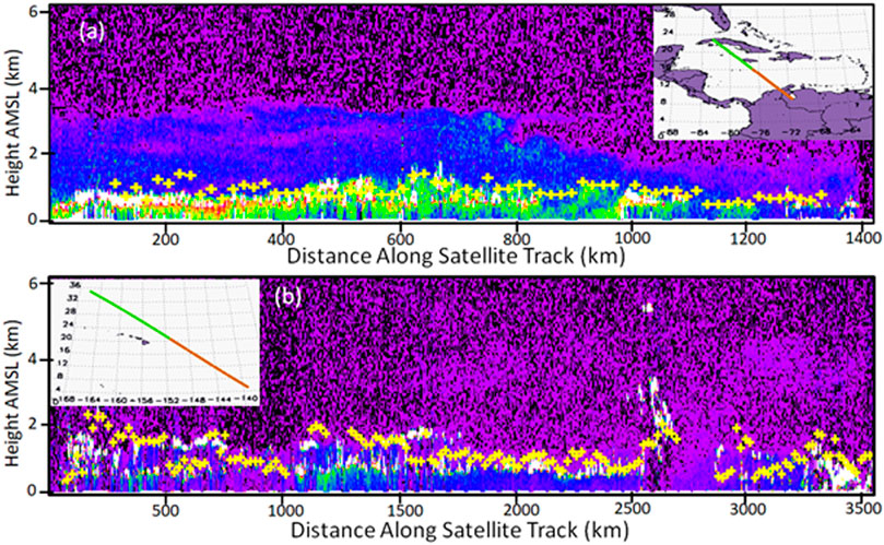
FIGURE 5. (A) CATS calibrated 1,064 nm backscatter data over the south Caribbean Sea on June 1, 2017 showing a marine PBL embedded in a thicker aerosol layer. (B) CATS calibrated 1,064 nm backscatter for a transect over the Pacific Ocean passing just east of Hawaii on June 1, 2017. The coarse PBL top as retrieved from the threshold algorithm is indicated by the yellow plus signs on both images.

Results shown in Figure 5A demonstrate the ability to resolve the relatively small aerosol gradient at the top of the marine PBL which is embedded in an elevated aerosol layer (possibly of Saharan origin). This is sometimes difficult for algorithms to do but is imperative for an accurate retrieval of PBLH. Figure 5B shows a typical open-ocean marine PBL that likely consists of two distinct layers–the shallower well mixed layer about 800–1,000 m thick capped by a weak inversion and a higher layer capped by the trade wind inversion at around 2 km. Evidence of this double inversion structure is seen in the 12 UTC June 1, 2017 radiosonde from Lihue, Hawaii (not shown) and is a typical occurrence over much of the open ocean.

The threshold algorithm has been run on the entire year of 2019 ICESat-2 data, comprised of 5,084 orbits, to create a global map of PBLH. The result is displayed in Figure 6, grouped by season and displayed on a 2 × 2 degree grid. The PBL heights range from about 800 m to 1.5 km over ocean and do not change much from season to season, but it is noted that in the winter hemisphere the PBL heights are higher over ocean, especially in the northern hemisphere east of continents. This is mainly due to the larger air-sea temperature difference causing higher surface heat flux and convection. The low PBL heights over ocean just west of continents is expected and plainly seen in the data. This is generally due to the upwelling of cold water which suppresses convection. These features are consistent with those noted by McGrath-Spangler and Denning (2013). Over land PBLH ranges from 2 to 3 km, with higher values over desert and arid regions during summer. Note that both night and day are used here for PBLH retrieval and that during nighttime over land, the lidar will largely be discerning the residual (daytime) PBL layer from the day before. At night the threshold technique using the CATS and ICESat-2 data is unable to retrieve the nocturnal layer due to its shallow depth and weak aerosol gradient at its top. Nighttime satellite PBL retrievals over land largely detect the top of the prior days convective PBL. Because of this fact, when comparing the ICESat-2 and CATS PBLH over land with model PBLH estimates, it is best to compare with the model data valid at mid-afternoon local time (∼2PM). While there are techniques to differentiate the nocturnal stable and residual layers, they have only been applied to ground-based lidar systems that are located near (10 s of meters) these layers, giving them higher signal-to-noise ratio and enabling layer detection at finer spatial resolutions (Lewis et al., 2013).

FIGURE 6

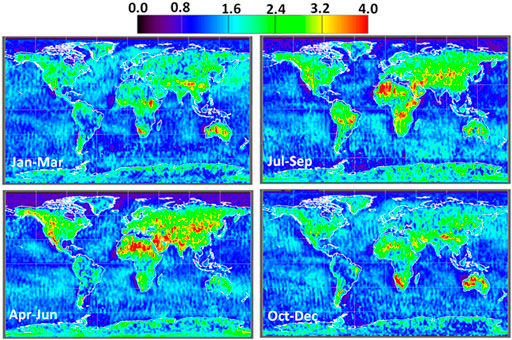
FIGURE 6. Average PBL height derived from application of the threshold algorithm to ICESat-2 data spanning all of 2019 and displayed in 3 month segments for a grid resolution of 2 × 2 degree.

Figure 7 displays the MERRA-2 reanalysis PBLH valid at 14:00 local time for each point on the globe. A local time of 14:00 was chosen because it corresponds to the maximum PBL height for most land areas and is likely to be best correlated with the lidar retrievals (at night over land, the lidar senses mainly the residual layer from the day before). The time of comparison over ocean does not matter due to the much smaller diurnal response of maritime PBLH. Over ocean, the MERRA-2 PBLH are considerably lower on average (800 m) than those of ICESat-2 (1,200 m) but exhibit similar patterns and seasonal differences as the ICESat-2 PBLH. For instance, east of continents over ocean the MERRA-2 PBL heights are higher in the winter hemisphere where cold air is advected from the land causing higher heat flux over the warmer water. MERRA-2 and ICESat-2 also exhibit lower PBLH off the west coast of major continents, due mainly to the upwelling of cold ocean water. The general pattern of the two oceanic PBLH agree, with areas of higher MERRA-2 PBLH corresponding to areas of higher ICESat-2 PBLH. Figure 8 displays only the maritime PBLH for both ICESat-2 and MERRA-2, but with a difference in data scaling so that the PBLH patterns are more discernable. Throughout most of the ocean, areas of higher and lower PBLH correspond. Ding et al. (2021) also found similar patterns and a low-bias in the MERRA-2 PBLH over oceans when comparing the MERRA-2 data to AIRS and COSMIC Radio Occultation estimates of PBLH.

FIGURE 7

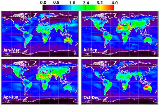
FIGURE 7. MERRA-2 PBL height at 14:00 local time for each quarter of 2019.

FIGURE 8

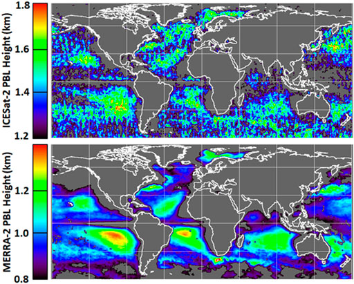
FIGURE 8. 2019 oceanic PBL height for ICESat-2 (top) and MERRA-2 (bottom). Note that each are scaled differently to bring out the correlation between the two PBLH results.

Over most of the land surface the MERRA-2 PBLH agrees well with ICESat-2, with notable exceptions being Antarctica, Greenland and northern high latitudes in winter. However, even in summer the MERRA-2 data show a marked decrease of PBLH north of about 58° latitude, which is not evident in the ICESat-2 retrievals. A PDF of MERRA-2 and ICESat-2 PBLH for 2019 is shown in Figure 9. The shape and widths of the ocean PDF (dashed) are similar, but the ICESat-2 peak is near 1,250 m whereas for MERRA-2 it is about 900 m. The land PDFs are similar for PBLH greater than about 2 km, but markedly different for PBLH less than that. The MERRA-2 peak for land occurs near 700 m with a considerable number of smaller heights. These are likely the mid and high latitude winter PBL heights and summer high latitude heights. The lower solar angle producing less daytime land heating is the probable cause of these low model PBL heights. The ICESat-2 land PBLH do not show this seasonal high latitude effect and the distribution is shifted to higher PBLH values (average of about 1800 m over land). These differences are probably due to the smaller high latitude daytime heating that will obviously reduce convective turbulence thereby leading to lower MERRA-2 PBLH. It is not known why the lidar-retrieved PBLH does not show this effect and a separate study would be required to understand these differences more fully. We have included maps of ICESat-2 minus MERRA-2 PBL height in Supplementary Figure S2. These show large areas of the ocean where the comparison agrees to within 100–200 m but most land areas have considerable disagreement. Also included in Supplementary Figure S1 are the percentage of time the 2019 ICESat-2 PBLH retrievals were made for each 1 × 1 degree grid box. This is computed as the number of successful PBLH retrievals made divided by the number of times that profiles were examined within a given grid box times 100.

FIGURE 9

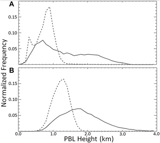
FIGURE 9. (A) MERRA-2 ocean (dashed) and land (solid) PBL height normalized probability distribution for 14:00 local time, January–December 2019. (B) Same as (A) except for all ICESat-2 PBLH data.

Convolutional Neural Network Algorithm

The convolutional neural network (CNN) algorithm explained in Convolutional Neural Network Method was applied to CATS nighttime data from 2016 and the resulting PBLH retrieval is shown in Figure 10A. For comparison, the results of the threshold algorithm applied to the same dataset are shown in Figure 10B. Recall that the CNN algorithm is trained using results from the threshold algorithm but has the distinct advantage in that it can work with uncalibrated backscatter data and it can achieve much higher horizontal resolution results. In fact, at least for nighttime data, the CNN algorithm can retrieve PBLH at the resolution of the acquired data (350 m for CATS). We show only nighttime granules because the solar background noise inherent in full resolution daytime granules causes a problem with the CNN technique. De-noising or horizontal averaging of the data will be required to achieve satisfactory results for daytime data. This is an area we are actively working on and hope to achieve reliable results for daytime data in the near future. We also plan to apply the CNN technique to ICESat-2 data once the daytime noise issues have been resolved.

FIGURE 10

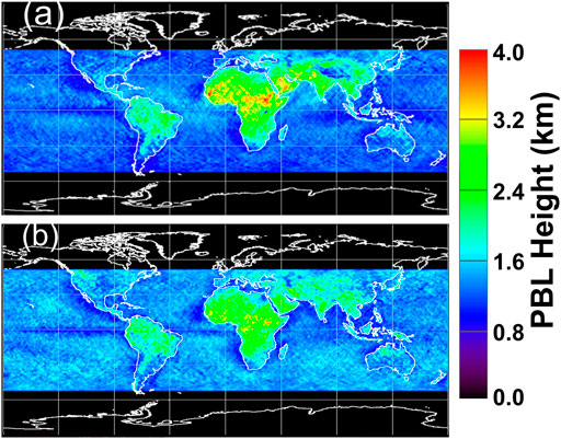
FIGURE 10. Average PBL height derived from the analysis of all CATS 2016 night granules using the CNN algorithm (A) and threshold algorithm (B).

Referring to Figure 10, there are several notable similarities and differences between the CATS PBLH using the two techniques. The magnitude and patterns of the PBLH over land are very similar, especially over the African continent, Middle East, India, and parts of South America and Southeast Asia. These are regions that typically experience higher aerosol loading and thus more accurate detection of PBLH (or nighttime residual layer height in many cases) using the threshold technique. However, the CNN technique appears to be lower than the threshold technique (for both CATS and ICESat-2) in areas of high terrain, such as the Rocky Mountains (western US), Himalayas, and Andes Mountains. Furthermore, the CNN technique has lower PBL heights in the northern latitudes over land, more comparable to the MERRA-2 results in Figure 7 than the threshold technique using ICESat-2 and CATS data. One possible explanation for this would be the ability of the CNN technique to detect more accurate cloud top heights due to its finer resolution, as shown in Figure 1. Over ocean, the CNN PBLH are lower than the threshold algorithm values with averages of 1.26 and 1.40 km, respectively.

In Figure 11 we show the comparison between MERRA-2 PBL height at 14:00 local time (upper four panels) and the average CNN PBL height derived from all CATS nighttime granules (lower 4 panels) for 3 month segments during 2016. Here we are showing only the MERRA-2 PBL height between 51S and 51N latitude, which roughly corresponds to the latitudinal limits of the ISS orbit. The CNN PBL height patterns over ocean are similar though they are about 300 m higher on average than MERRA-2. The CNN marine PBL heights show the higher PBLH east of major continents in the winter hemisphere and the lower marine PBL heights in the summer hemisphere, which is consistent with MERRA-2 and was also noted in the 2019 ICESat-2 results (Figure 6). The CNN and MERRA-2 PBL height values and patterns over land are generally consistent. However, notable differences exist mainly over the western U.S. and Australia where CNN PBL height is considerably lower than MERRA-2. It is not clear why this is so, though it may be related to the fact that only night granules are used in the CNN analysis. The 2019 ICESat-2 seasonal retrievals shown in Figure 6 (which used day and night data) do not show these low PBL height values in those regions. Also notable are lower CNN PBLH over northern Asia that agree better with MERRA-2 than did the threshold technique applied to 2019 ICESat-2 data.

FIGURE 11

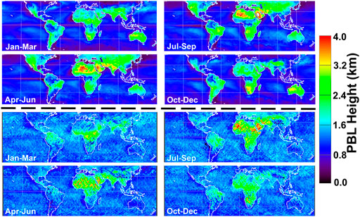
FIGURE 11. MERRA-2 2016 seasonal plots of PBL height at 14:00 local time (upper 4 plots) between 51S and 51N latitude and CATS average seasonal PBL height derived from all 2016 nighttime granules using the CNN algorithm (lower 4 plots).

Figure 12 shows the CATS 2016 PDFs comparing the CNN (dashed) and threshold algorithm (solid) PBL height over land (a) and ocean (b). Over land the peaks occur at 1.35 and 1.5 km and the average PBLH is 1.90 and 1.83 for CNN and threshold algorithms, respectively. Over ocean the peaks of the distributions are slightly lower than over land (1.2 and 1.3 km) and the average PBLH is 1.26 and 1.40 km for CNN and threshold algorithms, respectively. The widths of the ocean distributions are considerably narrower than for over land, which is consistent with the much lower variability of PBLH over ocean compared to land. We believe the lower CNN PBLH values for both land and ocean compared to the threshold results are due to the horizontal averaging employed by the threshold technique. Averaging the data over relatively large horizontal distance will tend to smear out the resulting backscatter profile (in the vertical) and just a few penetrating cumulus clouds that have reached higher than most will lead to a higher PBL height from the threshold technique. Conversely, the CNN method operates with no horizontal averaging and, while the CNN algorithm will return higher PBL height for these penetrating convective cells, they will be compensated by many other lower PBL heights between such cells.

FIGURE 12

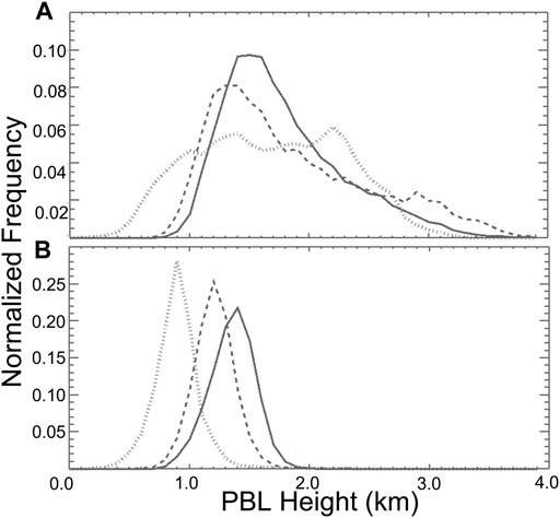
FIGURE 12. Normalized probability distributions of PBL height for land (A) and ocean (B) for all 2016 night CATS granules. The solid, dashed, and hatched lines correspond to results from the threshold and CNN algorithms and MERRA-2 reanalysis (14:00 Local time) between 51S and 51N, respectively.

Also shown in Figure 12 is a PDF of the 2016 MERRA-2 PBL heights at 14:00 local time for data between 51S and 51N latitudes (hatched line) for land (a) and ocean (b). The PDF of MERRA-2 PBL heights over land lack an obvious peak and are broader than those of either the CNN or threshold algorithm results. This might be due to a greater variability of observed atmospheric conditions in the MERRA-2 reanalysis. The average MERRA-2 land PBL height is 1.7 km compared to 1.90 and 1.83 for CNN and threshold algorithms, respectively. The shape of the MERRA-2 ocean PDF is similar to the CNN and threshold algorithm results, but is slightly more narrow, and shifted toward lower PBL heights. The median PBLH values for MERRA-2, CNN and threshold techniques over ocean are 0.9, 1.2 and 1.4 km, respectively.

Summary and Conclusion

In this work we have demonstrated the ability to retrieve PBL height from ICESat-2 and CATS backscatter lidar data on a global scale. Two techniques were presented, the first of which, called the threshold method, sets a backscatter threshold value based on the average calibrated, attenuated backscatter between 200 and 400 m above the surface of horizontally averaged profiles (64 km for daytime data, 24 km for night). The averaged profile is then searched upward from 400 m above the surface to a maximum altitude of 7 km (4 km over ocean) for two consecutive bins that fall below the determined threshold. If found, the first bin of which is set as the coarse height of the PBL. The profiles comprising the horizontal average are themselves analyzed at a higher resolution and in a narrow window around the coarse PBL height to obtain a finer (8x) horizontal resolution PBL height. Two case studies were presented that compared the threshold PBL height retrievals with nearly coincident (in space and time) radiosonde temperature and moisture profiles and showed good agreement with the conventional temperature inversion/moisture decrease definition of PBL top. The threshold algorithm was also applied to ICESat-2 data from 2019 and CATS data from 2016. The 2019 PBL height retrievals were compared with those from the MERRA-2 reanalysis and displayed a high degree of spatial correlation with the model heights but were about 400 m higher on average over ocean and over a km higher in northern hemisphere high latitude regions. The ocean results are consistent with McGrath-Spangler and Denning, (2012), who found that CALIPSO PBL height retrievals were higher over ocean than the MERRA-2 reanalysis. Over Africa, South America and Australia, the PBL heights agreed fairly well but the ICESat-2 heights were often 200–400 m lower than the MERRA-2 heights.

The second technique is based on a machine learning method known as a Convolutional Neural Network (CNN). This technique requires an extensive training dataset, and a month of PBL heights determined from the threshold method was used for this purpose. The distinct advantage of the CNN method is that it can work with raw, uncalibrated data and provide a much finer horizontal resolution. The CNN algorithm was applied to CATS 2016 nighttime raw (uncalibrated) data at full horizontal resolution (350 m) and showed very robust PBL height retrieval that agreed well with the threshold technique in some cases, but also diverged from it in others. These discrepancies were probably due to the horizontal averaging required by the threshold technique, and it is likely that the CNN result is better in these cases. Overall, compared to the threshold algorithm, the CNN technique produced somewhat lower (∼200 m) PBL height over the oceans and over mountainous and high latitude land areas. The CNN results were compared with MERRA-2 PBL height at 14:00 local time for 2016. As with the 2019 ICESat-2 comparison, the CNN results had a high spatial correlation with MERRA-2 over ocean but were on average about 300 m higher. Over land, notable discrepancies were over the western U.S. and Australia, where CNN PBLH were considerably lower than MERRA-2. However, over high northern latitude land masses, the CNN technique produced lower PBLH that better agree with MERRA-2 than the 2019 threshold technique comparison over this region.

Though the MERRA-2 reanalysis PBL heights shown in this study varied considerably from those derived from the satellite lidar data, one must remember that the definition of PBL height used by MERRA-2 is very different than that used to define PBL height from lidar backscatter profiles. PBL height from lidar is based on finding the height where a large gradient of scattering occurs, which is typically more aligned with the base of the capping temperature inversion. Models use varying definitions of PBL top and the MERRA-2 definition used here is based on the turbulent diffusion coefficient, which is obviously quite different. Because of this, the two cannot expect to agree exactly but the general spatial patterns should be similar and this has been seen in much of the data shown here.

In conclusion, satellite lidars like those presented here can provide useful information on planetary boundary layer height on a global scale. However, satellite lidars have their limitations, such as the inability to detect the PBL through attenuating clouds, daytime noise impacting horizontal resolution and accuracy, and sparse spatial coverage. This work demonstrates what a simple, single channel backscatter satellite lidar can accomplish for PBL height detection. Further, it shows that machine learning algorithms have the potential of increasing the accuracy and resolution of PBL height detection from space. With improvements to the algorithms presented here, such as differentiation between the nighttime stable and residual layers, and better daytime performance, future backscatter lidar instruments can provide a critical role in future PBL observing systems.

Data Availability Statement

Publicly available datasets were analyzed in this study. This data can be found here: The ICESat-2 calibrated attenuated backscatter data used to retrieve PBL height in this paper are freely available at the National Snow and Ice Data Center (NSIDC) via data product ATL09. Visit https://nsidc.org/data/icesat-2/data-sets to obtain the ICESat-2 atmospheric data products and documentation. The CATS data are publicly available from the NASA Langley Atmospheric Science Data Center (ASDC) at https://earthdata.nasa.gov/eosdis/daacs/asdc. All data product files are in hdf5 format.

Author Contributions

SP: lead author, wrote paper, developed threshold algorithm, ran it on ICESat-2 and CATS data and generated all figures 3-12 and supplemental figures. PS: second author, developed machine learning code, used threshold algorithm output to teach the Convolutional Neural Network (CNN), and generated figures 1 and 2. JY: third author, wrote CATS section of paper and helped to write CNN section. SN: fourth author, reviewed paper, made suggestions on content and form. EN: fifth author, obtained MERRA-2 data, checked accuracy of derived figures and edited paper.

Funding

This work was funded by the NASA Earth Science Technology Office (ESTO).

Conflict of Interest

Author SP is employed by Science Systems and Applications, Inc.

The remaining authors declare that the research was conducted in the absence of any commercial or financial relationships that could be construed as a potential conflict of interest.

Publisher’s Note

All claims expressed in this article are solely those of the authors and do not necessarily represent those of their affiliated organizations, or those of the publisher, the editors and the reviewers. Any product that may be evaluated in this article, or claim that may be made by its manufacturer, is not guaranteed or endorsed by the publisher.

Acknowledgments

The authors would like to thank the NASA Earth Science Technology Office for funding the work contained in this paper. Thanks also to the ICESat-2 project office and members of the ATLAS Science Algorithm Software (ASAS) development team who create the software to produce the ICESat-2 atmospheric data products. Thanks also to the ICESat-2 Science Investigator-led Processing System (SIPS) team that produce the actual data products and the ATLAS Instrument Support Team that manages flight operation of the ATLAS instrument.

Supplementary Material

The Supplementary Material for this article can be found online at: https://www.frontiersin.org/articles/10.3389/frsen.2021.716951/full#supplementary-material

Supplementary Figure S1 | For each 3 month period of 2019, the percentage of time the 2019 ICESat-2 PBLH retrievals were made for each 1 × 1 degree grid box. This is computed as the number of PBLH retrievals made divided by the number of times that data averages are made within a given grid box times 100. Rectangular areas that have very low retrieval rates are due to ICESat-2 calibrations during which no atmosphere data is collected (most evident in the Jan – Mar plot).

Supplementary Figure S2 | For each 3 month period of 2019, the difference between ICESat-2 average PBLH retrievals and MERRA-2 PBL height at 14:00 local time. The differences are shown in km and computed and shown on a 1 × 1 degree grid.

References

Abdalati, W., Zwally, H. J., Bindschadler, R., Csatho, B., Farrell, S. L., Fricker, H. A., et al. (2010). The ICESat-2 Laser Altimetry Mission. Proc. IEEE 98 (5), 735–751. doi:10.1109/JPROC.2009.2034765

CrossRef Full Text | Google Scholar

Abshire, J. B., Sun, X., Riris, H., Sirota, J. M., McGarry, J. F., Palm, S., et al. (2005). Geoscience Laser Altimeter System (GLAS) on the ICESat Mission: On-Orbit Measurement Performance. Geophys. Res. Lett. 32, L21S02. doi:10.1029/2005GL024028

CrossRef Full Text | Google Scholar

Bosart, L. F. (1981). The Presidents' Day Snowstorm of 18-19 February 1979: A Subsynoptic-Scale Event. Mon. Wea. Rev. 109, 1542–1566. doi:10.1175/1520-0493(1981)109<1542:tpdsof>2.0.co;2

CrossRef Full Text | Google Scholar

Chepfer, H., Brogniez, H., and Noel, V. (2019). Diurnal Variations of Cloud and Relative Humidity Profiles across the Tropics. Sci. Rep. 9, 16045. doi:10.1038/s41598-019-52437-6

PubMed Abstract | CrossRef Full Text | Google Scholar

Christian, K., Wang, J., Ge, C., Peterson, D., Hyer, E., Yorks, J., et al. (2019). Radiative Forcing and Stratospheric Warming of Pyrocumulonimbus Smoke Aerosols: First Modeling Results with Multisensor (EPIC, CALIPSO, and CATS) Views from Space. Geophys. Res. Lett. 46 (10), 10071–10061. 071. doi:10.1029/2019GL082360

CrossRef Full Text | Google Scholar

Cohn, S. A., and Angevine, W. M. (2000). Boundary Layer Height and Entrainment Zone Thickness Measured by Lidars and Wind-Profiling Radars. J. Appl. Meteorol. 39, 1233–1247. doi:10.1175/1520-0450(2000)039%3C1233:BLHAEZ%3E2.0.CO;2

CrossRef Full Text | Google Scholar

Davis, K. J., Lenschow, D. H., Oncley, S. P., Kiemle, C., Ehret, G., and Giez, A. (1997). Role of Entrainment in Surface–Atmosphere Interactions over the Boreal forest. J. Geophys. Res. 102, 29 219–229 230.

CrossRef Full Text | Google Scholar

Ding, F., Iredall, L., Theobald, M., Wei, J., and Meyer, D. (2021). PBL Height from AIRS, GPS RO, and MERRA-2 Products in NASA GES 1 DISC and Their 10-Year Seasonal Mean Intercomparison. Earth Space Sci.. doi:10.1029/2021ea001859

CrossRef Full Text | Google Scholar

Gidaris, S., and Komodakis, N. (2015). “Object Detection via a Multi-Region and Semantic Segmentation-Aware CNN Model,” in The IEEE International Conference on Computer Vision (ICCV), Santiago, Chile, December 7–13, 2015 (IEEE), 1134–1142. doi:10.1109/iccv.2015.135

CrossRef Full Text | Google Scholar

Hughes, E. J., Yorks, J., Krotkov, N. A., da Silva, A. M., and McGill, M. (2016). Using CATS Near-Real-Time Lidar Observations to Monitor and Constrain Volcanic Sulfur Dioxide (SO2) Forecasts. Geophys. Res. Lett. 43, 11089–11097. doi:10.1002/2016GL070119

CrossRef Full Text | Google Scholar

Jordan, N. S., Hoff, R. M., and Bacmeister, J. T. (2010). Validation of Goddard Earth Observing System-Version 5 MERRA Planetary Boundary Layer Heights Using CALIPSO. J. Geophys. Res. 115, D24218. doi:10.1029/2009JD013777

CrossRef Full Text | Google Scholar

Lee, L., Zhang, J., Reid, J. S., and Yorks, J. E. (2019). Investigation of CATS Aerosol Products and Application toward Global Diurnal Variation of Aerosols. Atmos. Chem. Phys. 19, 12687–12707. doi:10.5194/acp-19-12687-2019

CrossRef Full Text | Google Scholar

Lewis, J. R., Welton, E. J., Molod, A. M., and Joseph, E. (2013). Improved Boundary Layer Depth Retrievals from MPLNET. J. Geophys. Res. Atmos. 118, 9870–9879. doi:10.1002/jgrd.50570

CrossRef Full Text | Google Scholar

Liu, J., Huang, J., Chen, B., Zhou, T., Yan, H., Jin, H., et al. (2015). Comparisons of PBL Heights Derived From CALIPSO and ECMWF Reanalysis Data Over China. J. Quant. Spectrosc. Ra. 153, 102–112.

CrossRef Full Text | Google Scholar

Maskey, M., Ramachandran, R., Miller, J. J., Zhang, J., and Gurung, I. (2018). “Earth Science Deep Learning: Applications and Lessons Learned,” in IGARSS 2018 - 2018 IEEE International Geoscience and Remote Sensing Symposium, Valencia, Spain, July 22–27, 2018. Available at: https://ntrs.nasa.gov/archive/nasa/casi.ntrs.nasa.gov/20180008578.pdf.

CrossRef Full Text | Google Scholar

McGill, M. J., Swap, R. J., Yorks, J. E., Selmer, P. A., and Piketh, S. J. (2020). Observation and Quantification of Aerosol Outflow from Southern Africa Using Spaceborne Lidar. S. Afr. J. Sci. 116 (3/4), 6398–6404. doi:10.17159/sajs.2020/6398

CrossRef Full Text | Google Scholar

McGill, M. J., Yorks, J. E., Scott, V. S., Kupchock, A. W., and Selmer, P. A. (2015). The Cloud-Aerosol Transport System (CATS): a Technology Demonstration on the International Space Station. Lidar Remote Sensing Environ. Monit. XV, 96120A. doi:10.1117/12.2190841

CrossRef Full Text | Google Scholar

McGrath-Spangler, E. L., and Denning, A. S. (2012). Estimates of North American Summertime Planetary Boundary Layer Depths Derived from Space-Borne Lidar. J. Geophys. Res. 117, a–n. doi:10.1029/2012JD017615

CrossRef Full Text | Google Scholar

McGrath-Spangler, E. L., and Denning, A. S. (2013). Global Seasonal Variations of Midday Planetary Boundary Layer Depth from CALIPSO Space-Borne Lidar. J. Geophys. Res. Atmos. 118, 1226–1233. doi:10.1002/jgrd.50198

CrossRef Full Text | Google Scholar

Melfi, S. H., Spinhirne, J. D., Chou, S.-H., and Palm, S. P. (1985). Lidar Observations of Vertically Organized Convection in the Planetary Boundary Layer over the Ocean. J. Clim. Appl. Meteorol. 24, 806–821. doi:10.1175/1520-0450(1985)024<0806:loovoc>2.0.co;2

CrossRef Full Text | Google Scholar

Noel, V., Chepfer, H., Chiriaco, M., and Yorks, J. (2018). The Diurnal Cycle of Cloud Profiles over Land and Ocean between 51° S and 51° N, Seen by the CATS Spaceborne Lidar from the International Space Station. Atmos. Chem. Phys.. doi:10.5194/acp-2018-214

CrossRef Full Text | Google Scholar

O'Sullivan, D., Marenco, F., Ryder, C. L., Pradhan, Y., Kipling, Z., Johnson, B., et al. (2020). Models Transport Saharan Dust Too Low in the Atmosphere: a Comparison of the MetUM and CAMS Forecasts with Observations. Atmos. Chem. Phys. 20, 12955–12982. doi:10.5194/acp-20-12955-2020

CrossRef Full Text | Google Scholar

Palm, S. P., Benedetti, A., and Spinhirne, J. (2005). Validation of ECMWF Global Forecast Model Parameters Using GLAS Atmospheric Channel Measurements. Geophys. Res. Lett. 32, a–n. doi:10.1029/2005GL023535

CrossRef Full Text | Google Scholar

Palm, S. P., Yang, Y., Herzfeld, U., Hancock, D., Hayes, A., Selmer, P., et al. (2021). Review.ICESat-2 Atmospheric Channel Description, Data Processing and First Results. Earth Space Sci.

Google Scholar

Palm, S. P., Yang, Y., and Herzfeld, U. (2020): Ice, Cloud, and Land Elevation Satellite (ICESat-2) Project Algorithm Theoretical Basis Document for the Atmosphere, Part I: Level 2 and 3 Data Products, version 3 doi:10.5067/X6N528CVA8S9

CrossRef Full Text | Google Scholar

Pauly, R. M., Yorks, J. E., Hlavka, D. L., McGill, M. J., Amiridis, V., Palm, S. P., et al. (2019). Cloud-Aerosol Transport System (CATS) 1064 Nm Calibration and Validation. Atmos. Meas. Tech. 12, 6241–6258. doi:10.5194/amt-12-6241-2019

PubMed Abstract | CrossRef Full Text | Google Scholar

Pradhan, R., Aygun, R. S., Maskey, M., Ramachandran, R., and Cecil, D. J. (20182018). Tropical Cyclone Intensity Estimation Using a Deep Convolutional Neural Network. IEEE Trans. Image Process. 27 (2), 692–702. doi:10.1109/tip.2017.2766358

PubMed Abstract | CrossRef Full Text | Google Scholar

Rajapakshe, C., Zhang, Z., Yorks, J. E., Yu, H., Tan, Q., Meyer, K., et al. (2017). Seasonally Transported Aerosol Layers over Southeast Atlantic Are Closer to Underlying Clouds Than Previously Reported. Geophys. Res. Lett. 44, 5818–5825. doi:10.1002/2017GL073559

PubMed Abstract | CrossRef Full Text | Google Scholar

Rienecker, M. M. (2008). “The GEOS‐5 Data Assimilation System— Documentation of Versions 5.0.1 and 5.1.0,” in NASA GSFC Technical Report Series on Global Modeling and Data Assimilation (Greenbelt, MD: NASA tech memo at Goddard Space Flight Center), 27, 92.

Google Scholar

Shahin, M. A., Maier, H. R., and Jaksa, M. B. (2004). Data Division for Developing Neural Networks Applied to Geotechnical Engineering. J. Comput. Civ. Eng. 18, 105–114. doi:10.1061/(asce)0887-3801(2004)18:2(105)

CrossRef Full Text | Google Scholar

Spinhirne, J. D., Palm, S. P., Hart, W. D., Hlavka, D. L., and Welton, E. J. (2005). Cloud and Aerosol Measurements from GLAS: Overview and Initial Results. Geophys. Res. Lett. 32, a–n. doi:10.1029/2005GL023507

CrossRef Full Text | Google Scholar

Stull, R. B. (1988). An Introduction to Boundary Layer Meteorology. Norwell, Mass: Kluwer Acad., 666.

Teixeira, J., Piepmeier, J. R., Nehrir, A. R., Ao, C. O., Chen, S. S., Clayson, C. A., et al. (2021). Toward a Global Planetary Boundary Layer Observing System: The NASA PBL Incubation Study Team Report. Washington, DC: NASA PBL Incubation Study Team, 134 https://science.nasa.gov/science-pink/s3fs-public/atoms/files/NASAPBLIncubationFinalReport.pdf.

Tracton, M. S. (1973). The Role of Cumulus Convection in the Development of Extratropical Cyclones. Mon. Wea. Rev. 101, 573–593. doi:10.1175/1520-0493(1973)101<0573:trocci>2.3.co;2

CrossRef Full Text | Google Scholar

Van Pul, W. A. J., Holtslag, A. A. M., and Swart, D. P. J. (1994). A Comparison of ABL Heights Inferred Routinely from Lidar and Radiosondes at Noontime. Boundary-layer Meteorol. 68, 173–191. doi:10.1007/bf00712670

CrossRef Full Text | Google Scholar

Yorks, J. E., McGill, M. J., Palm, S. P., Hlavka, D. L., Selmer, P. A., Nowottnick, E. P., et al. (2016). An Overview of the CATS Level 1 Processing Algorithms and Data Products. Geophys. Res. Lett. 43, 4632–4639. doi:10.1002/2016GL068006

CrossRef Full Text | Google Scholar

Yorks, J. E., Selmer, P. A., Kupchock, A., Nowottnick, E. P., Christian, K. E., Rusinek, D., et al. (2021). Aerosol and Cloud Detection Using Machine Learning Algorithms and Space-Based Lidar. Atmosphere 12, 606. doi:10.3390/atmos12050606

CrossRef Full Text | Google Scholar

Yu, Y., Kalashnikova, O. V., Garay, M. J., Lee, H., Choi, M., Okin, G. S., et al. (2021). A Global Analysis of Diurnal Variability in Dust and Dust Mixture Using CATS Observations. Atmos. Chem. Phys. 21, 1427–1447. doi:10.5194/acp-21-1427-2021

CrossRef Full Text | Google Scholar