Radiative Transfer Speed-Up Combining Optimal Spectral Sampling With a Machine Learning Approach

1 Introduction

Carbon dioxide (CO₂) is one of the primary greenhouse gases in Earth’s atmosphere. To better understand its sources and sinks in the carbon cycle, the Orbiting Carbon Observatories-2 (OCO-2) (Eldering et al., 2017) and -3 (OCO-3) (Eldering et al., 2019) make space-based measurements of reflected sunlight to retrieve column averaged CO₂ dry mole factions (X_CO2). When sunlight passes through the atmosphere, a wavelength-dependent fraction gets absorbed. How much sunlight gets absorbed depends on, besides other factors, the concentration of various atmospheric gases, such as oxygen (O₂), CO₂, water vapor (H₂O), and carbon monoxide (CO), as well as on the concentration of aerosol and cloud particles which modulate photon path length. The OCO-2/3 sensors have three instrument channels to measure reflected sunlight at a high spectral resolution in the oxygen A-band (O2A-band) as well as the weak and strong CO2-bands (WCO2-band and SCO2-band), located at 0.76, 1.61, and 2.06 µm, respectively. To derive X_CO2 from these measurements, OCO-2/3 employs an optimal estimation (OE) retrieval algorithm, termed as the ACOS retrieval (C. O'Dell et al., 2018). The ACOS retrieval employs a physics-based retrieval with uncertainty quantification. In an iterative process, a physical radiative transfer forward model (Bösch et al., 2006; Connor et al., 2008; O'Dell et al., 2018; O'Dell et al., 2012) is used to calculate the top-of-atmosphere radiances from a state vector that is defined a priori. This modeled radiance is then compared to the measured radiance observed by OCO-2/3. Next, differences between the calculated and measured spectrum are propagated back to the forward model and a new spectrum is computed with an updated state vector. The process is repeated until a minimum error threshold between measured and calculated radiances is reached or the maximum number of iterations is exceeded. Besides many other variables, the final state vector provides an estimate of X_CO2. To keep the error in the retrieved X_CO2 below 0.1%, the error in the forward radiative transfer model (RTM) needs to be itself on the order of no more than 0.1% (Hasekamp & Butz, 2008). This places strict accuracy requirements on any RTM. Such accuracy can be achieved with computationally expensive high-resolution calculations that take the spectrally varying absorption of gases into consideration [e.g., LBLRTM (Clough et al., 2005)]. However, OCO-2 produces 1 million soundings every day which yields approximately 100,000 cloud-free soundings. This results in 40 million cloud-free soundings per year that need to be processed. Retrieving X_CO2 from these soundings requires running OE and the RTM for each sounding multiple times. As the mission gets longer, reprocessing time and cost increases for new releases to the point that it might become too expensive to reprocess the data altogether. Most of the time spent during OE is spent in the RTM, approximately 92%. This work describes the latest developments by the OCO-2 mission to reduce the computational cost of these calculations. Besides OCO-2 and OCO-3, the developed approach can be readily applied to other greenhouse gas sensors such as GeoCarb (Moore et al., 2018), CO2M (Kuhlmann et al., 2019), and hyperspectral instruments in general that operate from the ultra violet to the shortwave infrared.

1.1 Radiative Transfer Speed-Up Methods

The computational cost of high-resolution calculations has been a bottleneck for many applications over the last few decades. A variety of methods have been developed to ease the computational burden. For example, the correlated-k method (Goody et al., 1989; Lacis and Oinas, 1991) is frequently used to speed up RTMs by dividing the spectrum into bands that can be described by a small number of coefficients and weights. Using these coefficients, pseudo-monochromatic calculations are performed that can then be used to reconstruct the full spectrum. Building on correlated-k “exponential sum fitting” (Wiscombe and Evans, 1977) can be used to optimize the number of k values where the mean transmittance is expressed as the weighted sum of exponentials at monochromatic wavelengths. Similarly, optimal spectral sampling (OSS) (Moncet et al., 2015) expands upon exponential sum fitting by directly approximating radiances from a subset of monochromatic RTM calculations. The accuracy, with respect to line-by-line calculations can be tuned by the number of monochromatic wavelengths being used. Alternatively, principal components can be used to speed up RTMs (Natraj et al., 2005; Liu et al., 2006; Efremenko et al., 2014). Unfortunately, errors associated with most RTM speed-up approaches well exceed the targeted 0.1% error budget for OCO-2. More recently, the use of machine learning is gaining attention to further accelerate RTMs (Reichstein et al., 2019). Machine learning approaches can unfold their full potential if enough training data are available to fit the model. Fortunately, to replace an RTM with a machine learning approach, the RTM itself can be used to generate a training data set, theoretically of any size. There exist end-to-end approaches where the radiances are directly modeled from the state vector with more complex machine learning models such as neural networks (Bue et al., 2019; Pal, Mahajan, & Norman, 2019; Gao et al., 2021; Brence et al., 2022) or Gaussian processes (Gómez-Dans et al., 2016; Vicent et al., 2018; Svendsen et al., 2020). End-to-end approaches can be multiple orders of magnitude faster than more traditional approaches since they omit the costly RTM calculations entirely. However, end-to-end approach struggles with high-accuracy requirements for high-dimensional state spaces. Additionally, approaches using neural networks have the inherent shortcoming of being less interpretable than other methods and can exhibit erroneous non-linear behavior when extrapolating from the state space they were trained on. This can lead to large unexpected errors. Other approaches to accelerate RTMs with the help of machine learning replace only part of a RTM. These methods are often referred to as hybrid approaches and merge calculations based in physics and statistical methods. For example, low-fidelity physical radiative transfer calculations can be augmented by a neural network to match those of high-fidelity calculations (Brodrick et al., 2021), radiative transfer calculations performed at a subset of wavelengths can be extended across the entire spectral range (Le et al., 2020), or a neural network is used to predict the atmospheric transmittance profile that can then be used in a physical RTM (Stegmann et al., 2022). Using a hybrid approach reduces the dimensionality of the challenge compared to end-to-end approaches at the cost of an increased computational burden.

Finally, there is the approach currently implemented in the operational OCO-2 processing pipeline. This approach relies on a 2-step RTM. First, a fast low-accuracy 2-stream RTM that is used to calculate a spectrum given a state vector. In the second step, this low-accuracy spectrum is “adjusted” with a small number of high-accuracy RTM calculations that account for multiple scattering by using 24 streams (Christopher W O'Dell, 2010). The wavelengths at which the high-accuracy calculations are performed are selected so that they evenly sample the column-integrated gas optical depth as well as a multiple scattering error term, further described in Duan et al. (2005). This effectively reduces the computational cost by orders of magnitude compared to high-accuracy calculations over the full spectral range. Additionally, to further speed-up the calculations, the low-accuracy calculations are performed only at a subset of wavelengths with the remaining wavelengths being filled in by linear interpolation. This interpolation step reduces the number of required low-accuracy RTM calculations to approximately 8,000 in the O2A-band and SCO2-band, respectively, and 3,000 in the WCO2-band. This reduces the computational cost of the low-accuracy calculations by an additional ∼60%.

Nevertheless, the forward model is still a significant bottleneck in OCO-2/3’s OE retrieval. Reprocessing the full data record for new versions requires a significant financial investment as well as more than a year of reprocessing time. This results in a significant delay between updates made to the RTM and providing new data to the community that benefits from those updates. Therefore, we investigated how an additional algorithm speed-up could be realized while maintaining most of the existing and validated algorithm. A prime candidate for additional speed-up of the RTM is the high level of correlation within the low-accuracy calculations. The current linear interpolation exploits the correlation at neighboring wavelengths but does not utilize the correlation of non-neighboring wavelengths. We experimented with linear and non-linear machine learning approaches (linear regression, random forests, and neural networks) aiming for a method that would provide a significant benefit over the current approach. Using some initial experiments, we down selected the possible approaches to a model that exploits non-neighboring correlations in a simple and fully interpretable manner that is described in the following.

The structure of this article is as follows: in Section 2, we discuss the data set used in this study, Section 3 details how we model spectra from a subset of wavelengths, Section 4 discusses the results followed by discussion in Section 5. Finally, Section 6 provides a conclusion and discusses next steps.

2 Data Characteristics

We selected a subset of the OCO-2 data record by sampling every fourth land nadir and ocean glint sounding from days 1, 6, 11, 17, 22, and 27 from each month between January 2016 and March 2017. Cloudy scenes were excluded since they are flagged and removed in a preprocessing step before the operational OE retrieval. This results in a set of 20,948 OCO-2 soundings that are used in this study. For each sounding, we performed the RTM calculations on the high-resolution (0.01 cm⁻¹) for the at-sensor reflectance over the full spectral range of the three OCO-2 instrument bands. For the O2A-band, WCO2-band, and SCO2-band the high-resolution grid has 27,494, 12,961, and 10,690 points, respectively. The distribution of the soundings over various state variables is shown in Figure 1.

FIGURE 1

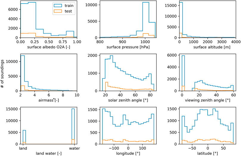
FIGURE 1. Distribution of subset of state variables from OCO-2 soundings used in this study. Training set is shown in blue, Testing set in orange. *Airmass describes the relative airmass of a sounding defined as 1/cos (solar zenith angle) + 1/cos (viewing zenith angle).

The soundings were split into a training, validation, and testing set. Each set consists of a subset of the considered soundings that are exclusive to this set. To avoid data leakage between the three data sets, we split the soundings by their observation time, with the first 80% of soundings (01/01/2016 to 12/27/2017) being used for the training set, the next 10% (01/01/2017 to 02/11/2017) being used for the validation set, and the remaining 10% (02/17/2017 to 03/27/2017) for the testing set. The training set was used to fit the model parameters, or train the model; the validation set was used to estimate how well the model generalizes to new data and tune various model parameters; and the testing set to report the final model accuracy.

2.1 Dimensionality

While OCO-2/3 samples each instrument band over 1,016 wavelength bins, the unconvolved calculated spectra require roughly an order of magnitude more monochromatic radiance calculations to accurately capture the underlying spectral features. The radiances at these wavelengths are not independent and, in part, governed by the same physical processes, for example, the absorption by oxygen or the scattering by aerosols. To estimate the degrees of freedom of each instrument band, we performed a principal component analysis (PCA) using the training set and investigated how many principal components (PC) are required to describe 99.9% of the variability in each band.

The cumulative explained variance for the first 15 PCs (variance of the original signal that can be described by the combination of the first 15 PCs) of the O2A-band, WCO2-band, and SCO2-band is shown in Figure 2. The WCO2-band has the lowest dimensionality with the first two PCs describing 99.9% of the variance. The O2A-band and SCO2-band require approximately four PCs to describe 99% of the variability and an additional five PCs to describe 99.9% of the variance. Note that these PCs are for simulated, monochromatic spectra with no Doppler shifts, instrument noise, or other instrumental effects. Given the more than 10,000 wavelengths of each channel, there seems to be a large degree of correlation within each band. Judging from the PCA, we expect the WCO2-band to require the least amount of information to be modeled and even though the O2A-band contains almost twice as many monochromatic wavelengths, we expect to require the same amount of information for this band as for the SCO2-band.

FIGURE 2

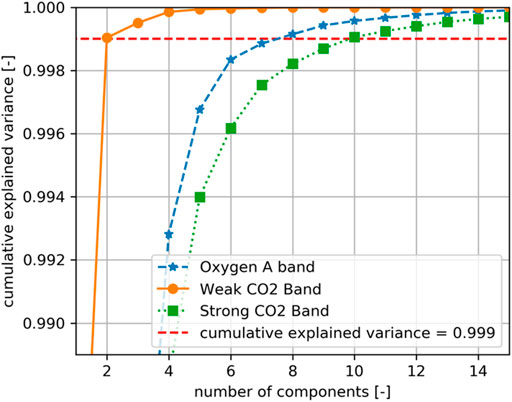
FIGURE 2. Cumulative explained variance of the first 15 principal components for the three OCO-2/3 instrument bands. O2A-band is shown with blue stars, WCO2-band with orange dots, and SCO2-band with green squares. Note, for clarity, cumulative explained variance is shown only from 0.99 to 1.0 and, therefore, omits data points that have a cumulative explained variance of less than 0.99.

3 Methods

3.1 Modeling Spectra From a Subset of Wavelengths

As a first order approximation, following Beer’s law (Swinehart, 1962), the monochromatic radiance measured by OCO-2/3, $I_{\lambda }$ [W·sr⁻¹·m⁻³], can be approximated by the incoming top-of-atmosphere solar radiance, $I_{\lambda \mathrm{s}\mathrm{u}\mathrm{n}}$, divided by the cosine of the solar zenith angle, $\mu$, multiplied by the surface albedo, $\rho$, and atmospheric transmittance which depends exponentially on airmass, m [-] and absorption optical depth, ${\tau }_{\lambda }$ (see Eq. 1). For the purposes of explanation, we assume a constant surface albedo across the band. This assumption easily generalized to a linear or quadratic dependence, as is used in the ACOS retrieval. Note, Eq. 1 does not account for emitted radiation from the surface or atmosphere. Thus, the proposed method is limited to applications where emitted radiation by the surface or atmosphere can be neglected.

To model the relationship between the radiance at individual wavelengths, we first take the natural logarithm of the radiance. This linearizes the relationship between wavelengths within a given instrument band. Afterwards, we can approximate the radiance at each wavelength of the full-resolution spectrum as a linear combination of the radiance at a subset of wavelengths, $\mathit{i}$, by multiplying them by matrix, $\mathit{A}$, from now on referred to as “correlation matrix.” Finally, we take the exponent of this product to get back to the predicted radiances, $\widehat{i}$ (see Eq. 2). For this relationship, $I_{\lambda \mathrm{s}\mathrm{u}\mathrm{n}}$ and $\rho$ can be omitted since they can be approximated as constant (variations in $I_{\lambda \mathrm{s}\mathrm{u}\mathrm{n}}$ are small compared to OCO-2/3 accuracy and the wavelengths dependence of $\rho$ can be neglected for the narrow OCO-2/3 bands).

$I_{\lambda }=\rho \frac{I_{\lambda \mathrm{s}\mathrm{u}\mathrm{n}}}{\mu } e^{-m{\tau }_{\lambda }},(1)$

$\widehat{\mathit{i}}=\mathrm{e}\mathrm{x}\mathrm{p}(\ln \left(\mathit{i}\right) \mathit{A}),(2)$

$cost=\alpha R\left(\mathit{A}\right)+\frac{1}{2n}{\displaystyle \sum }_{k=1}^n{\left({\widehat{\mathit{i}}}_k-{\mathit{i}}_l\right)}^2\mathrm{w}\mathrm{i}\mathrm{t}\mathrm{h}R\left(\mathit{A}\right)={\mathit{||A||}}_2={\displaystyle \sum }_{k,l=1}^n{\mathit{A}}_{k,l}^2.(3)$

For 800 input wavelengths, the correlation matrix, $\mathit{A}$, for the O2A-band, WCO2-band, and SCO2-band contains 800 rows and 27,494, 12,961, and 10,690 columns, respectively. This results in approximately 20 million free parameters for the O2A-band and 10 million parameters for the WCO2- and SCO2-band that need to be determined using the training set. Rather than solving for the correlation matrix directly we first initialize $\mathit{A}$ randomly and then minimizing the root mean square error between the reconstructed spectrum, $\widehat{\mathit{i}}$, and the true spectrum, $\mathit{i}$, for the set of trainings spectra (see Eq. 3). For the minimization, we use the Google TensorFlow framework (Abadi et al., 2016) and Adam gradient descent algorithm (Kingma & Ba, 2014). To make this iterative process robust, the radiance at each wavelength is standardized by subtracting the mean and dividing by the standard deviation as calculated from the training set. Additionally, we add L2 regularization (R(A) in Eq. 3), also referred to as weight decay, to our cost function with a small weighting factor of $\alpha$ = 1e-11. The L2 regularization helps to avoid overfitting to the training set by encouraging smaller values in the correlation matrix, $\mathit{A}$. The weighting factor, was determined empirically using the validation set.

Note the approximation we make in Eqs 1, 2 neglects various wavelength-dependent non-linear effects, such as rotational Raman scattering (Sioris & Evans, 2000) and small spectral dependencies by aerosols and surface albedo. Additionally, solar-induced fluorescence (SIF) (Sun et al., 2017) is not captured in our approximation. For OCO-2/3, SIF is calculated separately and added to the radiance calculations in a post-processing step. Thus, it is not considered for our approximation. Doppler shifts, the impact of the solar spectrum, and convolution with the instrument line shape function (ILS) all happen downstream of this algorithm in the forward model, and therefore need not be considered.

To summarize, each high-resolution spectrum is modeled from calculated monochromatic radiances at a subset of wavelengths. This approach is similar to the linear interpolation that is currently implemented operationally in the OCO-2/3 processing pipeline. However, the new approach allows to exploit not only the relationship of the radiance at neighboring wavelengths but of each wavelength to each other wavelength.

3.2 Finding the Most Informative Wavelengths

To identify which subset of wavelengths contains the most information to model the full resolution spectrum, we utilize an autoencoder. Autoencoders have been previously used for feature selection (Han et al., 2018) and allow considering linear as well as non-linear relationships between input wavelengths. An autoencoder consists of three pieces, an encoder, that projects the data into a lower dimensional space, a bottleneck, that constrains the dimensionality of the low-dimensional space, and a decoder that projects the data from the low-dimensional space back into its original form. To train the autoencoder, a loss function is minimized using gradient descent that measures the difference between the original spectrum and reconstructed spectrum after encoding and decoding. For our application, we used a neural network with 100 neurons in the layers that encode and decode the data, respectively. Initial experiments showed that more neurons in the encoder and decoder lead to similar results but at a higher computational cost. The middle layer that forms the bottleneck consists of 20 neurons. The number of neurons for the bottleneck were chosen as a tradeoff between being able to reconstruct the spectra with high accuracy and being able to order the importance of individual wavelengths down to only a few remaining wavelengths (once the number of wavelengths drop below the number of neurons in the bottleneck they cannot be sorted anymore). This architecture forces the neural network to encode the full high-resolution spectrum (∼27,000 wavelength for the O2A-band, ∼11,000 wavelengths for the weak and strong CO2-bands) into a 20-dimensional latent space and then reconstruct it from this space. This requires the neural network to weight the contribution of each wavelength to the 20-dimensional space. Wavelengths that contain redundant information will be given less weight while wavelengths that carry unique information will be given more weight. To extract this weighting, we applied the following approach to spectra of each instrument channel separately.

Using the training set we train the autoencoder for 100 epochs, then we randomly pick a set of 100 wavelengths, perturb each wavelength, and measure the mean square error (MSE) between the original and encoded and decoded spectra. The 10 wavelengths that have the least effect on the MSE are deemed the least important and removed. This process is repeated until only 20 wavelengths are left. The later a wavelength is removed, the higher this wavelength’s information content.

An alternative approach to find the most informative input wavelengths of each band is to calculate the pairwise correlation of all wavelengths and iteratively choose and remove wavelengths that are highly correlated. This has recently been proposed by Bai et al. (2020) and we compare our approach of using an auto-encoder to this method. Please refer to (Bai et al., 2020) for a detailed description of the algorithm.

4 Results

4.1 Informative Wavelengths

Figures 3A,B show the ordering of the wavelengths for the O2A-band as determined by the autoencoder from least to most informative. For the O2A-band, the most informative wavelengths are in the continuum at both ends of the band as well as deep in the absorption bands. This suggests that the degrees of freedom of the spectra in the O2A-band are constrained both by the reflected radiance at wavelengths where there is little to no absorption (information about solar and viewing geometry as well as aerosols and surface reflectance) as well as wavelengths with high gas absorption (abundance of various absorbing gases in the atmosphere, including CO₂). The optical properties of aerosols and the surface albedo are typically a smooth function of wavelength. For the narrow instrument bands for OCO-2/3, this allows to interpolate some of these characteristics. Similarly, the gas absorption at a given wavelength is dependent on the abundance of a certain gas. This abundance can be best approximated from the wavelengths that are deep in the absorption bands. Figures 3C,D show a similar plot but for the WCO2-band. Similar to the O2A-band the wavelengths in the continuum seem to carry the most information about the spectrum. Figures 3E,F show the most important wavelengths for the SCO2-band.

FIGURE 3

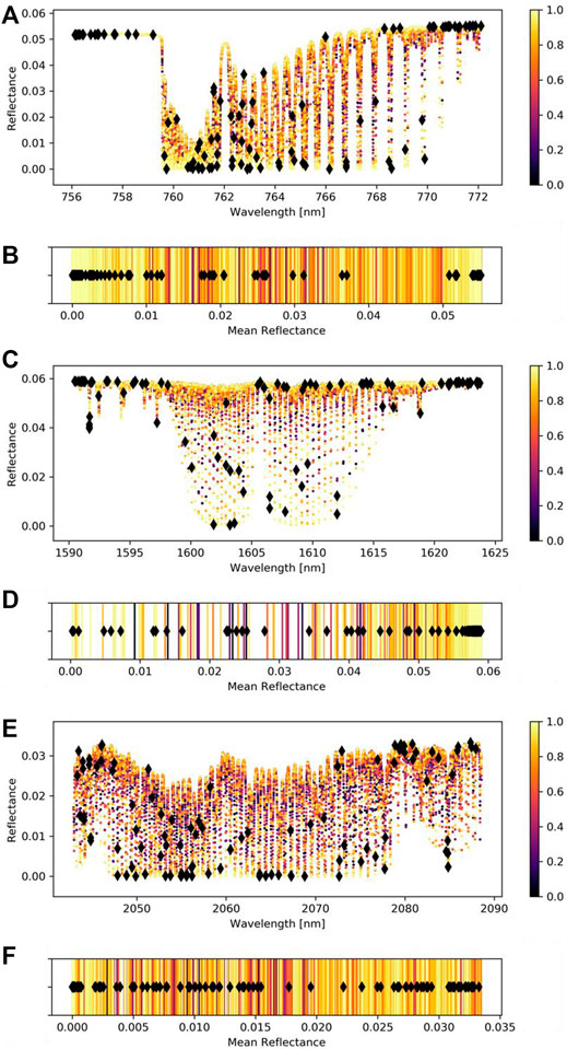
FIGURE 3. Ordering of information content of each wavelength as determined by the autoencoder for O2A-band (A,B), WCO2-band (C,D), and SCO2-band (E,F). The 100 most important wavelengths are highlighted with black diamonds. The most informative wavelengths are shown in yellow, the least informative wavelengths in black.

To better understand how the individual wavelengths contribute to the modeled spectra, we show the structure of the fit correlation matrix for each instrument channel in Figure 4. Positive entries are shown in red and indicate a positive correlation between input wavelengths and output wavelengths. Negative entries are shown in blue and indicate a negative correlation. For the O2A-band (Figure 4A), wavelengths in the continuum (756–759 nm) are clearly correlated with each other. The same is true at longer wavelengths (770–772 nm) where most but not all wavelengths are in the continuum as well. However, there seems to be little information that links the continuum from both sides of the O2A-band. For the WCO2-band (Figure 4B) and SCO2-band (Figure 4C), the structure of the correlation matrix is less pronounced. However, as one would expect, there seems to be a small increase in positive correlation for neighboring wavelengths, indicated by a red diagonal stripe around the one-to-one line.

FIGURE 4

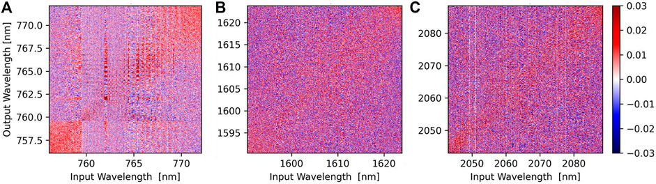
FIGURE 4. Correlation matrix, A, for the O2A-band (A), WCO2-band (B), and SCO2-band (C). Input wavelengths are shown on the x-axis and output wavelengths on the y-axis. Positive entries are shown in red, negative entries in blue.

To compare our proposed auto-encoder approach to the correlation-based wavelength selection by Bai et al. (2020), we iteratively adjusted dθ so that it would result in the same number of input wavelengths described in the article. Using the wavelengths chosen with our auto-encoder and the correlation-based approach, we fit the correlation matrix on the training set and evaluated the average modeling error over the testing set. The errors in percent relative to continuum are shown in Table 1.

TABLE 1

TABLE 1. Comparison of model error in percent relative to continuum using a correlation-based method to select input wavelengths and using an auto-encoder (AE), as proposed. The number of resulting input wavelengths for each band are indicated with #wl. The parameter dθ is part of the input wavelength selection algorithm described by Bai et al. (2020).

The wavelengths chosen with the auto-encoder clearly enable models with a smaller modeling error. However, it should be noted that the auto-encoder is by orders of magnitude computationally more expensive. Because it only needs to be run once during training, this is often an acceptable cost.

4.2 Spectral Modeling Results

4.2.1 Error Dependence on the Number of Input Wavelengths

The more input wavelengths we consider as model inputs the higher we expect the accuracy but with a diminishing increase in accuracy for each added wavelength. Figure 5 shows the model accuracy for 100, 200, 400, 800, and 1,600 input wavelengths for each of the three bands on the test set.

FIGURE 5

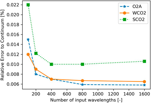
FIGURE 5. Modeling error in percent relative to continuum for different number of input wavelengths. O2A-band is shown with blue stars, WCO2-band with orange dots, and SCO2-band with green squares.

For the O2A-band, the error does not decrease for adding more than 800 input wavelengths. The increase in accuracy for the WCO2-band and SCO2-band saturates even earlier at 400 wavelengths.

The graph illustrates how the proposed approach can be tuned to either prioritize computation cost over error (small number of input wavelengths) or accuracy over computational cost (large number of input wavelengths).

The errors are even smaller when we compare the spectra after convolving them to the 1,016 instrument channels of OCO-2. This further reduces the error of the O2A-band with 800 input wavelengths from 0.0048% to 0.0035%. For the WCO2-band and SCO2-band with 400 input wavelengths, the error is reduced from 0.0064% to 0.0042% and 0.01% to 0.0059%, respectively.

4.2.2 Error Dependence on State Space

We analyzed the model error with respect to various state variables. For most variables, there is no clear dependence. However, a clear dependence of the modeling error is found with respect to the path length of the solar radiation through the atmosphere, with the error increasing for longer path lengths. This effect is similar in magnitude for all three instrument channels (see Figure 6) and indicates that our assumption, $\widehat{\mathit{i}}$ can be expressed as $\mathrm{e}\mathrm{x}\mathrm{p}(\text{ln}\left(\mathit{i}\right) \mathit{A})$ (see Eq. 2), is increasingly violated for these viewing geometries and solar zenith angles. This could be due to scattering by aerosols, light refraction by the atmospheric density gradient, or other effects not captured in Eq. 2. Additionally, we find some dependencies of modeling errors associated with the effects of thin clouds that were not flagged by the O2A-band preprocessor (ABP). One quantity associated with clouds in a fairly quantitative way is dp_abp which represents the retrieved surface pressure minus the surface pressure from a meteorological forecast model. For dp_abp, we notice increasing modeling errors when it deviates more than 1,000 Pa from zero, indicating that clouds challenge the proposed speed-up approach.

FIGURE 6

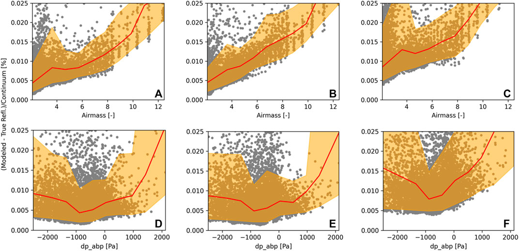
FIGURE 6. Reconstruction error in percent relative to continuum with respect to airmass for the (A) O2A-band, (B) WCO2-band, (C) SCO2-band as well as dp_abp for the (D) O2A-band, (E) WCO2-band, and (F) SCO2-band. The mean is shown in red, the 5th and 95th percentile in orange, and the error of individual spectra with grey dots.

4.2.3 Sensitivity to Clouds

As discussed previously, soundings with strong cloud contamination (as identified by the ABP cloud flag) are excluded from OCO-2/3 processing and were therefore omitted in the training and testing sets in this study. However, this restricts the use of our developed methodology to cloud free RTM calculations. To probe whether our approach is generalizable to cloudy scenes, which might be important for other applications (e.g., extracting cloud or aerosol properties from OCO-2/3 observations (Richardson and Stephens, 2018; Richardson et al., 2019; Zeng et al., 2020)), we fit a separate correlation matrix to spectra that contain both, cloud-free and cloud contaminated spectra following the same procedure described in Section 3.1. The results are shown in Table 2. For cloud-free soundings, the error of the model trained with cloud contaminated and cloud-free spectra “mixed” has a similar performance to our model trained on cloud-free data only. However, applying the “mixed” model on cloud contaminated spectra increases the average modeling error by roughly 50% for all three bands, which itself is possibly still low enough for retrieving cloud or aerosol properties. For comparison, the last row shows the performance for the models trained and tested on cloud-free spectra, as proposed in this study to be used in the ACOS X_CO2 retrieval.

TABLE 2

TABLE 2. Modeling error in percent relative to continuum for models trained with spectra including cloud contamination (mixed) and tested on cloud-free and cloud contaminated spectra. The last row shows the performance for the models fit with cloud-free data for comparison (as proposed).

4.2.3 Land vs. Ocean

The developed approach uses the same correlation matrix, for glint observations over the ocean and nadir observations over land. Table 3 shows what performance gains would be enabled if two separate matrices would be used for each observation type. While this would make the implementation of the RTM speed-up slightly more complicated, it would reduce the error another 0.001%–0.004% depending on the instrument channel. The biggest improvement would be for land nadir observations in the SCO2-band. Since we aim to keep our developed approach as simple and general as possible, we propose to use only one model per channel without differentiating by observation type.

TABLE 3

TABLE 3. Modeling error in percent relative to continuum for models trained with land nadir and ocean glint soundings. The last two rows show the performance for the models fit with a mix of land and ocean (as proposed).

4.2.4 Wavelength-Dependent Error

So far, we have discussed only the average error for each band. It is important to further understand how this error is distributed across the various wavelengths. An example of a representative modeled spectrum of each band and its error before and after convolving it with the OCO-2/3 instrument line function is shown in Figure 7. The three spectra were selected from the testing set and contain an RMSE close to the average RMSE of each band. For all three bands, the difference in modeled and original radiance is almost invisible when overplotting both spectra. Looking at the difference plot of the O2A-band, the biggest errors are in the continuum. Furthermore, after convolution, we see some discrepancy around 762 nm on the order of 0.01%. For the modeled WCO2-band, the error is more evenly distributed with some overestimation by the model around 1,598 nm. The error in the modeled SCO2-band seems equally distributed as well.

FIGURE 7

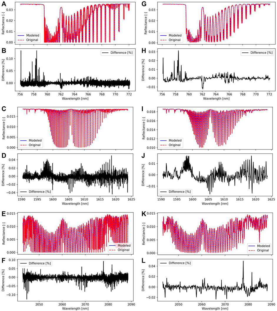
FIGURE 7. Modeled spectra and associated errors for one representative sounding, before and after convolution with the OCO-2 instrument lineshape function, for each instrument channel. O2A-band (A,B) after convolution (G,H); WCO2-band (C,D) after convolution (I,J); SCO2-band (E,F) after convolution (K,L). The modeled spectra are shown in blue, the original spectra in red, and the difference in percent relative to the continuum in black.

Analyzing the wavelength-dependent error over the complete testing set, we find no systematic biases in any of the wavelengths for all three channels (see Figure 8) with the absolute average error being below 0.1% at all wavelengths of each band. The 5th to 95th percentile is mostly symmetrically centered around zero. For the O2A and WCO2 bands, 90% of the modeled spectra have an error of less than ±0.02% on a per-wavelength basis. For the SCO2 band, the error is approximately twice that of the O2A band.

FIGURE 8

FIGURE 8. Modeling error over the full testing set for each wavelength of the O2A-band (A), WCO2-band (B), and SCO2-band (C). The mean error is shown in black, the 5th to 95th percentile is shown in turquoise.

5 Discussion

5.1 Dependency of Reconstructed Spectra to Model Inputs

To build intuition of how individual wavelengths contribute to the modeled spectrum, we further contrast the relative importance of the 100 most important wavelengths. The radiance at each of the 100 wavelengths is perturbed independently by 1%, the full spectrum is reconstructed from the perturbed spectrum, and the RMSE in percent relative to continuum is evaluated. This is repeated for each of the 100 input wavelengths and each spectrum in the testing set. The average increase in error to this perturbation is shown in Figure 9 for the O2A-band, WCO2-band, and SCO2-band as a function of mean reflectance. All three bands show a similar dependence in their sensitivity to mean reflectance. Wavelengths at which most of the incoming sunlight is attenuated have a smaller sensitivity compared to wavelength where most radiation is scattered.

FIGURE 9

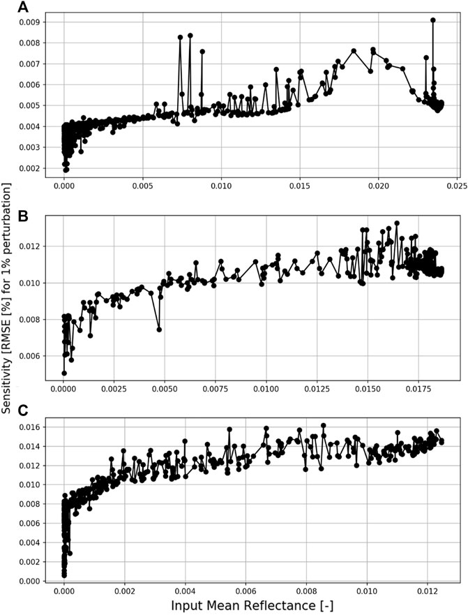
FIGURE 9. Sensitivity of model error to individual input wavelengths for O2A-band (A), WCO2-band (B), and SCO2-band (C). Note: the y- and x-axis have different scales for each plot.

5.2 Comparison to Linear Interpolation

The current method to reduce the number of RTM evaluations relies on linear interpolation between radiances at neighboring wavelengths. While this method allows reducing the number of necessary RTM calculations, it requires an order of magnitude of more wavelengths than the method proposed in this manuscript (see Figure 10). This is due to the inability of the current method to exploit the correlations of non-neighboring wavelengths, for example, absorption features of the same gas. However, due to the simplicity of the linear interpolation, it generalizes well to new data and is relatively robust to small spectroscopic updates to the RTM. In contrast, the method proposed here will require retraining the model if virtually any updates to the RTM are made, for example, updated absorption profiles for trace gases.

FIGURE 10

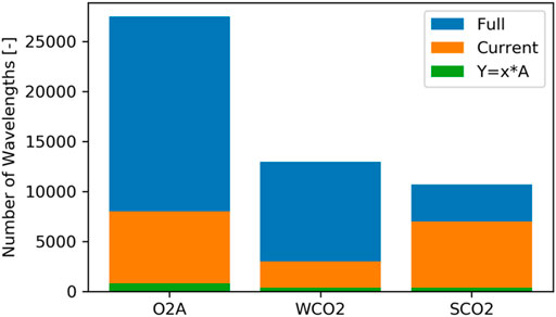
FIGURE 10. Number of required monochromatic RTM calculations to model a complete spectrum: calculating radiances at each wavelength (“Full”: blue), the current approach using linear interpolation of neighboring wavelengths (“Current”: orange), and the approach proposed in this manuscript (“Y = x*A”: green). The number of required RTM calculations is approximately proportional to the computational cost. Comparisons are shown for each OCO-2 instrument band.

As mentioned earlier, the use case for our proposed method only addresses the computational cost associated with the low-accuracy calculations of the RTM used by OCO-2, which make up approximately 57% of the processing time for a given retrieval. To evaluate the speed-up for our application, we calculated 100 spectra with the RTM, including low-accuracy, high-accuracy calculations, and convolution to the OCO-2 instrument channels. The presented approach takes on average 7.1 s for one sounding and the associated spectra for all three instrument channels on a single CPU. In comparison, the current approach takes 13.1 s and calculating all wavelengths directly takes 16.7 s. This illustrates how we effectively reduced the most expensive part of the RTM to being negligible and further acceleration needs to come from other parts of the RTM, for example, the high-accuracy calculations.

5.3 How Much Training Data Are Needed?

The presented approach can speed up a forward model by orders of magnitude. However, it first requires building a training set with repeated evaluations of a RTM. The additional computational cost of building this initial training set needs to be considered together with the reduction in computational cost provided by the proposed method. The cost of building the training set directly depends on how many spectra are needed to fit the correlation matrix. After a certain point, the correlation matrix cannot be further constrained even if more training data would be available. To test how many spectra are required, we sampled every nth spectrum from the training set, with n = 1, 2, 4, 25 and fit the correlation matrix with those reduced training sets. The error evaluation was carried out on the same test set for all models. The number of training iterations was held constant across all models to compensate for the changing training set sizes. Figure 11 shows the error for the three instrument channels and how they depend on the size of the training set. For the O2A-band and SCO2-band, there are negligible improvements for more than 6,000 spectra. The model for the WCO2-band does not show a strong dependency on training set size and can be successfully trained with only 1,000 spectra (given that they adequately capture the variability of the full state space). Thus, compared to the roughly 100,000 cloud-free spectra OCO-2 obtains every day, the computational cost of making the initial training set is negligible. The small training set size is a direct result of the simplicity of our model, limited to a single matrix that needs to be determined.

FIGURE 11

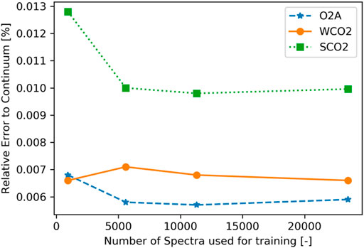
FIGURE 11. Modeling error in percent relative to continuum for different training set sizes. O2A-band is shown with blue stars, WCO2-band with orange dots, and SCO2-band with green squares.

6 Conclusion

The presented research addressed only the acceleration of one element of the OE retrieval, namely, the low-accuracy RTM calculations. These calculations consume about half of the total time needed for each OE iteration. Thus, even with the demonstrated speed up of more than an order of magnitude, we will be able to accelerate the OCO-2/3 retrieval only by a factor of two. Reducing the computation needed for the high-accuracy RTM, calculations that take up most of the remaining computing time should be addressed going forward. The purpose of these high-accuracy RTM calculations is to correct the low-accuracy calculations to account for computationally expensive multiple scattering. Compared to fully modeling the low-accuracy calculations, the dimensionality of these correction terms is much smaller. Thus, deriving the correction factors directly from the state vector using machine learning might be a viable option and would allow to speed up the whole OE retrieval by an order of magnitude compared to the current implementation.

We showed that high-resolution spectra in the O2A-band, WCO2-band, and SCO2-band that contain tens of thousands of wavelengths can be modeled from a small subset of wavelengths (hundreds) to better than 0.01%. The presented approach is tunable to a desired speed-accuracy trade-off. The described technique allows to significantly speed up a RTM for the discussed wavelength bands by an order of magnitude. This is especially important for OE retrievals that heavily rely on RTM evaluations in each retrieval iteration as applied to the retrieval of X_CO2 from OCO-2/3 observations. The presented modeling approach results in spectra that are free of systematic biases and will be used operationally for OCO-2/3 retrievals. Our approach is simple, robust, requires little training data and can be readily expanded to wavelength ranges beyond the three discussed bands.

Data Availability Statement

The original contributions presented in the study are included in the article/Supplementary Material; further inquiries can be directed to the corresponding author.

Author Contributions

SM led the research and wrote the first draft of the manuscript. GM provided the data. GM, CO’D, and VN provided guidance. All authors contributed to manuscript revision and read and approved the submitted version.

Funding

This research was carried out at the Jet Propulsion Laboratory, California Institute of Technology, under a contract with the National Aeronautics and Space Administration (80NM0018D0004).

Conflict of Interest

The authors declare that the research was conducted in the absence of any commercial or financial relationships that could be construed as a potential conflict of interest.

Publisher’s Note

All claims expressed in this article are solely those of the authors and do not necessarily represent those of their affiliated organizations, or those of the publisher, the editors, and the reviewers. Any product that may be evaluated in this article, or claim that may be made by its manufacturer, is not guaranteed or endorsed by the publisher.

References

Abadi, M., Barham, P., Chen, J., Chen, Z., Davis, A., Dean, J., et al. (2016). Tensorflow: A System for Large-Scale Machine Learning.” in Paper presented at the 12th USENIX symposium on operating systems design and implementation (OSDI 16), Savannah, GA, November 2-4, 2016.

Google Scholar

Bai, W., Zhang, P., Zhang, W., Ma, G., Qi, C., and Liu, H. (2020). A Fast and Accurate Vector Radiative Transfer Model for Simulating the Near-Infrared Hyperspectral Scattering Processes in Clear Atmospheric Conditions. J. Quantitative Spectrosc. Radiat. Transf. 242, 106736. doi:10.1016/j.jqsrt.2019.106736

CrossRef Full Text | Google Scholar

Bösch, H., Toon, G. C., Sen, B., Washenfelder, R. A., Wennberg, P. O., Buchwitz, M., et al. (2006). Space-based Near-Infrared CO₂ Measurements: Testing the Orbiting Carbon Observatory Retrieval Algorithm and Validation Concept Using SCIAMACHY Observations over Park Falls, Wisconsin. J. Geophys. Res. 111 (D23), 7080. doi:10.1029/2006JD007080

CrossRef Full Text | Google Scholar

Brence, J., Tanevski, J., Adams, J., Malina, E., and Džeroski, S. (2022). Surrogate Models of Radiative Transfer Codes for Atmospheric Trace Gas Retrievals from Satellite Observations. Mach. Learn, 1–27. doi:10.1007/s10994-022-06155-2

CrossRef Full Text | Google Scholar

Brodrick, P. G., Thompson, D. R., Fahlen, J. E., Eastwood, M. L., Sarture, C. M., Lundeen, S. R., et al. (2021). Generalized Radiative Transfer Emulation for Imaging Spectroscopy Reflectance Retrievals. Remote Sens. Environ. 261, 112476. doi:10.1016/j.rse.2021.112476

CrossRef Full Text | Google Scholar

Bue, B. D., Thompson, D. R., Deshpande, S., Eastwood, M., Green, R. O., Natraj, V., et al. (2019). Neural Network Radiative Transfer for Imaging Spectroscopy. Atmos. Meas. Tech. 12 (4), 2567–2578. doi:10.5194/amt-12-2567-2019

CrossRef Full Text | Google Scholar

Clough, S. A., Shephard, M. W., Mlawer, E. J., Delamere, J. S., Iacono, M. J., Cady-Pereira, K., et al. (2005). Atmospheric Radiative Transfer Modeling: A Summary of the AER Codes. J. Quantitative Spectrosc. Radiat. Transf. 91 (2), 233–244. doi:10.1016/j.jqsrt.2004.05.058

CrossRef Full Text | Google Scholar

Connor, B. J., Boesch, H., Toon, G., Sen, B., Miller, C., and Crisp, D. (2008). Orbiting Carbon Observatory: Inverse Method and Prospective Error Analysis. J. Geophys. Res. 113 (D5), a–n. doi:10.1029/2006JD008336

CrossRef Full Text | Google Scholar

Duan, M., Min, Q., and Li, J. (2005). A Fast Radiative Transfer Model for Simulating High-Resolution Absorption Bands. J. Geophys. Res. 110 (D15). 5590. doi:10.1029/2004JD005590

CrossRef Full Text | Google Scholar

Efremenko, D., Doicu, A., Loyola, D., and Trautmann, T. (2014). Optical Property Dimensionality Reduction Techniques for Accelerated Radiative Transfer Performance: Application to Remote Sensing Total Ozone Retrievals. J. Quantitative Spectrosc. Radiat. Transf. 133, 128–135. doi:10.1016/j.jqsrt.2013.07.023

CrossRef Full Text | Google Scholar

Eldering, A., O'Dell, C. W., Wennberg, P. O., Crisp, D., Gunson, M. R., Viatte, C., et al. (2017). The Orbiting Carbon Observatory-2: First 18 Months of Science Data Products. Atmos. Meas. Tech. 10 (2), 549–563. doi:10.5194/amt-10-549-2017

CrossRef Full Text | Google Scholar

Eldering, A., Taylor, T. E., O'Dell, C. W., and Pavlick, R. (2019). The OCO₃ Mission: Measurement Objectives and Expected Performance Based on 1 Year of Simulated Data. Atmos. Meas. Tech. 12 (4), 2341–2370. doi:10.5194/amt-12-2341-2019

CrossRef Full Text | Google Scholar

Gao, M., Franz, B. A., Knobelspiesse, K., Zhai, P.-W., Martins, V., Burton, S., et al. (2021). Efficient Multi-Angle Polarimetric Inversion of Aerosols and Ocean Color Powered by a Deep Neural Network Forward Model. Atmos. Meas. Tech. 14 (6), 4083–4110. doi:10.5194/amt-14-4083-2021

CrossRef Full Text | Google Scholar

Gómez-Dans, J. L., Lewis, P. E., and Disney, M. (2016). Efficient Emulation of Radiative Transfer Codes Using Gaussian Processes and Application to Land Surface Parameter Inferences. Remote Sens. 8 (2), 119. Retrieved from https://www.mdpi.com/2072-4292/8/2/119. doi:10.3390/rs8020119

CrossRef Full Text | Google Scholar

Goody, R., West, R., Chen, L., and Crisp, D. (1989). The Correlated-K Method for Radiation Calculations in Nonhomogeneous Atmospheres. J. Quantitative Spectrosc. Radiat. Transf. 42 (6), 539–550. doi:10.1016/0022-4073(89)90044-7

CrossRef Full Text | Google Scholar

Han, K., Wang, Y., Zhang, C., Li, C., and Xu, C. (2018). Autoencoder Inspired Unsupervised Feature Selection.” in Paper presented at the 2018 IEEE International Conference on Acoustics, Speech and Signal Processing (ICASSP), Calgary, Alberta, April 15-20, 2018. doi:10.1109/icassp.2018.8462261

CrossRef Full Text | Google Scholar

Hasekamp, O. P., and Butz, A. (2008). Efficient Calculation of Intensity and Polarization Spectra in Vertically Inhomogeneous Scattering and Absorbing Atmospheres. J. Geophys. Res. 113 (D20). 10379. doi:10.1029/2008JD010379

CrossRef Full Text | Google Scholar

Kingma, D. P., and Ba, J. (2014). Adam: A Method for Stochastic Optimization. arXiv. doi:10.48550/arxiv.1412.6980

CrossRef Full Text | Google Scholar

Kuhlmann, G., Broquet, G., Marshall, J., Clément, V., Löscher, A., Meijer, Y., et al. (2019). Detectability of CO₂; Emission Plumes of Cities and Power Plants with the Copernicus Anthropogenic CO₂ Monitoring (CO₂M) Mission. Atmos. Meas. Tech. 12 (12), 6695–6719. doi:10.5194/amt-12-6695-2019

CrossRef Full Text | Google Scholar

Lacis, A. A., and Oinas, V. (1991). A Description of the Correlatedkdistribution Method for Modeling Nongray Gaseous Absorption, Thermal Emission, and Multiple Scattering in Vertically Inhomogeneous Atmospheres. J. Geophys. Res. 96 (D5), 9027–9063. doi:10.1029/90JD01945

CrossRef Full Text | Google Scholar

Le, T., Liu, C., Yao, B., Natraj, V., and Yung, Y. L. (2020). Application of Machine Learning to Hyperspectral Radiative Transfer Simulations. J. Quantitative Spectrosc. Radiat. Transf. 246, 106928. doi:10.1016/j.jqsrt.2020.106928

CrossRef Full Text | Google Scholar

Liu, X., Smith, W. L., Zhou, D. K., and Larar, A. (2006). Principal Component-Based Radiative Transfer Model for Hyperspectral Sensors: Theoretical Concept. Appl. Opt. 45 (1), 201–209. doi:10.1364/AO.45.000201

PubMed Abstract | CrossRef Full Text | Google Scholar

Moncet, J.-L., Uymin, G., Liang, P., and Lipton, A. E. (2015). Fast and Accurate Radiative Transfer in the Thermal Regime by Simultaneous Optimal Spectral Sampling over All Channels. J. Atmos. Sci. 72 (7), 2622–2641. doi:10.1175/jas-d-14-0190.1

CrossRef Full Text | Google Scholar

Moore III, B., Crowell, S. M. R., Rayner, P. J., Kumer, J., O'Dell, C. W., O'Brien, D., et al. (2018). The Potential of the Geostationary Carbon Cycle Observatory (GeoCarb) to Provide Multi-Scale Constraints on the Carbon Cycle in the Americas. Front. Environ. Sci. 6, 109. doi:10.3389/fenvs.2018.00109

CrossRef Full Text | Google Scholar

Natraj, V., Jiang, X., Shia, R.-l., Huang, X., Margolis, J. S., and Yung, Y. L. (2005). Application of Principal Component Analysis to High Spectral Resolution Radiative Transfer: A Case Study of the Band. J. Quantitative Spectrosc. Radiat. Transf. 95 (4), 539–556. doi:10.1016/j.jqsrt.2004.12.024

CrossRef Full Text | Google Scholar

O'Dell, C. W. (2010). Acceleration of Multiple-Scattering, Hyperspectral Radiative Transfer Calculations via Low-Streams Interpolation. J. Geophys. Res. 115 (D10), 12803. doi:10.1029/2009JD012803

CrossRef Full Text | Google Scholar

O'Dell, C. W., Connor, B., Bösch, H., O'Brien, D., Frankenberg, C., Castano, R., et al. (2012). The ACOS CO₂ Retrieval Algorithm - Part 1: Description and Validation against Synthetic Observations. Atmos. Meas. Tech. 5 (1), 99–121. doi:10.5194/amt-5-99-2012

CrossRef Full Text | Google Scholar

O'Dell, C. W., Eldering, A., Wennberg, P. O., Crisp, D., Gunson, M. R., Fisher, B., et al. (2018). Improved Retrievals of Carbon Dioxide from Orbiting Carbon Observatory-2 with the Version 8 ACOS Algorithm. Atmos. Meas. Tech. 11 (12), 6539–6576. doi:10.5194/amt-11-6539-2018

CrossRef Full Text | Google Scholar

Pal, A., Mahajan, S., and Norman, M. R. (2019). Using Deep Neural Networks as Cost‐Effective Surrogate Models for Super‐Parameterized E3SM Radiative Transfer. Geophys. Res. Lett. 46 (11), 6069–6079. doi:10.1029/2018GL081646

CrossRef Full Text | Google Scholar

Reichstein, M., Camps-Valls, G., Stevens, B., Jung, M., Denzler, J., Carvalhais, N., et al. (2019). Deep Learning and Process Understanding for Data-Driven Earth System Science. Nature 566 (7743), 195–204. doi:10.1038/s41586-019-0912-1

PubMed Abstract | CrossRef Full Text | Google Scholar

Richardson, M., Leinonen, J., Cronk, H. Q., McDuffie, J., Lebsock, M. D., and Stephens, G. L. (2019). Marine Liquid Cloud Geometric Thickness Retrieved from OCO₂'s Oxygen A-Band Spectrometer. Atmos. Meas. Tech. 12 (3), 1717–1737. doi:10.5194/amt-12-1717-2019

CrossRef Full Text | Google Scholar

Richardson, M., and Stephens, G. L. (2018). Information Content of OCO₂ Oxygen A-Band Channels for Retrieving Marine Liquid Cloud Properties. Atmos. Meas. Tech. 11 (3), 1515–1528. doi:10.5194/amt-11-1515-2018

CrossRef Full Text | Google Scholar

Sioris, C. E., and Evans, W. F. J. (2000). Impact of Rotational Raman Scattering in the O₂Aband. Geophys. Res. Lett. 27 (24), 4085–4088. doi:10.1029/2000GL012231

CrossRef Full Text | Google Scholar

Stegmann, P. G., Johnson, B., Moradi, I., Karpowicz, B., and McCarty, W. (2022). A Deep Learning Approach to Fast Radiative Transfer. J. Quantitative Spectrosc. Radiat. Transf. 280, 108088. doi:10.1016/j.jqsrt.2022.108088

CrossRef Full Text | Google Scholar

Sun, Y., Frankenberg, C., Wood, J. D., Schimel, D. S., Jung, M., Guanter, L., et al. (2017). OCO₂ Advances Photosynthesis Observation from Space via Solar-Induced Chlorophyll Fluorescence. Science 358 (6360), eaam5747. doi:10.1126/science.aam5747

PubMed Abstract | CrossRef Full Text | Google Scholar

Svendsen, D. H., Martino, L., and Camps-Valls, G. (2020). Active Emulation of Computer Codes with Gaussian Processes - Application to Remote Sensing. Pattern Recognit. 100, 107103. doi:10.1016/j.patcog.2019.107103

CrossRef Full Text | Google Scholar

Swinehart, D. F. (1962). The Beer-Lambert Law. J. Chem. Educ. 39 (7), 333. doi:10.1021/ed039p333

CrossRef Full Text | Google Scholar

Vicent, J., Verrelst, J., Rivera-Caicedo, J. P., Sabater, N., Munoz-Mari, J., Camps-Valls, G., et al. (2018). Emulation as an Accurate Alternative to Interpolation in Sampling Radiative Transfer Codes. IEEE J. Sel. Top. Appl. Earth Obs. Remote Sens. 11 (12), 4918–4931. doi:10.1109/JSTARS.2018.2875330

CrossRef Full Text | Google Scholar

Wiscombe, W. J., and Evans, J. W. (1977). Exponential-sum Fitting of Radiative Transmission Functions. J. Comput. Phys. 24 (4), 416–444. doi:10.1016/0021-9991(77)90031-6

CrossRef Full Text | Google Scholar

Zeng, Z.-C., Chen, S., Natraj, V., Le, T., Xu, F., Merrelli, A., et al. (2020). Constraining the Vertical Distribution of Coastal Dust Aerosol Using OCO₂ O₂ A-Band Measurements. Remote Sens. Environ. 236, 111494. doi:10.1016/j.rse.2019.111494

CrossRef Full Text | Google Scholar