Latitudes and land use: Global biome shifts in vegetation persistence across three decades

Introduction

The dynamics of terrestrial vegetation are shifting globally due to environmental changes, with potential repercussions for the proper functioning of the Earth system and provision of ecosystem services. These changes are most apparent in the vegetation composition and/or structure, with shifts in species dominance and/or abundance, and changes in phenology. In some cases, there may be a complete loss of vegetation cover. Such changes can alter the local climate, hydrology, and soil properties, affecting a range of other ecosystem processes. The consequences of these vegetation changes can be far-reaching, impacting human societies through alterations in the provision of food, water, fuel, and timber resources, as well as affecting carbon storage and greenhouse gas emissions. Therefore, it is essential to monitor and quantify landscape level vegetation change to anticipate and adapt to the consequences of environmental change (Winkler et al., 2021; Potapov et al., 2022).

The vegetation of the Earth is constantly changing in response to a variety of biotic and abiotic factors. The study of vegetation change, and the methods used to monitor it, have in themselves been found to significantly impact the findings. Vegetation variability is a function of many factors, including climate, land use, and disturbance regime. Climate variability, for example, can cause changes in vegetation type, composition, and distribution. Land use can also impact vegetation, through activities such as deforestation, agriculture, and urbanization (Winkler et al., 2021; Friedl et al., 2022; Potapov et al., 2022). Disturbance regimes (such as fire or grazing) can also affect vegetation changes. Monitoring vegetation change is essential to understanding the health of our ecosystems. Vegetation provides critical ecosystem services such as carbon sequestration, water and soil conservation, and habitat for wildlife. Changes in vegetation can therefore have profound impacts on the environment and human wellbeing (Winkler et al., 2021).

There is large variability in the way vegetation responds to changes in the environment. This variability is due to a range of factors, including the species composition of vegetation, the growth form of plants (e.g., trees vs. shrubs), the level of disturbance, climatic conditions, and the soil type. For example, forests are more likely to respond slowly to environmental change than grasslands or savannas, due to the longer life span of trees. In addition, deciduous species are generally more responsive than evergreen species, as annual leaf drop means a quicker response to short-term changes in conditions. The magnitude and direction of vegetation change also varies regionally. In general, vegetation changes are more pronounced in the northern hemisphere than in the southern hemisphere, due to the greater land area and more diverse range of vegetation types. Finally, vegetation changes are typically more rapid in the tropics than in other regions, due to the higher levels of radiation and precipitation.

The study of vegetation change is essential to understanding the health of our ecosystems and the potential impacts of environmental change on human wellbeing. A variety of monitoring techniques are available to researchers, each with its own advantages and disadvantages. The selection of the most appropriate method(s) depends on the vegetation type of interest, the scale of analysis, and the desired level of detail. There are a variety of methods used to monitor vegetation change. Remote sensing techniques, such as satellite imagery, are commonly used to detect changes in vegetation cover. Ground-based monitoring, such as vegetation surveys, can provide detailed information on vegetation type and composition. Finally, model-based approaches can be used to simulate vegetation change under different scenarios. It is important to monitor vegetation change in order to anticipate and adapt to the consequences of environmental change.

Remote sensing is a powerful tool for monitoring vegetation change, as it allows for repeated measurements over large areas. Satellite-based remote sensing provides global coverage and can be used to track changes in vegetation cover and structure. By measuring the reflectance of vegetation in different spectral bands, we can produce an index known as the Normalized Difference Vegetation Index (NDVI). This index can be used to track changes in vegetation health and density over time. The Advanced Very High Resolution Radiometer (AVHRR) is a satellite sensor that is often used for this purpose. AVHRR data has been used to monitor trends in global vegetation cover since the early 1980s (de Jong et al., 2012; Cortes et al., 2021). More recently, satellite based NDVI products have become available from other sensors, such as the Moderate Resolution Imaging Spectroradiometer (MODIS). These products provide higher spatial resolution and more frequent coverage, making them ideal for tracking short-term changes in vegetation cover. Vegetation monitoring is important for a variety of reasons. Changes in vegetation cover can be used to track the progress of land degradation and deforestation. Additionally, NDVI data can be used to monitor the effects of drought and other environmental stresses on vegetation health. Ultimately, satellite remote sensing provides a cost-effective means of monitoring large areas of vegetation over time, which is essential for understanding and managing the world’s natural resources (Southworth and Muir, 2021).

Vegetation is viewed as one of the more significant elements in the land-atmosphere system (Liu et al., 2020), involved in maintaining the water cycle, GPP (Gross Primary Productivity), and the fluxes of carbon between the atmosphere and land (Yao et al., 2019). In addition, vegetative biomass (above-ground) is also one of the chief sources of carbon sink, hence modulating ecosystem services via carbon sequestration (Tian et al., 2021). With the increase in the concentration of carbon dioxide (CO₂) in the atmosphere owing to anthropogenic stresses, the global vegetation cover and amount, often referred to as “greenness,” is also increasing, and this greening is most often attributed to CO₂ fertilization (it speeds up photosynthesis and limits leaf transpiration of plants) and afforestation (Lenka and Lal, 2012). Studies have suggested an increase in greenness is expected to continue until 2,100, which will alter the dynamics of vegetation globally (Zhu et al., 2016; Liu et al., 2022). Thus, monitoring such change is indispensable given their susceptibility to anthropogenic pressures (land-use change and release of CO₂), including those associated with climatic variability (atmospheric temperature, humidity, and precipitation) and the importance of monitoring change and understanding the drivers is of critical importance (de Jong et al., 2012; 2013).

Global greening is a phenomenon that has been studied over the last few decades, and most evidence details such global greening signals from the beginning of the satellite record in the early 1980s (Nemani and Running 1997; Nemani et al., 2003; de Jong et al., 2012; 2013; Zhu et al., 2016; Piao et al., 2020; Jiang et al., 2022). It was only the development of satellite technologies that led us to be able to monitor such changes globally and then link these greening signals to potential drivers of change. Globally, the dominant driver of greening which has been identified relates to CO₂ fertilization (Zhu et al., 2016; Piao et al., 2020) with additional drivers becoming important only at more regional scales. Most global greening studies have focused on satellite data as the variable under study, and most often have utilized vegetation metrics, such as NDVI, a measure which links to the amount and health of green vegetation biomass, often used as a proxy for net primary production (NPP) globally (Piao et al., 2020). Such greenness measures are thus used to identify trends of NDVI as measured over space and time, which may relate to vegetation type; fertilization of plant growth (in the form of more leaves, bigger leaves or even different species); the start, length and duration of the growing season; and thus the signal of greening measured, and also potential changes in crop production and multiple crop cycles. As such, the observed signal is an index representing a wide range of possible ground level changes, and while some studies do integrate limited ground-based data, given that many such studies are globally focused, real ground truthing is not always feasible. Modelling is frequently utilized to link the greening measures to possible drivers of change. Such modelling exercises clearly highlight the role of increased CO₂ concentration as the main driver of the observed greening, with matches over seasons and years.

Regional scale drivers have been identified as land cover change and changing management, such as reforestation, afforestation and improved agricultural practices (irrigation, improved crop types, intensification, etc.), nitrogen deposition and changing climate (especially changes in temperature and precipitation patterns and ranges) (Nemani and Running 1997; Xiao and Moody 2005; Zhu et al., 2016; Piao et al., 2020). Climatic drivers have also been identified, with different regions globally responding to different drivers. More climate focused drivers were identified by Xiao and Moody (2005), whereas Chen et al. (2019) focused on human land-use management, specifically related to agricultural lands and system improvements in China and India as the leading cause of greening. Across many drylands regions precipitation change is linked most directly to the greening signal (Herrmann et al., 2005) and concomitantly, linked to decreases in NPP related to large-scale droughts and a drying trend seen in the Southern Hemisphere (Zhao and Running, 2010).

One limitation of most of these studies of greening, as highlighted by de Jong et al. (2012) is related to the type of data used within such studies. Specifically, all of the greening studies have utilized remotely sensed time-series of vegetation indices, most of which have seasonality and serial auto-correlation, and while the studies attempted to correct for these trends using such techniques as harmonic regression, linear models with non-parametric components for seasonality, time series development from calendar days, and similar techniques, de Jong et al. (2012) found the results in terms of greening or browning, varied significantly, depending on the methods used. In addition, no single ideal method was identified and the difficulty of comparisons across different methods and outcomes was highlighted. In response to such difficulties, as identified by multiple researchers, the creation of a simple, statistically valid, and repeatable method has become increasingly warranted. NDVI time series can be used to study global vegetation change in several ways. For example, NDVI data can be used to map the areal extent of vegetation changes, as well as to quantify the magnitude and direction of those changes. NDVI data can also be used to assess the temporal patterns of vegetation change, allowing scientists to identify possible drivers of those changes. Finally, NDVI data can be used to estimate net primary productivity, which is an important measure of ecosystem health. NDVI time series also provides a way to assess the statistical significance of changes in vegetation greenness at a pixel level (Southworth and Muir, 2021). This is important for understanding whether the observed changes are due to natural variability or to anthropogenic activity.

Waylen et al. (2014) developed an NDVI-derived time-series of remotely sensed data products within which the user could define the appropriate statistical significance for their given research question. The directional persistence (D) metric allowed for the analysis of change in NDVI relative to a fixed benchmark value—which could be defined as a period, e.g., the beginning of a time series such as in analysis of greening, or an event, e.g., a drought, thereby facilitating a much more detailed and nuanced understanding of a given landscape. The D statistic borrows heavily from the theory associated with random walk processes (Wilson and Kirkby, 1980), in which each positive departure from the previous value in the time series cumulates the statistic by +1, and each negative departure by −1. The null hypothesis against which the statistic can be tested is that the statistics for a time series is not significantly different from zero. Critical values of the test statistic at various significance levels and for varying length of time series are derived from Monte Carlo simulations. The statistic has the benefits of being easy to calculate, readily interpreted in terms of the natural processes, comparable spatially, and the capability of being tested for significance by a method based in statistical theory. This metric has been tested at a smaller scale to understand vegetation persistence across Florida (Tsai et al., 2014) and within specific ecosystems types more broadly (Southworth et al., 2016; Bunting et al., 2018). Results have been very promising in terms of their innovation and in making the continuous vegetation metrics approach both more useful and more rigorous for use in global change studies.

Utilizing the length of the satellite data record and such measures as the D metric, such systematic quantification of vegetation change globally can be derived, and then interpreted with a view to better understand the spatial patterns and trends and how these relate to different global biomes and their land use diversity. Given the recent focus on greening papers to attempt to better determine the more regional-scale drivers of change, often completed at a more regional focus, e.g., China, India (Chen et al., 2019) or review papers which highlight the need for this regional level view at this time (Piao et al., 2020), our research will utilize this new metric, D, to evaluate global trends in vegetation persistence since the more reliable records of remotely sensed data began in the early 1980s. Specifically though, we will focus on the differences in patterns of vegetation persistence as a function of their biomes, and also the actual land use diversity at the pixel level, as determined by FAO data (FAO 2010 data available at FAO.org). Biomes are selected as the broad unit of analysis, as these represent similar ecosystems which, by definition, share comparable processes and major vegetation types wherever they are found. Studying at the level of biomes is important because they may display substantial variation in the extent of change, face different drivers of change, and there may be differences in the options for mitigating or managing these drivers. Biomes are important, but so is land cover and related land use diversity. As such, even within our biomes, we will also account for the land use diversity, as stated by FAO in their 2010 global product (FAO.org), which will reflect the final use or end point of the time series in terms of land use with a reputable data source such as FAO which is readily available and downloadable for analysis. In addition, FAO products are considered comparable globally. As such, this research will cover over 30 years of vegetation persistence analysis at the biomes level, accounting for land use diversity and evaluating at a seasonal scale. Seasons are something that show different patterns and as such, it is important to both explain and account for these possible phenological signals.

This research addresses the following questions: 1) Globally, does the pattern of Vegetation Persistence, or D, match the findings demonstrated in previous global greening papers, and do the observable patterns and trends match up spatially? 2) Do these trends, most of which were analyzed at an annual time step, hold constant across seasons or do trends vary within the growing season? 3) How do the trends and patterns vary across the different biomes and are there obvious winners or losers to the greening trend? Lastly, 4) how does land use diversity impact these biomes-based trends and findings? Given the focus on the metric D as opposed to continuous indices measures of NDVI, this research bypasses many of the concerns of methods utilized potentially influencing the trend of the findings (de Jong et al., 2012), while also providing a very simple and easily understandable and replicable final product.

Materials and methods

Remote sensing of vegetation cover

The NDVI 3rd generation time-series product from the Global Inventory Monitoring and Modeling System (GIMMS) was used to study vegetation dynamics globally in this research. The NDVI product is constructed based on AVHRR observations and has a temporal resolution of 15 days. Spatial resolution of the NDVI product is five arc minutes which translates to about 8 km at the equator. In this research, data from 1982 to 2010 was used. While MODIS or other products could be used to extend the time series into more current time periods the importance of consistency of data source and the known variability between MODIS and AVHRR data make this problematic. As such, the goal of determining global environmental change signals with NDVI persistence metrics from 1982 to 2010 was considered ideal and a better data source to provide accuracy to this approach and to test the validity and robustness of this new persistence metric. The use of a benchmark value is required in this analysis as all pixel values are compared to this initial value. The AVHRR data series, beginning in 1982 and running through 2010 was used for this analysis, resulted in the first 5 years being utilized to create this benchmark. A five-year series removes the likelihood of selecting an anomalous year climatically and in creating a five-year average benchmark value from 1982 to 1986 data, a more reliable and robust measure of change can be obtained. It is worth noting that the selection of an anomalous or otherwise unrepresentative benchmark could invalidate the results and so care must be taken in this selection process.

First, the NDVI product’s quality band was used to mask poor quality pixels. Then, any pixel with more than 20% masked observations of the whole time-series was excluded from the analysis. The missing values of the included pixels, due to quality masking, were gap-filled using a temporal interpolation. The biweekly NDVI values were aggregated to monthly composites based on per-pixel maximum NDVI value. To account for seasonality, the monthly NDVI composites were aggregated into four boreal seasons and the analysis was conducted independently for each season. The seasons included 1) December, January, February = DJF (boreal winter); 2) March, April, May = MAM (boreal spring); 3) June, July, August = JJA (boreal summer); and 4) September, October, November = SON (boreal autumn). Finally, seasonal NDVI composites were calculated based on maximum monthly values from the corresponding months.

Vegetation change analysis was conducted based on the time-series analyses of NDVI seasonal composites, as a proxy of vegetation abundance and health. Previous research has utilized the actual NDVI time-series information in studies of global vegetation change (Nemani and Running 1997; Xiao and Moody 2005; Zhu et al., 2016; Piao et al., 2020). One limitation of most of these studies of greening, as highlighted by de Jong et al. (2012) is related to the type of data used within such studies. Specifically, all of the greening studies have utilized remotely sensed time-series of vegetation indices, most of which have seasonality and serial auto-correlation (Herrmann et al., 2005; Zhao and Running, 2010). While the studies attempted to correct for these trends using such techniques as harmonic regression, linear models with non-parametric components for seasonality, time series development from calendar days, and similar techniques, de Jong et al. (2012) found the results in terms of greening or browning, varied significantly, depending on the methods used and so consistency in results and a global trend was impossible to ascertain from these studies. In addition, no single ideal method was identified and the difficulty of comparisons across different methods and outcomes was highlighted. In response to such difficulties, as identified by multiple researchers, the creation of a simple, statistically valid, and repeatable method has become increasingly warranted. As such, our research group has developed such a metric (see Waylen et al., 2014 for in depth discussion of metric development), which is central to this analysis, and which is known as directional persistence “D” (Tsai et al., 2014; Waylen et al., 2014; Southworth et al., 2016; Bunting et al., 2018). This metric is used to detect vegetation gain, loss, or no change at the pixel level using its time-series NDVI observations. To calculate directional persistence for a pixel, first, its initial or benchmark NDVI value was established based on its average NDVI value for 1982 to 1986. The five-year averaging was used to obtain robust benchmark values. Then, the pixel’s NDVI values for the subsequent 23 years were compared to the benchmark value to identify the numbers of years with observed NDVI larger and smaller than the benchmark value. The persistence metric value, D, simply counts the difference between the number of years with NDVI observations larger and smaller than the benchmark. Thus, the persistence value of a pixel was calculated using the following equation:

$D={\displaystyle \sum }_{i=1}^n{t}_i;where{t}_i=\left\{\begin{array}{cc}-1if{NDVI}_{BM}>& {NDVI}_i\\ +1if{NDVI}_{BM}<& {NDVI}_i\end{array}\right.$

where $n$ was equal to 23, i.e., the number of years after the benchmark period, ${NDVI}_{BM}$ and ${NDVI}_i$ were the benchmark and ith year NDVI values, respectively, and $t_i$ indicates if NDVI of the ith year was larger or smaller than the benchmark NDVI. The persistence values were calculated independently per-pixel/per-season. This resulted in four global persistence products, corresponding to the four boreal seasons. Given the focus on the metric D as opposed to continuous indices measures of NDVI, this research bypasses many of the concerns of methods utilized potentially influencing the trend of the findings (de Jong et al., 2012), while also providing a very simple and easily understandable and replicable final product.

Statistical tests were conducted to investigate if the observed persistence value of a given pixel was statistically significant. Under the null hypothesis of no change, i.e., no vegetation gain or loss over the period of 1987–2010 with respect to the benchmark period of 1982–1986, $t_i$ is expected to have a Bernoulli distribution with success and failure outcomes corresponding to ${NDVI}_i$ being larger or smaller than ${NDVI}_{BM}$, respectively. The $t_i$ sequence represents a Bernoulli process with p = 0.5 and the total number of successes or failures would follow a binomial distribution (with $n$ = 23 and p = 0.5). Therefore, the persistence value, $D$, would follow a random walk process with the distribution of values represented by Pascal’s triangle, which can be used to identify the critical values of statistical tests (Waylen et al., 2014). Based on Pascal’s triangle, for $n$ = 23, $D$ values larger than 10 or smaller than −10 are statistically significant at a significance level of 0.05. Accordingly, the $D$ values in the persistence product outputs were categorized to positive significance (n = ≥ 10), negative significance (n = ≤ −10), and not significant (n = −9 to +9). This resulted in four global persistence significance products, corresponding to the four boreal seasons. This analysis uses a high threshold to indicate significance of the D statistic for the Persistence metric. Utilizing a rigorous threshold enables detection of pixels in which there has been significant change in vegetation dynamics over the study period, as compared to the baseline. This approach emphasizes identification of long-term shifts in vegetation greenness and is less concerned with small-scale individual events that impact local areas. To better capture pixels with significant change in NDVI for individual events, it is possible to adjust the baseline values and temporal scale, though given the global extent of this study it is not possible to account for all local level change in NDVI.

Biomes

This study used the World Wildlife Fund (WWF) terrestrial ecoregions (biomes) data (Olson et al., 2001). This data is archived as a part of the Millennium Ecosystem Assessment (MEA) project, which seeks to assess the consequences of ecosystem change in the context of human wellbeing (“Millennium Ecosystem Assessment,” 2005). The MEA project details conditions and trends of the world’s various ecosystems and their resultant ecosystem services. It also supports a scientific basis for conservation and sustainable use of ecosystems. The ecoregions data comes from a shapefile of WWF designated biomes globally (Olson et al., 2001). There are fourteen defined global biomes (Table 1), and their global distribution is highlighted in Figure 1. Biomes were selected as the unit of analysis given that these ecosystems share dominant vegetation types wherever they are found, most often based on similar biophysical processes and climatic regimes. In addition, studying at the level of biomes is important because they display substantial variation in the extent of change, they face different drivers of change, and there may be differences in the options for mitigating or managing such changes.

TABLE 1

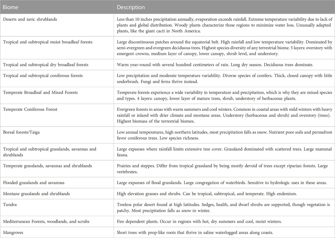
TABLE 1. Global biomes used for analysis and their descriptions, from the WWF (2020).

FIGURE 1

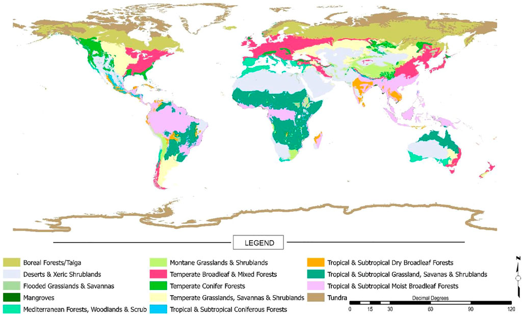
FIGURE 1. Map of the global distribution of the fourteen WWF designated biomes WWF (2020).

Utilizing the length of the satellite data record and the D metric, systematic quantification of vegetation change globally can be derived, and then interpreted with a view to better understand the spatial patterns and trends and how these relate to different global biomes as defined here from the WWF product. Specifically, we will focus on the differences in patterns of vegetation persistence as a function of biome type. Biomes are selected as the broad unit of analysis, as these represent similar ecosystems which, by definition, share comparable processes and major vegetation types wherever they are found. Studying at the level of biomes is important because they may display substantial variation in the extent of change, face different drivers of change, and there may be differences in the options for mitigating or managing these drivers. As such, this research will cover over 30 years of vegetation persistence analysis at the biomes level which is calculated from the global persistence product we created, extracted for each of the 14 biome types. In addition, these biomes are each evaluated at a seasonal scale (DJF, MAM, JJA, and SON) as seasons are something that show different patterns and as such, it is important to both explain and account for these possible phenological signals. Therefore, the created products for analysis and statistical comparison are the persistence patterns for each of the 14 WWF biomes (Table 1; Figure 1) for each of our four seasons, with statistical significance further summarized at a pixel scale and presented for both negative and positive vegetation persistence.

FAO land use diversity data

Information on global land use is of paramount importance within this analysis. Determining biome type does not mean that the land use or land cover matches this type as in many locations land cover change because of changes in land use has already occurred (Winkler et al., 2021; Friedl et al., 2022; Potapov et al., 2022). Therefore, in order to account for the differences as predicted by biomes based on climate and biophysical factors, versus the actual land use, an additional data set was needed. Global data on land use is collected by the Food and Agriculture Organization (FAO) of the United Nations and provides a standardized methodology for land use classification and mapping globally. Given this study was undertaken at a global scale a reputable and readily available global land use data set was needed. The data used for this study was the global land use data product for 2010 which was selected as it related to the end point of the time series used (fao.org website for data download, last accessed September 2022) and so could be used to indicate the actual land use diversity within each biome type. The land use classes available were at a very broad scale and were agriculture, grazing, wetlands, urban, forest, natural non-forest, and open water. The use of the FAO data, allowed us to understand land use diversity within each biome class, where land area within the biome was previously converted, for example, to agricultural or development-based uses, by providing a land use diversity product for 2010. While this data is not ideal, and the time period used was only 2010 it was still useful in interpreting the persistence metrics by biome and by latitude, through a land use diversity analysis, to link to the vegetation dynamics highlighted by the persistence analysis. This allowed us to identify and highlight regions of significant land use diversity, which resulted in the changes in persistence. The data on land use was obtained for the entire globe and then subdivided by biomes, and within each biome was broken down into latitudinal bands, in 10-degree blocks. This was also useful to highlight land use diversity across the northern and southern hemispheres when interpreting the results.

Utilizing the length of the satellite data record and the D metric, systematic quantification of vegetation change globally can be derived, and then interpreted with a view to better understand the spatial patterns and trends and how these relate to land use diversity as calculated here from the FAO product. Specifically, we will focus on the differences in patterns of vegetation persistence as a function of the actual land use diversity at the pixel level, as determined by FAO data (FAO 2010 data available at FAO.org). Biomes are important, but so is land cover and related land use diversity. Therefore, we will calculate the diversity of land uses occurring within each Biomes, and in order to assist interpretation we will calculate this land use diversity for every 10° north and south. This will allow us to add land use diversity into the already complex analysis incorporating biome and season. While this is an added level of complexity, it is essential to highlight the land use diversity within the global biomes data, and how variable this is over the different hemispheres of analysis.

Results

Global patterns of vegetation persistence

We calculated vegetation persistence at a pixel level for each season, for each year, and compared every season/year from 1987 to 2010 to the baseline period of 1982–1986. Initial analysis found AVHRR and MODIS to differ enough that they were not compatible for use within this type of analysis and may impact the findings due to different products and so bias results. Due to these differences across satellite products we chose to utilize the dataset with the longest timeframe and hence selected the AVHRR data product. The results can be evaluated spatially (Figure 2) and an initial review would highlight the overwhelmingly positive pattern of vegetation persistence globally. Despite these overall patterns it is also evident that some regions differ, and negative patterns of vegetation persistence do exist, especially in Africa, and over time, the DFJ or boreal winter experiences more negative persistence patterns. MAM, boreal spring has the most positive patterns of persistence. Such global analysis, while useful, simply provides an overview within which we can start to breakdown findings by biomes and seasons and begin to evaluate potential drivers of these changes.

FIGURE 2

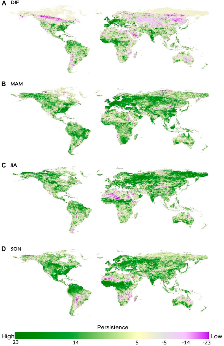
FIGURE 2. Global persistence by season for 1987–2010, compared to the baseline of 1982–1986 for (A) December, January, February (DJF); (B) March, April, May (MAM); (C) June, July, August (JJA); and (D) September, October, November (SON). Positive versus negative trends are shown in green versus purple respectively.

Vegetation persistence patterns by season and biome

Evaluating changes in vegetation persistence by season and biomes provides much more useful data and starts to highlight differences over time and place (Figure 3). For the months DJF there were higher positive trends overall, especially for Tropical Subtropical Moist Broadleaf Forests, Temperate Broadleaf and Mixed Forests, and Tropical Subtropical Grasslands, Savannas and Shrubs (Figure 3A). Two biomes had higher negative persistence patterns over positive patterns, and these were Boreal Forests-Taiga and Temperate Grasslands, Savanna, and Shrublands. The behaviour of these biomes were significantly different for the DJF period, and given their locations may relate in part to data issues related to snow cover at the more northern latitudes recording as low NDVI. As the recorded value is the maximum NDVI in the period this variability with snow cover and snowmelt could result in some erroneous results in terms of vegetation. This also links to the higher areas of negative persistence in the map for DJF (Figure 2A) which helps support this theory.

FIGURE 3

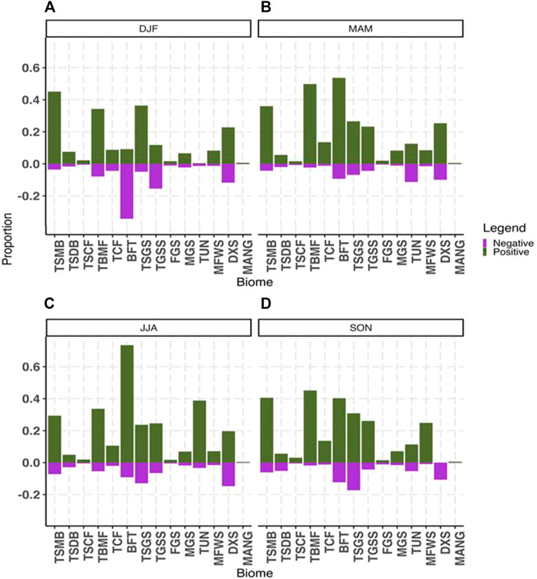
FIGURE 3. Proportion of each biome type globally representing either significant positive vegetation persistence (green) or significant negative vegetation persistence (purple) as a function of total pixels in that biome, and shown for all four seasons for (A) December, January, February (DJF); (B) March, April, May (MAM); (C) June, July, August (JJA); and (D) September, October, November (SON). Where acronyms are: TSMB, Tropical Subtropical Moist Broadleaf Forest; TSDB, Tropical Subtropical Dry Broadleaf Forest; TSCF, Tropical Subtropical Coniferous Forest; TBMF, Temperate Broadleaf and Mixed Forest; TCF, Temperate Coniferous Forest; BFT, Boreal Forests-Taiga; TSGS, Tropical Subtropical Grasslands, Savannas, and Shrublands; TGSS, Temperate Grasslands, Savanna, Shrubland; FGS, Flooded Grassland and Savanna; MGS, Montane Grassland and Shrubland; TUN, Tundra; MFWS, Mediterranean Forest, Woodlands, and Scrub; DXS, Deserts and Xeric Shrublands; and MANG, Mangroves.

For MAM, the results were overwhelmingly positive, with the lowest number of negative pixels for any period. The biomes with the highest numbers of positive persistence values were Boreal Forests/-Taiga, the Temperate Broadleaf and Mixed Forest, and the Tropical Subtropical Moist Broadleaf Forests. The Tundra had equal proportions in negative and positive persistence, all other classes the persistence was dominated by the positive patterns (Figures 2B, 3B). Such an overwhelmingly positive pattern of vegetation persistence in the boreal spring most likely relates to the dominance of the NH in terms of land mass, and the spring season equating to plant growth. Over the time period of study, this indicates that at a pixel level the dominant patterns one of higher NDVI values every year compared to the baseline period, for all biomes except Tundra. This is a real dominance of positive vegetation persistence globally.

During the JJA periods there were overwhelmingly higher positive persistence patterns in every single biome. Again, this likely relates to the growing cycle and the dominance of the NH land mass in the signal. The result of no biomes experiencing more negative persistence versus positive persistence trends though is clearly a major finding. The most significant positive persistence proportions were found in Boreal Forests (with the highest recorded proportion of pixels in the positive persistence class at almost 80%), and then Tundra, Temperate Broadleaf and Mixed Forests, Tundra, Tropical Subtropical Moist Broadleaf Forests, (Figures 2C, 3C).

Finally, for SON there were higher positive persistence patterns again for most classes, although with lower proportions of pixels than for the MAM and JJA periods. The largest proportion of positive persistence was in Temperate Broadleaf and Mixed Forests, followed by Tropical Subtropical Moist Broadleaf Forests and Boreal Forests—Taiga (Figures 2D, 3D). The Deserts and Xeric Shrublands class only record negative persistence patterns and Tropical Subtropical Dry Broadleaf Forests has equal amounts of negative and positive persistence values. As the boreal autumn season occurs then, some of the water-limited or drier environments do appear to have more negative persistence patterns, and the overall greening or vegetative persistence patterns are lower than in the boreal spring and summer periods.

Looking overall at these results, we can view across seasons, and state that positive vegetation persistence is greater in the MAM and JJA seasons (Figures 2, 3) and this likely relates to growing season and more positive vegetation persistence is found in the NH over the SH (Figure 2). Biomes which always have a strong pattern of positive vegetation persistence are the Tropical Subtropical Moist Broadleaf Forests, Temperate Broadleaf and Mixed Forests, and to a lesser degree Tropical Subtropical Grasslands, Savannas and Shrublands. Boreal Forests-Taiga, has very strong patterns of positive vegetation persistence, except for the DJF period, which we believe relates more to snow cover variations than actual land cover. Reviewing these biomes (Figure 1), except for the Argentina pampas grasslands and the tropical subtropical grasslands, savannas and shrublands, these are dominated by the northern hemisphere locations. Overall, it can be seen from the analysis by biomes that forests tend to exhibit more positive patterns of vegetation persistence. Savannas, grasslands and desert regions seem to exhibit much more mixed trends, with more variability intra-annually, or across seasons and hemispheres. From these overview results more information is available and can be extracted to discern any possible drivers of change. As such, the biome data is further broken down, to better understand and explain these trends.

Vegetation persistence patterns accounting for land use diversity within biomes and variation with latitude

Persistence patterns for each biome by latitudinal bands and land use diversity to aid in the analysis and interpretation of the persistence patterns, are illustrated in Figures 4–7. Only those latitudes that represent greater than 5% of the global land surface area of that biome are now included and a vertical grid has been inserted at 33.3% and 66.7% on the significant change bars to provide a rough quantitative estimate of percentages of pixels showing significant positive or negative changes. In addition, each graph also has a right-hand bar chart extended horizontally to accommodate and display the breakdown of land use diversity data in the biome, within each latitudinal band. As such we can interpret the changes in persistence by latitude and discuss each in terms of the actual land use diversity observed within each biome type. This is to account for the land cover changes which have occurred globally, such that a biome has often been converted from its natural vegetation type to more human-dominated uses. This is important to clarify. The biome data represents the vegetation type which would result naturally, but in many cases human driven changes have occurred and the resulting land use is different from the original biome. Therefore, it is essential to highlight that within the biome type the land use diversity is highly variable, emphasizing the alteration that has already occurred within each biome. Clustering of biome types with similar patterns and outcomes can thus be determined and possible reasons for these patterns of change discussed. The patterns of biome responses can be grouped into some similar types where the resulting patterns do appear to follow some similar trends and patterns. To highlight these similar trends in persistence patterns, across seasons, for these biome clusters we have plotted them together (Figures 4D, 5D, 6E, 7E). These graphs show the proportion of pixels in each persistence category (so each biome and season = 100%, similar to soil type triangular charts or “textural triangles”) and plotting by biome across seasons allows us to highlight shifts by season and so link to climatic drivers more effectively.

FIGURE 4

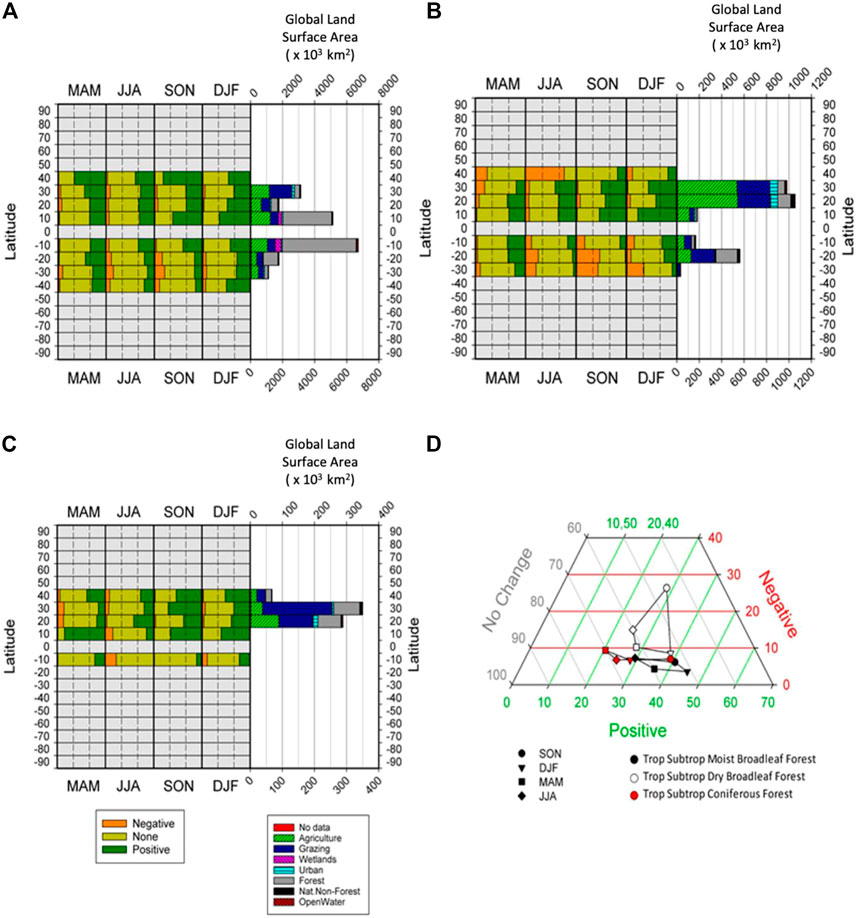
FIGURE 4. Composition of significant persistence values (Negative, None, Positive) in each biome, broken down by latitudinal band, with land use diversity of each bank also shown, for (A) Tropical Subtropical Moist Broadleaf Forest, (B) Tropical Subtropical Dry Broadleaf Forest, (C) Tropical Subtropical Coniferous Forest, and (D) Ternary plot of the seasonal changes in percentages of global areas returning significant percentages of positive and negative persistence, and those reporting to significant persistence, for three tropical forest biomes.

FIGURE 5

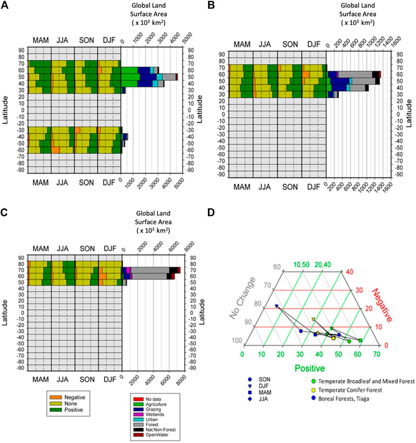
FIGURE 5. Composition of significant persistence values (Negative, None, Positive) in each biome, broken down by latitudinal band, with land use diversity of each bank also shown, for (A) Temperate Broadleaf Mixed Forest, (B) Temperate Coniferous Forest, (C) Boreal Forest -Taiga, and (D) Ternary plot of the seasonal changes in percentages of global areas returning significant percentages of positive and negative persistence, and those reporting to significant persistence, for three non-tropical forest biomes.

FIGURE 6

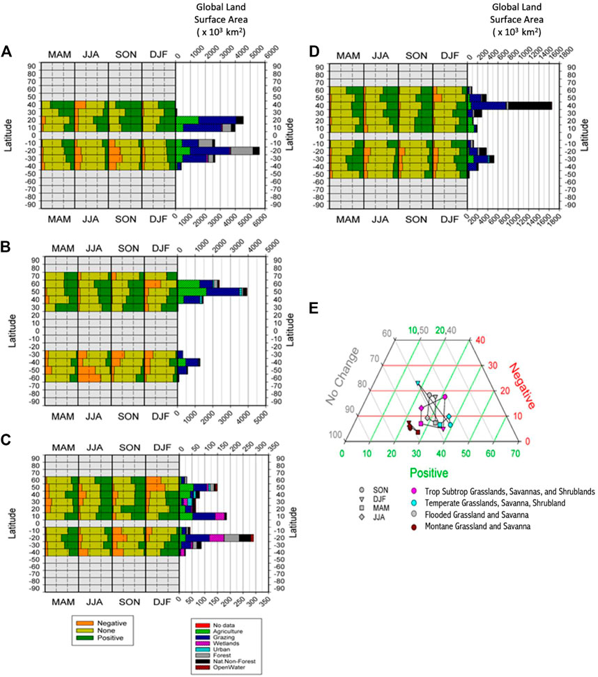
FIGURE 6. Composition of significant persistence values (Negative, None, Positive) in each biome, broken down by latitudinal band, with land use diversity of each bank also shown, for (A) Tropical and Subtropical grasslands, savannas and shrublands, (B) Temperate grasslands, savannas and shrublands, (C) Flooded grasslands and savanna, (D) Montane grassland and shrubland and (E) Ternary plot of the seasonal changes in percentages of global areas returning significant percentages of positive and negative persistence, and those reporting to significant persistence, for four grassland biomes.

FIGURE 7

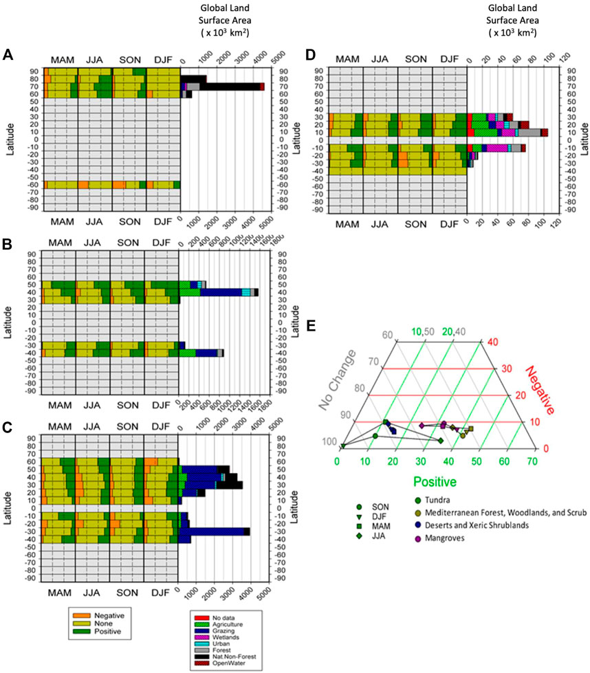
FIGURE 7. Composition of significant persistence values (Negative, None, Positive) in each biome, broken down by latitudinal band, with land use diversity of each bank also shown, for (A) Tundra, (B) Mediterranean Forest, Woodlands and Scrub, (C) Deserts and Xeric Shrublands, (D) Mangroves and (E) Ternary plot of the seasonal changes in percentages of global areas returning significant percentages of positive and negative persistence, and those reporting to significant persistence, for four other biomes.

Tropical Subtropical Moist Broadleaf Forest reveals a significant amount of forest cover is remaining in this biome (Figure 4A) and that the dominant trend is that of positive vegetation persistence. In addition, this trend is clearly stronger in the NH than in the SH. Tropical Subtropical Dry Broadleaf Forest (Figure 4B) has been significantly converted to agriculture and pasture land-uses. The NH shows more positive persistence patterns and for the seasons SON and DJF there is a strong negative trend in the SH. Also, of note, there is more forest cover left in the SH, thus representing more of this original biome cover. Tropical Subtropical Coniferous Forest (Figure 4C) is dominated more by grazing lands, than forest cover along with some agriculture classes.

Positive persistence dominates and this trend is stronger in the NH than the SH, although there is very little SH area in this biome. Figure 4D shows the Tropical and Subtropical Forest types and we can see that Moist Broadleaf and Coniferous Forest types basically run horizontally with very low percentages (5%–10%) of pixels reporting significant negative persistence. By contrast the Tropical and Subtropical Dry Broadleaf Forests show higher percentages of negative persistence in JJA and SON than the other two tropical forest biomes. Given the limiting factors on growth for these biomes, it looks like seasonal availability of moisture may be causing the differences in these three forest types.

Temperate Broadleaf and Mixed Forest (Figure 5A) is now mainly agriculture and grazing lands, with only some limited areas of forest cover left. As with other forest biomes, we find that positive persistence dominates, and this trend is stronger in the NH than the SH. Temperate Coniferous Forest (Figure 5B) has lots of forest cover left, and some limited grazing areas. Again, positive persistence dominates. This biome is only found in the NH and so there is no NH versus SH variability. Boreal Forest-Taiga (Figure 5C) is still predominantly forest cover with much lower rates of conversion and is also found only in the NH. Once again, as with all the forested biome types, positive persistence dominates, especially in the growing season. All non-tropical forest biomes are almost exclusively limited to the NH and display roughly similar shapes, with three triads showing little change in percentages of negative persistence (3%–8%) and DJF (winter) showing the greatest propensity towards negative persistence (Figure 5D). Boreal Forests-Taiga indicate lower percentages (5%–35%) of positive changes, and Temperate Broadleaf and Mixed Forests higher ones (40%–60%). Given limiting factors on growth in these biomes, temperatures seem to have a big role here. In general, cooler temps lead to, a) fewer positive values, b) slightly more negatives (especially DJF), c) more “no significant” and d) a greater amplitude in these observations between the various seasons.

Tropical Subtropical Grasslands, Savannas, Shrublands (Figure 6A) have experienced significant conversion, and are now mainly areas of grazing, with some agriculture. Positive persistence dominates in the NH but the SH is much more variable, with more negative persistence in their winter and spring seasons (JJA and SON respectively). Temperate Grasslands, Savannas, and Shrublands (Figure 6B) have again been mainly transformed to areas of agriculture and grazing. Positive persistence dominates in the NH with the SH again reflecting a more mixed response, with more negative persistence in their winter and spring. Also of note is that these areas are very spatially limited in the SH. Flooded Grassland, and Savanna (Figure 6C) has very mixed actual land uses but despite this, positive persistence dominates in the NH although in the SH results are much more mixed, with more negative persistence in their spring (SON). Montane Grassland and Shrubland (Figure 6D) is composed of mainly grazing and natural vegetation and follows the same trend of positive persistence dominating in the NH, with the SH being a little more mixed, but generally positive overall. Seasonal patterns of persistence for grasslands are very distinct from those of the forest biomes (Figure 6E). The dominant orientation of forest biomes (except tropical dry forest) is horizontal, whereas diagonal (temperate and montane grasslands) and box-like (subtropical and flooded grasslands) shapes dominate here. Flooded grasslands evince greater variability in the vertical position on the graph than tropical grasslands which tend towards a more equilateral shape. From these patterns it seems most likely that they are responding to high seasonality in their rainfall regimes within these grassland biomes.

Tundra (Figure 7A) has mainly natural vegetation cover. Positive persistence dominates in the NH during their growing season. The SH is again much more mixed across seasons although also of note, the SH has very limited area spatially. Mediterranean Forest, Woodlands, and Scrub (Figure 7B) have been heavily converted and so are now mainly agriculture and grazing lands. Positive persistence dominates and this trend is much stronger in the NH than for the SH. Deserts and Xeric Shrublands (Figure 7C) are made up of mainly grazing and natural vegetation. Positive persistence dominates in the NH and following the patterns of many of the grassland and shrub regions, the patterns in the SH are much more variable. Finally, Mangroves (Figure 7D) are greatly transformed and so actually represent very mixed land covers and very small areas. Positive persistence dominates in the NH with the SH more mixed, but with positive persistence overall. Tundra exists almost exclusively in the northern hemisphere, during JJA a high percentage (35%) now exhibit positive persistence, and with very few (<5%) examples of negative persistence (Figure 7D). Between 30% and 40% of the three remaining biomes lie within the southern hemisphere, so what little seasonal variability they exhibit should be interpreted with caution. Regardless of season, just under 80% of the pixels in the desert and xeric shrub biome report no significant persistence and so a discussion of possible drivers of change is not possible.

One important issue here, and a cautionary note on the interpretation of these graphs is related to the fact that any expression and physical interpretation of these changes is partially dependent upon the hemispheric distribution of each biome. As such, it is important to review this percentage of biomes by latitude and hemisphere (Figures 4–8) when reviewing and assigning importance to these results, as we have attempted here.

FIGURE 8

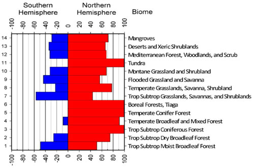
FIGURE 8. Percentage of global biomes by their hemispheric and latitudinal distribution for the 14 biomes under study.

Discussion

This study utilizes a novel approach to analysing NDVI timeseries to better understand global distributions of changes in vegetation greenness. The importance of seasons, biomes, and land use in shaping greenness trajectories was also investigated. This highlighted several advantages and strengths of the directional persistence metric, which utilizes a time series analysis of vegetation persistence, with initial benchmark conditions (1982–1986), and implementing statistical significance at a pixel level for the globe. NDVI time series was shown to be a powerful tool for understanding vegetation change at the global scale. This approach emphasizes identification of long-term shifts in vegetation greenness and is less concerned with small-scale individual events that impact local areas, even though these may be of interest at these more local and regional scales, e.g., forest mortality, disaster related clearing activities, etc. To better capture pixels with significant change in NDVI for individual events, it is possible to adjust the baseline values and temporal scale, though given the global extent of this study it is not possible to account for all local level change in NDVI in the analysis presented here. Future research could look more closely at some areas of interesting change, that do not hit the required significance levels for this research (±9). By using NDVI data to assess the areal extent, magnitude, direction, and temporal patterns of vegetation change, scientists can gain important insights into how vegetation is responding to changes in climate and other environmental conditions, as well as understand the health of ecosystems globally (Southworth et al., 2016; Southworth and Muir 2021).

We calculated vegetation persistence at a pixel level for each season, for each year, and compared every season/year from 1987 to 2010 to the baseline period of 1982–1986. The results highlight the overwhelmingly positive pattern of vegetation persistence globally, although there were also clear regional patterns and variations with season (Figure 2). Looking overall at these results, positive vegetation persistence is greater in the MAM and JJA seasons (Figures 2, 3) and this likely relates to growing season and more positive vegetation persistence as found in the NH over the SH (Figure 2). Overall, forests tend to exhibit more positive patterns of vegetation persistence. Savannas, Grasslands and Desert regions seem to exhibit much more mixed trends, with more variability intra-annually, or across seasons and hemispheres. When broken down further to include land use diversity and latitudinal variation, clearer patterns emerge related to biome types. Tropical Subtropical Moist Broadleaf Forest, Tropical Subtropical Dry Broadleaf and Tropical Subtropical Coniferous Forest have all been heavily converted to agricultural land uses, and the seasonal availability of moisture may be causing the differences in these three forest types (Figure 4). Temperate Broadleaf and Mixed Forest has also been heavily converted to agricultural uses, unlike the Temperate Coniferous Forest Boreal Forest, or Taiga, which are still predominantly intact forest cover. As with all the forested biome types, positive persistence again dominates, especially in the growing season. Given limiting factors on growth in these biomes, temperatures seem to have a big role here in terms of increased patterns of positive vegetation persistence with warmer temperatures (Figure 5). Tropical Subtropical Grasslands, Savannas, Shrublands and Temperate Grasslands, Savannas, and Shrublands have again been largely transformed to areas of agriculture and grazing, whereas Flooded Grassland, and Savanna has very mixed actual land uses. Montane Grassland and Shrubland is composed of mainly grazing and natural vegetation. All follow the same trend of positive persistence dominating in the NH, with the SH being a little more mixed, but generally positive overall. Seasonal patterns of persistence for grasslands are very distinct from those of the forest biomes. From the seasonal patterns and amplitudes (Figure 6) it seems most likely that these grassland biomes are responding to high seasonality in their rainfall regimes. Tundra has mainly natural vegetation cover. Mediterranean Forest, Woodlands, and Scrub and Mangroves have both been heavily converted and so are now mainly agriculture/grazing and mixed covers, and Deserts and Xeric Shrublands are made up of mainly grazing and natural vegetation. Positive persistence dominates in the NH with the SH more mixed, but with positive persistence overall. Variability across these final biome types is high and areal extent often quite small, and no clear patterns or drivers were discernable from the results.

Vegetation persistence (D) is a metric that can be used to understand dynamics and highlight areas of vulnerability based on the patterns of positive and negative vegetation persistence over time. NDVI is a key measure of vegetation health, and by tracking changes in NDVI over time, D can be used to identify areas where vegetation is greening or browning. Positive persistence indicates greening, while negative persistence indicates browning. Areas with high levels of positive persistence are more likely to be resilient to disturbance, while areas with high levels of negative persistence are more vulnerable. By understanding the patterns of vegetation persistence, we can better understand the dynamics of ecosystems and identify areas of possible current or future vulnerability. Over and above that, traditional approaches only highlight the conversion of systems, but “directional persistence,” D, can be used to understand dynamics and highlight areas of vulnerability based on the patterns of positive and negative vegetation persistence over time, as presented here.

This research finds that vegetation persistence exhibited a positive trend overall which matches many of the reports of global greening over the same period (de Jong et al., 2012; 2013; Cortés et al., 2021). Notably, in seasons, positive vegetation persistence is greater in the growing season in the NH. More positive vegetation persistence was found in the NH over the SH, which also corroborates the seasonal and the NH trends exhibited here, and similarly found by other researchers (de Jong et al., 2012; 2013; Cortés et al., 2021). Cortez emphasizes the need for reliable statistically valid tests to detect vegetation change, specifically significant trends related to vegetation greening and browning globally. The research presented here helps validate research finding global greening with much more significant statistical patterns in the NH regions and during the NH growing season, as well as trends of browning, which are much more limited, but found most in the SH. In addition, the importance of land use change and land cover conversions are highlighted and the importance of such land use changes, which are documented as impacting approximately one-third of the global land area since 1960, is critical to incorporate within such studies of global greening or browning (Winkler et al., 2021). The research presented here combines all of these requirements utilizing a well-regarded NDVI vegetation index within a novel and innovative statistical approach, which incorporates mathematical theory to apply statistical significance in a rigorous and repeatable manner, while incorporating season, latitude, and land use diversity. One limitation of this research lies with the use of a single date to develop the land use diversity variable, rather than using multiple dates to determine land use changes. However, the purpose of this research was to focus on the vegetation dynamics represented by the NDVI time-series analysis creating the vegetation persistence metric. Therefore, the use of the single date land use product to create the land use diversity analysis for 2010, to highlight that within each biome type the land use diversity is highly variable, emphasizing the alteration that has already occurred within each biome, is an ideal compromise, within this global focus.

This analysis builds on these previous greening studies of Lu et al. (2016), Piao et al. (2020), Cortés et al. (2021), and Zhu et al. (2016), with the important additions of changes by season, biome, and land use diversity. More regionally and spatially variable, changes in temperature and precipitation, CO₂ fertilization, changes in land cover, and the important role of seasons are all highlighted in these former research studies, as crucial drivers of global greening (vegetation persistence), as can also be observed in the present research. Drivers of global greening from earlier studies, with the key driver being CO₂ fertilization (Lu et al., 2016; Zhu et al., 2016). In the boreal region, temperature change was regarded as the major driver behind vegetation greening as summer facilitated the growth of plants (Lucht et al., 2002), which is in line with findings presented here. But Piao et al. (2005) and Nemani et al. (2002) discovered precipitation as a cause behind enhanced vegetation productivity overall, which again showed congruity with this research, and also highlights the importance of looking within biomes and latitudinal zones, and not just at global trends.

The higher greenness trend in the NH over the SH, is explained by Kaufmann et al. (2002), as rising temperature in the NH as the key factor behind improved vegetation growth. Zhou et al. (2001) and Nemani et al. (2003) also documented enhanced terrestrial greenness in high and middle latitudes of the NH from 1980 to 2000. Box (2002) suggested that because of increased rates of temperate increase in the NH greenness rates are increasing at a higher rate there as compared to the SH. Complimentarily, Piao et al. (2020) suggested that the SH has experienced a wide-ranging trend of greening since 1980, but this rate is lower than compared to higher latitude NH locations. Chen et al. (2019) also regarded the NH as a vegetation greening hotspot because of its faster rates of greening. Winkler et al. (2021) studied sub-Saharan grasslands and savanna systems and showed that the greening pattern is consistent with an increase in rainfall. Zhu et al. (2016) further gave justifications that like climate change, land-use change (deforestation, afforestation, and agricultural intensification) also put forth a highly spatially variable influence on vegetation changes. Deforestation in tropical forests reduced vegetative persistence, described by Brandt et al. (2017), while afforestation increased greenness in the temperate region (Curtis et al., 2018). Additionally, agricultural intensification in terms of irrigation, fertilizer and pesticide use, multiple cropping, etc. contribute significantly (25%–50%) in leaf area enhancement in Mediterranean forest, temperate broadleaf forest, mangroves, and temperate grasslands, as depicted by Feng et al. (2016); Chen et al. (2019), and Winkler et al. (2021). Our research not only supports these same findings but also helps to highlight the latitudinal, seasonal and land use related variations causing these trends.

Conclusion

Vegetation greening is one of the most distinguished characteristics of biosphere change, since 1980, as indicated from long-term satellite records (Lu et al., 2016; Zhu et al., 2016; Piao et al., 2020; Cortés et al., 2021). This study presented an approach to analyzing vegetation persistence for three decades (1982–2010), thus highlighting significant spatial and temporal variations at biome, season and land use diversity levels. By setting 1982–1986 as a benchmark period, the subsequent 23 years of data revealed that forests overall have positive vegetation persistence, but this trend is not consistent across all biomes. Savannas, desert, and grasslands seem to be the most vulnerable although results are highly variable. In contrast, tundra, moist broadleaf forests, boreal forests, and coniferous forests exhibited the highest positive vegetation persistence proportions.

This method in time series remote sensing analysis is pivotal in importance to assist in the user designed, easily replicated, analysis of patterns of vegetation change, which—once identified—can lead to more in-depth and regional scale studies of drivers (Southworth et al., 2016; Southworth and Muir 2021). Vegetation persistence methods, such as the approach in this study, using the vegetation persistence or “D” metric, are much more reproducible and innovative than traditional approaches to vegetation analysis. They take into account patterns of longer-term vegetation persistence, at a pixel level, over extended time periods, rather than just an absolute value. This enables identification of patterns of vegetation change over time, which can then be used to study the drivers of those changes.

This study found similar results to other global studies (de Jong et al., 2012; 2013; Cortés et al., 2021; Jiang et al., 2022), which found an increase in global vegetation persistence since the early 1980s, frequently referred to as the “global greening” trend. However, this study also highlights the importance of exploring these trends across seasons, biomes, and land use diversity, revealing that this trend is not consistent across all locations. Savannas, desert and grasslands seem to be the most vulnerable and highly variable, and forest biomes have the highest patterns of positive vegetation persistence, especially within the growing season. There is a lot of interest in the global greening trend, as it has potential implications for food security, the water cycle and carbon sequestration. However, there is still much work to be done to fully understand the drivers of these trends and their implications. This study provides a valuable contribution to this debate by highlighting the importance of using time series approaches, such as the one presented here, to understand vegetation dynamics and identify areas of vulnerability.

The pixel-level perspective of the vegetation persistence method is useful for understanding dynamics of change and identifying areas of vulnerability. The ability to assign statistical significance to pixel level trajectories helps to further understand the patterns of change. This time series based remote sensing approach has many potential applications for monitoring environmental change. Vegetation persistence, D, can be used to understand dynamics and highlight areas of vulnerability based on the patterns of positive and negative vegetation persistence over time. This can help identify which areas are most likely to experience change and where management action may be necessary to protect against further change. As such, this is a simple and valuable tool for resource managers and policymakers as it provides insight into the long-term impacts of human activities on landscapes.

Data availability statement

The raw data supporting the conclusion of this article will be made available by the authors, without undue reservation.

Author contributions

JS, HH, SR, and EB conceptualized the research, JS, PW, HH, RK, and EB completed analysis, JS, SR, PW, EB, and HH wrote the initial draft, JS, MH, SR, and CM, edited and refined document.

Conflict of interest

The authors declare that the research was conducted in the absence of any commercial or financial relationships that could be construed as a potential conflict of interest.

Publisher’s note

All claims expressed in this article are solely those of the authors and do not necessarily represent those of their affiliated organizations, or those of the publisher, the editors and the reviewers. Any product that may be evaluated in this article, or claim that may be made by its manufacturer, is not guaranteed or endorsed by the publisher.

References

Ahlbeck, J. R. (2002). Comment on “Variations in northern vegetation activity inferred from satellite data of vegetation index during 1981–1999” by L. Zhou et al. J. Geophys. Res. Atmos. 107 (D11), ACH 9-1–ACH 9-2. doi:10.1029/2001jd001389

CrossRef Full Text | Google Scholar

Box, E. O. (2002). Vegetation analogs and differences in the northern and southern hemispheres: A global comparison. Plant Ecol. 163 (2), 139–154. doi:10.1023/A:1020901722992

CrossRef Full Text | Google Scholar

Brandt, M., Rasmussen, K., Peñuelas, J., Tian, F., Schurgers, G., Verger, A., et al. (2017). Human population growth offsets climate-driven increase in woody vegetation in sub-Saharan Africa. Nat. Ecol. Evol. 1 (4), 0081–0086. doi:10.1038/s41559-017-0081

PubMed Abstract | CrossRef Full Text | Google Scholar

Bubenik, P., De Silva, V., and Scott, J. (2015). Metrics for generalized persistence modules. Found. Comput. Math. 15 (6), 1501–1531. doi:10.1007/s10208-014-9229-5

CrossRef Full Text | Google Scholar

Bunting, E. L., Southworth, J., Herrero, H., Ryan, S. J., and Waylen, P. (2018). Understanding long-term savanna vegetation persistence across three drainage basins in Southern Africa. Remote Sens. 10 (7), 1013. doi:10.3390/rs10071013

CrossRef Full Text | Google Scholar

Chen, C., Park, T., Wang, X., Piao, S., Xu, B., Chaturvedi, R. K., et al. (2019). China and India lead in greening of the world through land-use management. Nat. Sustain. 2 (2), 122–129. doi:10.1038/s41893-019-0220-7

PubMed Abstract | CrossRef Full Text | Google Scholar

Corlett, R. T. (2011). Impacts of warming on tropical lowland rainforests. Trends Ecol. Evol. 26 (11), 606–613. doi:10.1016/j.tree.2011.06.015

PubMed Abstract | CrossRef Full Text | Google Scholar

Cortés, J., Mahecha, M. D., Reichstein, M., Myneni, R. B., Chen, C., and Brenning, A. (2021). Where are global vegetation greening and browning trends significant? Geophys. Res. Lett. 48, e2020GL091496. doi:10.1029/2020GL091496

CrossRef Full Text | Google Scholar

Curtis, P. G., Slay, C. M., Harris, N. L., Tyukavina, A., and Hansen, M. C. (2018). Classifying drivers of global forest loss. Science 361 (6407), 1108–1111. doi:10.1126/science.aau3445

PubMed Abstract | CrossRef Full Text | Google Scholar

de Jong, R., Verbesselt, J., Schaepman, M. E., and de Bruin, S. (2012). Trend changes in global greening and browning: Contribution of short-term trends to longer-term change. Glob. Change Biol. 18, 642–655. doi:10.1111/j.1365-2486.2011.02578.x

CrossRef Full Text | Google Scholar

de Jong, R., Verbesselt, J., Zeileis, A., and Schaepman, M. E. (2013). Shifts in global vegetation activity trends. Remote Sens. 5, 1117–1133. doi:10.3390/rs5031117

CrossRef Full Text | Google Scholar

Feng, X., Fu, B., Piao, S., Wang, S., Ciais, P., Zeng, Z., et al. (2016). Revegetation in China’s Loess Plateau is approaching sustainable water resource limits. Nat. Clim. Change 6 (11), 1019–1022. doi:10.1038/nclimate3092

CrossRef Full Text | Google Scholar

Fensholt, R., and Proud, S. R. (2012). Evaluation of Earth observation based global long term vegetation trends—comparing GIMMS and MODIS global NDVI time series. Remote Sens. Environ. 119, 131–147. doi:10.1016/j.rse.2011.12.015

CrossRef Full Text | Google Scholar

Food and Agricultural Organization of the United Nations (2010). Data available via https://www.fao.org/faostat/en/#data/RL. Last accessed September 1 2022.

Friedl, M. A., Woodcock, C. E., Olofsson, P., Zhu, Z., Loveland, T., Stanimirova, R., et al. (2022). Medium spatial resolution mapping of global land cover and land cover change across multiple decades from landsat. Front. Remote Sens. 3, 894571. doi:10.3389/frsen.2022.894571

CrossRef Full Text | Google Scholar

Gómez, C., White, J. C., and Wulder, M. A. (2016). Optical remotely sensed time series data for land cover classification: A review. ISPRS J. Photogrammetry Remote Sens. 116, 55–72. doi:10.1016/j.isprsjprs.2016.03.008

CrossRef Full Text | Google Scholar

Herrmann, S. M., Anyamba, A., and Tucker, C. J. (2005). Recent trends in vegetation dynamics in the African Sahel and their relationship to climate. Glob. Environ. Change 15 (4), 394–404. doi:10.1016/j.gloenvcha.2005.08.004

CrossRef Full Text | Google Scholar

Jiang, F., Deng, M., Long, Y., and Sun, H. (2022). Spatial pattern and dynamic change of vegetation greenness from 2001 to 2020 in tibet, China. Front. Plant Sci. 13, 892625. doi:10.3389/fpls.2022.892625

PubMed Abstract | CrossRef Full Text | Google Scholar

Kaufmann, R. K., Zhou, L., Tucker, C. J., Slayback, D., Shabanov, N. V., and Myneni, R. B. (2002). Reply to Comment on ‘Variations in northern vegetation activity inferred from satellite data of vegetation index during 1981–1999 by JR Ahlbeck. J. Geophys. Res. 107 (4127), ACL 7-1–ACL 7-3. doi:10.1029/2001jd001516

CrossRef Full Text | Google Scholar

Keenan, T. F., and Riley, W. J. (2018). Greening of the land surface in the world’s cold regions consistent with recent warming. Nat. Clim. change 8 (9), 825–828. doi:10.1038/s41558-018-0258-y

PubMed Abstract | CrossRef Full Text | Google Scholar

Lanfredi, M., Simoniello, T., and Macchiato, M. (2004). Temporal persistence in vegetation cover changes observed from satellite: Development of an estimation procedure in the test site of the Mediterranean Italy. Remote Sens. Environ. 93 (4), 565–576. doi:10.1016/j.rse.2004.08.012

CrossRef Full Text | Google Scholar

Lenka, N. K., and Lal, R. (2012). Soil-related constraints to the carbon dioxide fertilization effect. Crit. Rev. Plant Sci. 31 (4), 342–357. doi:10.1080/07352689.2012.674461

CrossRef Full Text | Google Scholar

Liu, H., Jiao, F., Yin, J., Li, T., Gong, H., Wang, Z., et al. (2020). Nonlinear relationship of vegetation greening with nature and human factors and its forecast–a case study of Southwest China. Ecol. Indic. 111, 106009. doi:10.1016/j.ecolind.2019.106009

CrossRef Full Text | Google Scholar

Liu, Y., Chai, Y., Yue, Y., Huang, Y., Yang, Y., Zhu, B., et al. (2022). Effects of global greening phenomenon on water sustainability. CATENA 208, 105732. doi:10.1016/j.catena.2021.105732

CrossRef Full Text | Google Scholar

Lu, X., Wang, L., and McCabe, M. F. (2016). Elevated CO2 as a driver of global dryland greening. Sci. Rep. 6 (1), 20716–20717. doi:10.1038/srep20716

PubMed Abstract | CrossRef Full Text | Google Scholar

Lucht, W., Prentice, I. C., Myneni, R. B., Sitch, S., Friedlingstein, P., Cramer, W., et al. (2002). Climatic control of the high-latitude vegetation greening trend and Pinatubo effect. Science 296 (5573), 1687–1689. doi:10.1126/science.1071828

PubMed Abstract | CrossRef Full Text | Google Scholar

Lunetta, R. S., Knight, J. F., Ediriwickrema, J., Lyon, J. G., and Worthy, L. D. (2006). Land-cover change detection using multi-temporal MODIS NDVI data. Remote Sens. Environ. 105 (2), 142–154. doi:10.1016/j.rse.2006.06.018

CrossRef Full Text | Google Scholar

Marshall, E., Valavi, R., Connor, L. O., Cadenhead, N., Southwell, D., Wintle, B. A., et al. (2021). Quantifying the impact of vegetation-based metrics on species persistence when choosing offsets for habitat destruction. Conserv. Biol. 35 (2), 567–577. doi:10.1111/cobi.13600

PubMed Abstract | CrossRef Full Text | Google Scholar

Nemani, R., and Running, S. (1997). Land cover characterization using multitemporal red, near-IR, and thermal-IR data from NOAA/AVHRR. Ecological applications 7 (1), 79–90.

CrossRef Full Text | Google Scholar

Nemani, R. R., Keeling, C. D., Hashimoto, H., Jolly, W. M., Piper, S. C., Tucker, C. J., et al. (2003). Climate-driven increases in global terrestrial net primary production from 1982 to 1999. Science 300 (5625), 1560–1563. doi:10.1126/science.1082750

PubMed Abstract | CrossRef Full Text | Google Scholar

Nemani, R., White, M., Thornton, P., Nishida, K., Reddy, S., Jenkins, J., et al. (2002). Recent trends in hydrologic balance have enhanced the terrestrial carbon sink in the United States. Geophys. Res. Lett. 29 (10), 106-1–106-4. doi:10.1029/2002gl014867

CrossRef Full Text | Google Scholar

Olson, D. M., Dinerstein, E., Wikramanayake, E. D., Burgess, N. D., Powell, G. V. N., and Underwood, E. C. (2001). Terrestrial ecoregions of the world: A new map of life on Earth. Bioscience 51 (11), 933–938.

CrossRef Full Text | Google Scholar

Piao, S., Fang, J., Zhou, L., Zhu, B., Tan, K., and Tao, S. (2005). Changes in vegetation net primary productivity from 1982 to 1999 in China. Glob. Biogeochem. Cycles 19 (2). doi:10.1029/2004gb002274

CrossRef Full Text | Google Scholar

Piao, S., Friedlingstein, P., Ciais, P., Zhou, L., and Chen, A. (2006). Effect of climate and CO2 changes on the greening of the Northern Hemisphere over the past two decades. Geophys. Res. Lett. 33 (23), L23402. doi:10.1029/2006gl028205

CrossRef Full Text | Google Scholar

Piao, S., Wang, X., Park, T., Chen, C., Lian, X. U., He, Y., et al. (2020). Characteristics, drivers and feedbacks of global greening. Nat. Rev. Earth Environ. 1 (1), 14–27. doi:10.1038/s43017-019-0001-x

CrossRef Full Text | Google Scholar

Potapov, P., Hansen, M. C., Pickens, A., Hernandez-Serna, A., Tyukavina, A., Turubanova, S., et al. (2022). The global 2000-2020 land cover and land use change dataset derived from the landsat archive: First results. Front. Remote Sens. 3, 856903. doi:10.3389/frsen.2022.856903

CrossRef Full Text | Google Scholar

Samanta, A., Ganguly, S., Hashimoto, H., Devadiga, S., Vermote, E., Knyazikhin, Y., et al. (2010). Amazon forests did not green-up during the 2005 drought. Geophys. Res. Lett. 37 (5). doi:10.1029/2009gl042154

CrossRef Full Text | Google Scholar

Southworth, J., and Muir, C. (2021). Specialty grand challenge: Remote sensing time series analysis. Front. Remote Sens. 2, 770431. doi:10.3389/frsen.2021.770431

CrossRef Full Text | Google Scholar

Southworth, J., Zhu, L., Bunting, E., Ryan, S. J., Herrero, H., Waylen, P. R., et al. (2016). Changes in vegetation persistence across global savanna landscapes, 1982–2010. J. Land Use Sci. 11 (1), 7–32. doi:10.1080/1747423X.2015.1071439

CrossRef Full Text | Google Scholar

Tian, F., Liu, L. Z., Yang, J. H., and Wu, J. J. (2021). Vegetation greening in more than 94% of the Yellow River Basin (YRB) region in China during the 21st century caused jointly by warming and anthropogenic activities. Ecol. Indic. 125, 107479. doi:10.1016/j.ecolind.2021.107479

CrossRef Full Text | Google Scholar

Tsai, H., Southworth, J., and Waylen, P. (2014). Spatial persistence and temporal patterns in vegetation cover across Florida, 1982–2006. Phys. Geogr. 35 (2), 151–180. doi:10.1080/02723646.2014.898126

CrossRef Full Text | Google Scholar

Wang, X., Dannenberg, M. P., Yan, D., Jones, M. O., Kimball, J. S., Moore, D. J., et al. (2020). Globally consistent patterns of asynchrony in vegetation phenology derived from optical, microwave, and fluorescence satellite data. J. Geophys. Res. Biogeosciences 125 (7), e2020JG005732. doi:10.1029/2020jg005732

CrossRef Full Text | Google Scholar

Washington-Allen, R. A., West, N. E., Ramsey, R. D., and Efroymson, R. A. (2006). A protocol for retrospective remote sensing–based ecological monitoring of rangelands. Rangel. Ecol. Manag. 59 (1), 19–29. doi:10.2458/azu_jrm_v59i1_allen

CrossRef Full Text | Google Scholar

Waylen, P., Southworth, J., Gibbes, C., and Tsai, H. (2014). Time series analysis of land cover change: Developing statistical tools to determine significance of land cover changes in persistence analyses. Remote Sens. 6 (5), 4473–4497. doi:10.3390/rs6054473

CrossRef Full Text | Google Scholar

Wilson, A. G., and Kirkby, M. J. (1980). Mathematics for Geographers and Planners. 2nd Edn. Oxford, United Kingdom: Oxford University Press.

Winkler, A. J., Myneni, R. B., Hannart, A., Sitch, S., Haverd, V., Lombardozzi, D., et al. (2021). Slowdown of the greening trend in natural vegetation with further rise in atmospheric CO₂ Biogeosciences 18 (17), 4985–5010. doi:10.5194/bg-18-4985-2021

CrossRef Full Text | Google Scholar

Winkler, K., Fuchs, R., Rounsevell, M., and Herold, M. (2021). Global land use changes are four times greater than previously estimated. Nat. Commun. 12, 2501. doi:10.1038/s41467-021-22702-2

PubMed Abstract | CrossRef Full Text | Google Scholar

Xiao, J., and Moody, A. (2005). A comparison of methods for estimating fractional green vegetation cover within a desert-to-upland transition zone in central New Mexico, USA. Remote Sens. Environ. 98 (2–3), 237–250. doi:10.1016/j.rse.2005.07.011

CrossRef Full Text | Google Scholar

Yao, R., Wang, L., Huang, X., Chen, X., and Liu, Z. (2019). Increased spatial heterogeneity in vegetation greenness due to vegetation greening in mainland China. Ecol. Indic. 99, 240–250. doi:10.1016/j.ecolind.2018.12.039

CrossRef Full Text | Google Scholar

Zhao, M., and Running, S. (2010). Drought-induced reduction in global terrestrial net primary production from 2000 through 2009. Science 329 (5995), 940–943. doi:10.1126/science.1192666

PubMed Abstract | CrossRef Full Text | Google Scholar

Zhou, L., Tucker, C. J., Kaufmann, R. K., Slayback, D., Shabanov, N. V., and Myneni, R. B. (2001). Variations in northern vegetation activity inferred from satellite data of vegetation index during 1981 to 1999. J. Geophys. Res. Atmos. 106 (D17), 20069–20083. doi:10.1029/2000jd000115

CrossRef Full Text | Google Scholar

Zhu, Z., Piao, S., Myneni, R. B., Huang, M., Zeng, Z., Canadell, J. G., et al. (2016). Greening of the earth and its drivers. Nat. Clim. change 6 (8), 791–795. doi:10.1038/nclimate3004

CrossRef Full Text | Google Scholar