An integrated hierarchical classification and machine learning approach for mapping land use and land cover in complex social-ecological systems

1 Introduction

Land use and land cover (LULC) mapping characterize the anthropogenic influences and natural elements that occupy a landscape at a specific time based on established methods and appropriate data sources (Nedd et al., 2021). Land use ranks among the important environmental factors that affect natural and socio-economic systems at local, regional and global levels (Lambin et al., 2003; Bajocco et al., 2012; IPBES, 2018; Vijith et al., 2018; Jung et al., 2019). It affects vegetation cover that underpins terrestrial ecosystem functions (Anderson et al., 1976; Yesuph and Dagnew, 2019) and influences human wellbeing (IPBES, 2018; IPBES, 2019). However, the contemporary unprecedented rate of LULC change is troubling (Meiyappan et al., 2014; Showqi et al., 2014), with model projections suggesting it will likely continue manifesting overwhelming impacts even by 2,100 (Sala et al., 2000). Consequently, an urgent need exists to produce detailed and accurate LULC maps to advance our understanding of the causes and putative drivers of change to guide implementation of potential mitigation measures (Hansen et al., 2000; IPBES, 2019). This is especially relevant for complex landscapes with gradual transitions between LULC categories, such as grasslands, woody grasslands, woodlands and forests as found in the African savannas, where LULC change impacts are profound yet poorly understood (Reed et al., 2009; Homewood et al., 2012). This poor understanding stems from both the technical difficulty of classifying their LULC categories given their inherent complexity and the fine grain of underlying socio-ecological processes that drive the changes.

Mapping LULC is an operational source of information for many sectors such as environmental impacts reporting, biodiversity conservation and food security assessment (Serneels and Lambin, 2001; Lambin et al., 2003; Reed et al., 2009; Shiferaw et al., 2011). It is essential for guiding integrated spatial planning and tackling environmental, socio-economic and political challenges beyond traditional management boundaries (Reed and Curzon, 2015). Consequently, many LULC maps have been derived from ground observations and remotely sensed data (Loveland et al., 2000; Pandey et al., 2021), however, producing accurate and consistently classified maps for heterogeneous and complex landscapes such as savannas is exceedingly challenging (Loveland et al., 2000; Hansen et al., 2013). The limitations are due largely to lack of good coverage, using few ground-truthing samples (Krig, 2014), ambiguous or narrow classification schemes (DiGregorio and Jansen, 2000), and inefficient analytical tools, and non-robust classifiers stemming from the inherently fuzzy nature of the LULC categories. Costly software and algorithms further make it difficult to obtain the best available tools for image processing and analysis.

The quality of LULC maps strongly depends upon the clarity and quality of remote sensing images and varies with the spatial resolution of sensors (Xie et al., 2008) and multiple biotic and abiotic factors. The latter include climatic (atmospheric) effects, topography, land cover heterogeneity and plant growth stages (Loveland et al., 2000; Hansen et al., 2013). Image clarity depends on the spatial resolution of satellite sensors such that high-resolution images have finer and clearer pixels than medium to coarse-resolution images because of averaging over less spatial heterogeneity (Xie et al., 2008). Atmospheric effects can degrade images by scattering solar radiation through constituent gasses and aerosols (Chavez, 1996; Tyagi and Bhosle, 2011), cloud cover causes opaque surfaces, whereas rugged or undulating terrain will cast shadows on parts of land cover type (Sun et al., 2018). Further, the size of a study area and its topography can make fieldwork very strenuous and expensive (i.e., budgetary and time constraints), and possibly lead to the collection of too few ground-truthing samples during fieldwork. However, several strategies can be used to overcome the challenges in LULC mapping from remotely sensed data. 1) Selection of clear images for analysis, i.e., free of cloudiness and haze as much as possible. 2) Many training and validation samples to improve model fit and predictive accuracy (Congalton, 1991; Wu and Shapiro, 2006). 3) Use of pre-existing auxiliary data and well-trained teams with sufficient socio-ecological knowledge to aid the classification and extraction of thematic features (Shrestha and Zinck, 2001; Gad and Kusky, 2006). 4) Stratification of the landscapes into smaller zones with greater ecological similarity and inherent land use change narratives to minimize the spread of spectral signatures during image processing (Smith et al., 2003; Hansen et al., 2013; Sleeter et al., 2013). 5) Well-tested and standardized classification systems. 6) Robust classifiers and analytical tools (Breiman, 2001; Janitza and Hornung, 2018).

Various machine learning and other classifiers are widely used for modeling LULC types in remote sensing image detection and visualization, pattern recognition, classification, fusion and object-based analysis (Hussain et al., 2013). Efficient classifiers include random forest (Breiman, 2001), soft or fuzzy classifiers (Binaghi et al., 1999; Ralescu and Visa, 2011), support vector machines (Taati et al., 2015), deep learning (Ma et al., 2019; Li et al., 2020a; Li et al., 2020b, boosting algorithms (Ghimire et al., 2012), object-oriented classifiers (Zhao et al., 2020), spectral unmixing (Keshava and Mustard, 2002), classifiers based on texture measures (Raju and Durai, 2013; Cavalin and Oliveira, 2017) and decision-tree and rule-based classifiers (Berhane et al., 2018).

We selected the RF classifier for this study because of its excellent predictive performance and computational efficiency with high-dimensional data (Janitza and Hornung, 2018). The RF is increasingly being used as a classifier of choice for LULC classification of remotely sensed data (e.g., Gislason et al., 2006; Belgiu and Drăguţ, 2016; Thi et al., 2019). The RF is a refinement of ensemble machine learning methods for reducing prediction variance using recursive binary partitioning and bootstrap aggregation (Breiman, 2001). These include bagging if random subsamples are drawn from a training dataset with replacement to create an ensemble of training samples and sub-bagging if the random subsamples are taken from the training dataset without replacement. The predictions in classification are typically based on a majority vote and are aggregated across trees using means (bagging) or medians (bragging). Random subsampling with replacement and averaging over trees produces stable fitted values and reduces overfitting and prediction variance whereas randomly selecting subsets of predictors without replacement to split each tree node increases the independence of predictions across trees. RF can also perform both classification and regression, produce partial dependence plots for multi-category classes and rank predictor variables in order of their importance (Kotsiantis, 2010; Belgiu and Drăguţ, 2016).

The predictive performance of the RF can be evaluated using an error estimate computed from the out-of-bag (OOB) data. The OOB error is an unbiased estimator of the true error rate of the RF, and also measures the prediction error of other related methods that use bootstrap aggregation such as boosted decision trees (Zhang et al., 2010; Janitza and Hornung, 2018). The RF uses all the original samples to construct the classifier and estimate the OOB error and saves storage and processing time for high-dimensional data (Janitza and Hornung, 2018). However, the RF classifier has some shortcomings too, including inefficient error estimation with k-fold cross-validation and other data-splitting approaches that leave out a subset of the sample (Bylander, 2002; Zhang et al., 2010).

Several alternative approaches have been explored for mapping LULC within the Extended Greater Masai Mara Ecosystem (EGMME) of southwestern Kenya (Betts, 1953; Trapnell et al., 1969; Glover and Trump, 1970; Epp and Agatsiva, 1980; Mwichabe, 1986; Karime, 1990; Mundia and Murayama, 2009; Reed et al., 2009; Mireille et al., 2019; Supplementary Table S7). However, none of these has so far produced detailed and reliable maps of the structural vegetation heterogeneity and density and anthropogenic land use with a consistent classification at the local to larger scales. More precisely, to our knowledge, no method exists for producing accurate, consistent and detailed LULC maps at landscape to regional and continental scales from fine to medium-resolution images, especially for complex landscapes with gradual transitions between LULC categories such as African savannas. Yet, an approach for describing the fine to general characteristics and composition of vegetation cover is essential for understanding environmental changes and linking them to putative drivers (Veldhuis et al., 2019).

We propose a new, reliable, flexible and general approach for mapping detailed to general structural vegetation heterogeneity and density and anthropogenic land use in complex socio-ecological systems such as African savannas. The method integrates a well-tested and hierarchical vegetation classification system with a robust machine learning (RF) classifier and is illustrated using landscape stratification and extensive training and ground-truthing sites to evaluate its classification accuracy. We implement the approach and evaluate its predictive performance for a premier East African savanna ecosystem, the Extended Greater Masai Mara Ecosystem (EGMME). The EGMME is an ideal test bed for our approach because its landscape is expansive and highly heterogeneous.

We adopt a well-tested hierarchical vegetation classification system (Grunblatt et al., 1989) developed for multiple land cover types from multiple data sources (ground observation, aerial and satellite data) and extend it to incorporate anthropogenic land use (specifically cropland and built-up areas) and water bodies. We stratify the landscape into zones to account for spatial heterogeneity and optimise the selection of training and ground-truthing samples, therefore enhancing prediction accuracy to ensure local relevance of the cover classes. We illustrate the approach using large training and ground-truthing datasets. We evaluate the accuracy of visual image classification using discrete matching, assess the overall and class-specific accuracies and computational efficiency of the RF classifier with and without stratification, and compare our findings with those of previous studies in the same landscape. The approach is general, reproducible and versatile, yields consistent classification with high accuracy and can be used in various applications including spatial planning, habitat suitability assessment and change detection.

2 Materials and methods

2.1 Study area

We conducted the study in the Extended Greater Masai Mara ecosystem (EGMME), a vast and complex savanna, occupying 11259.4 km² in southwestern Kenya (Figure 1). The study area covers 65% of the Mara River Basin (MRB, 8,938 km²) and the overlapping Greater Masai Mara Ecosystem (GMME, 7,500 km²; Stelfox et al., 1986). The remaining 35% of the MRB is located across the northern Serengeti National Park and extends into Lake Victoria in Tanzania. The GMME is defined by the historic range of wildebeest migration and encompasses the Masai Mara National Reserve (MMNR, 1,530 km²), the adjacent wildlife conservancies (created from 2005 to 2006) and unregulated pastoral lands (Stelfox et al., 1986; Bhola et al., 2012; Bedelian and Ogutu, 2017). The MME has diverse vegetation communities and land uses including traditional pastoralism, ranching, conservation, forestry and crop production. It is home mainly to Maasai people and their livestock but also hosts diverse wildlife assemblages (Homewood et al., 2012; Ogutu et al., 2016; Løvschal et al., 2019).

FIGURE 1

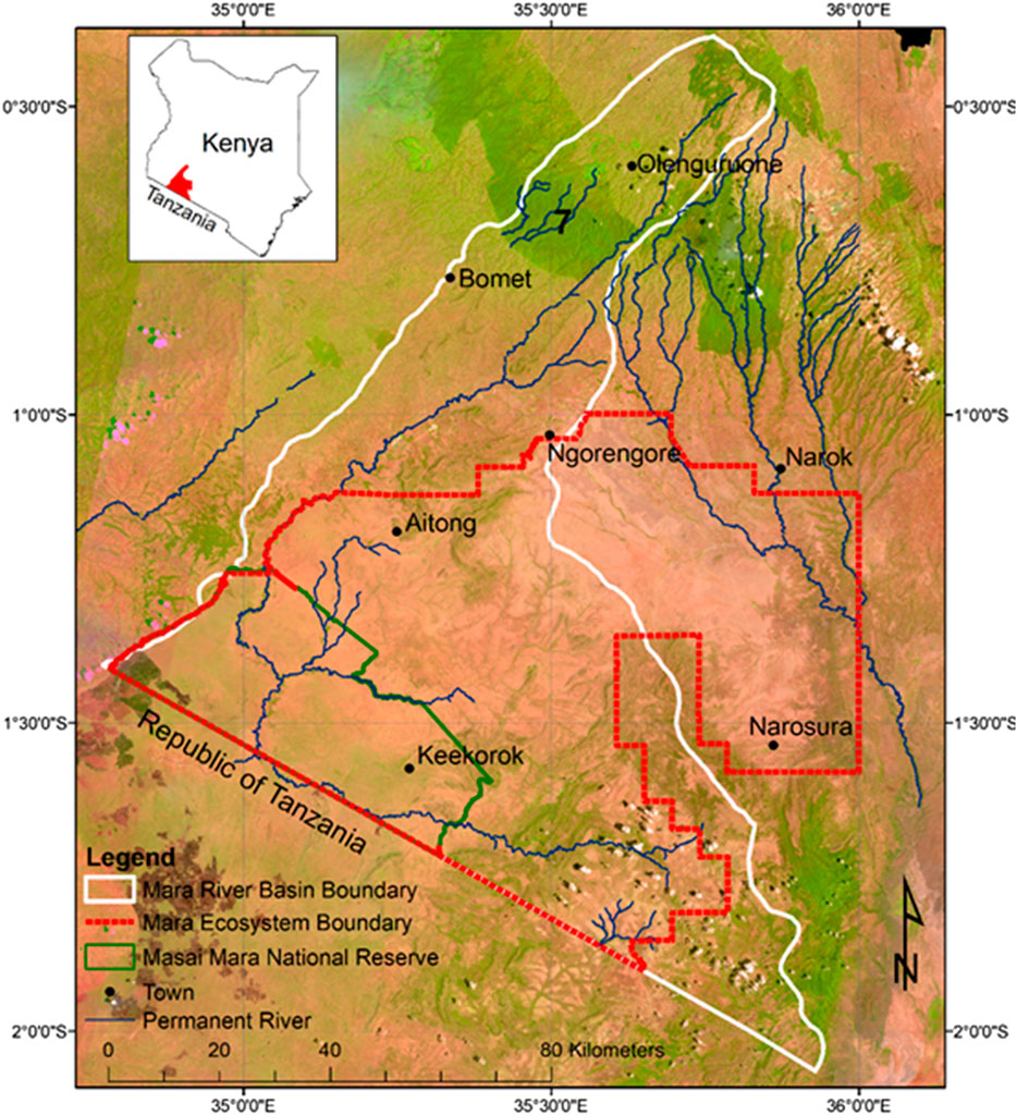
FIGURE 1. The Extended Greater Masai Mara Ecosystem (EGMME) encompasses part of the Mara River Basin in Kenya (white thick outline) and the entire Greater Masai Mara Ecosystem (GMME, red dotted outline) (Stelfox et al., 1986) that largely overlap. Background: Landsat 8 OLI multispectral image for February 2015.

The MME is generally covered by grassland, shrubland, woodland and cultivated areas. It contains one of Kenya’s major “water towers” (upland river catchment areas, Mau Forest Complex in this case), wildlife biodiversity ‘hotspots’ (MMNR and its neighbouring conservancies) and is bordered in the south by the Tanzanian Serengeti National Park (SNP) (Veldhuis et al., 2019).

In recent decades, the MME has experienced rapid LULC changes due to human population growth, land tenure privatization and land subdivision (Bedelian and Ogutu, 2017; Nkedianye et al., 2020) and expansion of cultivation and settlements (Serneels and Lambin, 2001; Lamprey and Reid, 2004) compounded by widening climatic variability (Bartzke et al., 2018). Cropland, supporting small-scale rainfed cultivation and livestock keeping (crop-livestock system) are widespread in the wetter Mau upland and footslopes. Large-scale (wheat and maize) fields have progressively expanded into the transitional zone in the lowland (Karime, 1990; Serneels and Lambin, 2001; Lamprey and Reid, 2004).

Rainfall in the MME is bimodal and increases up a gradient from the southeast (ca. 600 mm/year) to the northwest (ca. 1,300 mm/year), east to west and south to north (Norton-Griffiths et al., 1975; Bartzke et al., 2018; Mukhopadhyay et al., 2019). The Mara River, the only permanent river and lifeline of the whole Serengeti-Mara ecosystem in dry periods, originates in the Mau uplands at Napuiyapi swamp (2,932 m a.s.l). Several of its tributaries traverse the Mara plains before converging onto the Mara River in the Masai Mara Reserve and draining into Lake Victoria through the SNP.

2.1.1 Data sources and types

The EGMME is covered by two Landsat 8 images, path/row 169/60 and 169/61. We downloaded the two images acquired on the 13th and 15th February 2015 from the USGS portal (https://earthexplorer.usgs.gov/). The images were already radiometrically calibrated, orthorectified, geometrically corrected and projected on the WGS (1984) Universal Transverse Mercator (UTM) zone 36S from the source.

These images were acquired during a short dry period after the early wet season from December to January, the best time of year to obtain clear scenes from space in this equatorial region because the short rains remove dust from the air making LULC differences clearer, cultivation has just started and vegetation has greened up (Reed et al., 2009; Kija et al., 2020). The images had <5% cloudiness and were haze-free as much as possible. Furthermore, the cropland can be distinguished from natural vegetation in the medium-resolution images during the post-harvest period, whereas active vegetation growth in the wet season emits a combination of spectral reflectances, making them harder to discriminate, while the cloudiness may also obscure large areas (Xie et al., 2008).

Several ancillary data were used to aid the visual image interpretation and extraction of thematic features (Shrestha and Zinck, 2001; Gad and Kusky, 2006). 1) High-resolution Google Earth Pro and aerial photos taken around the time of image acquisition by Kenya’s Directorate of Resource Surveys and Remote Sensing (DRSRS). 2) Road network and urban/rural settlements from Kenya’s Ministry of Roads and Physical Planning. The road network was used for orientation and to create buffers to select the ground-truthing sites. 3) A digital elevation model (DEM, Shuttle Radar Topography Mission, 30 m) was used in the ‘C’ correction method for normalizing the cast shadows over rugged terrains. 4) Agro-ecological zones for demarcation of potential crop areas and rainfall regimes (https://infonet-biovision.org/). 5) Physical boundary of the protected areas (wildlife and forest reserves and conservancies) from the Kenya Wildlife Service (KWS) and the Maasai Mara Wildlife Conservancies Association (MMWCA). 6) DRSRS 5 × 5 km permanent grid for assessing large herbivore population (Ogutu et al., 2016), land use and habitat conditions in the Kenya rangelands using the Grunblatt et al. (1989) classification system. 7) Human population density from the Kenya National Bureau of Statistics (KNBS) for evaluating land use intensity. 8) Expert socio-ecological knowledge of the study landscape.

2.1.2 Image preprocessing

A schematic illustration of the general steps in our approach is provided in Figure 2. First, we prepared the images to ensure greater clarity and quality before stratifying the landscape and undertaking the visual image classification. Landsat 8 has eight spectral bands (1–7) and band 9 at 30 m spatial resolution, panchromatic (band 8) at 15 m and thermal infrared (bands 10 and 11) at 100 m. Bands 2–5 emphasise the peak vegetation cover used to assess plant vigour, soils and biomass content; bands 6 and 7 discriminate vegetation and soil moisture content and band 9 detect cirrus cloud contamination. We used bands 2-7 and 9 to create the multispectral composite image in ENVI 5.3.1 but did not use bands 1 (coastal aerosol), 8, 10 and 11 because they were unsuitable for our purpose.

FIGURE 2

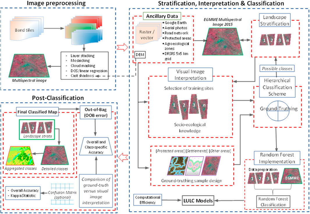
FIGURE 2. A diagrammatic illustration of the LULC classification process showing each module represented by a dashed box and described in the text.

We followed the five general steps outlined below.

i) The seven bands for each scene were layer-stacked to a multiband. tif file composite in ENVI 5.3.1. This image was visualized both as an RGB composite (bands 4, 3, 2) and a false color composite (bands 5, 4, 3). All seven bands were used for the RF classification. The two images were combined by histogram matching for each band, then seamlessly merged into a single multispectral image.

ii) A few clouds dotted a small section of the study area, particularly in the Mau upland. We zoomed into the clouded area and extracted the pixels with clouds on the image using the Fmask tool in ENVI 5.3.1, then refilled the gaps with similar pixels from a cloud-free image spaced maximally 64 days apart. We corrected the atmospheric effects between the original image and the new pixels inserted using the QUick Atmospheric Correction (QUAC) tool (Zhu et al., 2018)

iii) To correct for atmospheric effects that can cause false indications of objects on the image, we used the Dark Object Subtraction (DOS) and linear regression methods (Franklin and Giles, 1995; Chavez, 1996) in QGIS 3.2 (QGIS Development Team, 2019). This procedure removes inconsistency of image brightness by reducing values to provide the ‘true’ surface reflectances. It normalizes the difference within and between the images and the sensor by converting the pixel brightness value (DN) to the actual ground reflectance (Top-of-Atmosphere) value (Gilabert et al., 1994).

iv) The merged boundaries of the Mara River Basin (MRB) and the Greater Masai Mara Ecosystem (GMME) using ArcGIS vers. 10.5 (ESRI, 2016a) demarcated the extent of the EGMME. We created a 10-km buffer around the EGMME boundary and masked the pixels outside this area by assigning them no data.

v) Relief elevation and rugged terrains are common features of the study landscape and often cast shadows on some parts of the land cover due to obstruction of direct solar radiation or illumination. We normalized the displayed reflectance values on the shadowed parts of the same cover type using the ‘C’ correction method (an automated algorithm combining a 30-m digital elevation model (DEM). The procedure compensates for radiance that affects illumination conditions (Giles, 2001; Suriyaprasita and Shrestha, 2008). Then, we applied a 3 × 3-pixel kernel convolution to characterize and sharpen image objects by embossing features to stand out (i.e., different cover types respond differentially to slope and illumination effects) (Ekstrand, 1996; Amro et al., 2011).

2.1.3 Stratification of the EGMME into zones

The stratification of complex landscapes is important for image interpretation because it enables their delineation into relatively internally homogeneous areas for qualitative evaluation. Moreover, it reduces the variance of the parameter estimates and predictions of quantitative variables, thereby improving accuracy (Ndao et al., 2021). Our study landscape is characterised by remarkable variations in geomorphology, topography, climatic and protection status, land tenure change and human population growth, which greatly influence LULC (Wubie et al., 2016). Consequently, we used these factors together with agroecological zones and inferred image patterns to partition the EGMME into eight internally more homogeneous and ecologically similar zones (Loveland and Merchant, 2004; Sleeter et al., 2013). More detailed descriptions of each zone are provided in Table 1.

TABLE 1

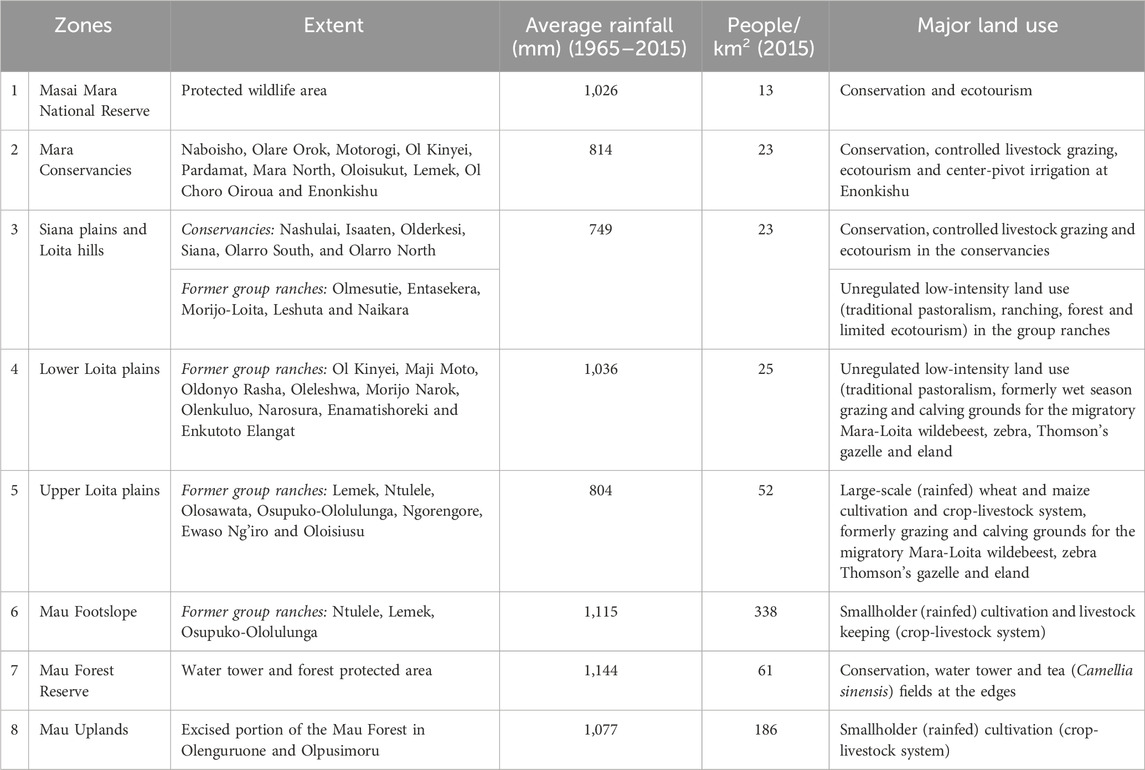
TABLE 1. Characteristics of the eight zones in the Extended Greater Masai Mara Ecosystem (EGMME) showing their extent, average rainfall (mm), human population density and land use.

We relied on our socio-ecological knowledge of the landscape and used the physical boundary for the conservation areas, protection status and land use intensity to subdivide the rangeland into five zones: (i) Masai Mara National Reserve. (ii) Semi-protected wildlife conservancies with controlled livestock grazing alongside wildlife conservation. (iii) Siana plains and Loita hills with low-intensity land use and limited conservation. (iv) Lower Loita plains with low-intensity land use and traditional pastoralism. (v) Upper Loita plains with high-intensity land use and large-scale commercial farms (Table 1). Large-scale (wheat and maize) farming is expanding in the transitional zone at the edge of the low-lying rangeland.

The variation in soil types and seasonality of water availability can introduce additional dissimilarities among cover types in each zone (Chasmer et al., 2020). Three zones were delineated in the highland comprising the Mau Forest Reserve (dense woodland), Mau upland (intensive small-scale rainfed cultivation) and Mau footslope (widespread crop-livestock systems). These areas are wetter and suitable for cultivation. We used a digital elevation model (DEM, SRTM 30 m), human population density and agroecological zonation to separate the zones based on land use intensity. Lastly, we generated 10-km buffers around each zone, which overlapped with the adjacent zone(s), and used them to seamlessly merge the zones to form the EGMME after separately classifying each zone.

2.1.4 Hierarchical classification scheme

A good LULC classification system is typically hierarchically structured to accommodate varying levels of detail ranging from granular to general. It should also be independent of data source and scale (e.g., ground observation, aerial survey or satellite data) (Grunblatt et al., 1989; Jansen and Di Gregorio, 2003). We adopted the Grunblatt et al. (1989) hierarchical vegetation classification system because it meets these criteria and expanded it to incorporate anthropogenic land use (specifically cropland and built-up areas), as well as water bodies, which are not included in the original scheme but represent important cover classes in the study landscape (Table 2). The system (Grunblatt et al., 1989) was developed for heterogeneous cover types using data from ground and aerial surveys to support the long-term monitoring of large-herbivore populations and habitat conditions in the Kenya rangelands (510,726 km²) by the DRSRS and its predecessors (Kenya Rangeland Ecological Monitoring Program (KREMU: 1976–1986) and the Department of Resource Surveys and Remote Sensing (DRSRS:1986–2013)) since 1977 (Ogutu et al., 2016). It is well-tested and standardized for savanna rangelands and relies primarily on structural vegetation heterogeneity and density distribution.

TABLE 2

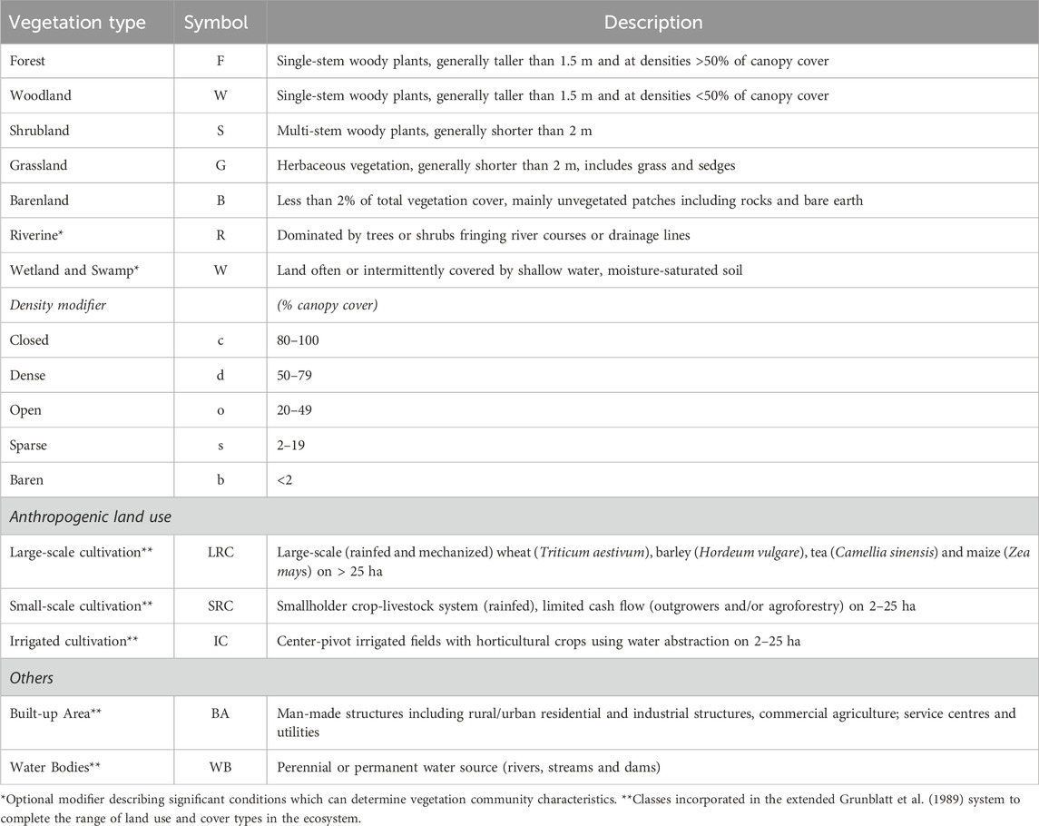
TABLE 2. Summary of the terms and symbols used in the Grunblatt et al. (1989) hierarchical classification scheme and their descriptions.

The scheme has four hierarchical levels for classifying land cover types. The more general category (level 0) only characterizes the primary (lifeform) vegetation cover type (i.e., woodland, shrubland, grassland and barren land), while at level 1, the classes characterize the primary lifeform and canopy cover at a site. Table 2 summarises the terms and symbols used in the classification system. The level 1 classes are defined as dense woodland or Forest (dF), closed Shrubland (cS) or open Grassland, where the cover type (trees, shrubs, and grass) must have >20% canopy cover and preference is given to structural form in the same order. For example, a site with 25% trees, 15% shrubs, 30% grass and 70% bare ground would be called an open Woodland (oW). The sparse modifier is used alongside a class with the greatest canopy cover if there is no form in a higher order with >20% canopy cover and others with >2% (e.g., 0% trees, 2% shrubs, 10% grass, and 90% bare ground would be sparse Grassland (sG).

Level 2 gives a detailed category that describes vegetation community mosaics, where classes are characterized by incorporating the primary (lifeform) vegetation cover and secondary modifiers, and the density modifiers described in the level 1 class. The secondary modifier has terms similar to the primary form (i.e., Wooded or Treed, Shrubbed and Grassed) used as descriptors only when none other than the primary vegetation attains a canopy cover of >20%, and preference is given in the same order. A site with a canopy cover of T25%, S15%, G30% and B70% would be an open Grassed Woodland (oGW), while another site with slightly greater shrub cover (T25%, S22%, G30%, B70%) would be an open Shrubbed Woodland (oSW). The density adjective and secondary modifier describe the primary vegetation cover, with emphasis given to wooded and shrubbed categories, and allowing them to be included if present at >2% and <19% when no other types are present as ‘true’ candidates (or >20%). For example, a site with a canopy of T5%, S15%, G70%, and B30% would be dense ‘Treed’ Grassland (dTG).

The plant heights (tall, low, dwarf) are included at level 3 as modifiers to the primary lifeform, for example, low open Shrubby Grassland. The grazing history and phenological status should be considered when categorizing grass heights. Lastly, level 4 is the most detailed category, which also considers the dominant species in the described vegetation community, for example, Acacia drepanolobium low-Grassed Shrubland. We did not consider levels 3 and 4 in the illustrative example for this study. For example, most of the cropland was either harvested, fallowed or plowed during the dry period except in the wetter uplands, while the herbaceous layer was mostly low, and therefore the plant growth stage (or height) was highly variable.

We incorporated anthropogenic land use at level 2 of the Grunblatt et al. (1989) scheme. The cropland was defined using the landholding (i.e., socio-economic function and field size—a proxy for density), source of water for cultivation (e.g., rainfed or irrigated) and tillage method (e.g., mechanised, tractor or ox-plow) (Meiyappan et al., 2014). Small-scale (2–25 ha) fields are intensive crop-livestock systems with rainfed cultivation and using a tractor or ox-plow for tillage (Longmire and Lugogo, 1989; Meiyappan et al., 2014). The small-scale cultivated areas in the highlands are subdivided into upland and footslope based on relief features. Large-scale (>25 ha) fields are wheat (Triticum aestivum), barley (Hordeum vulgare) and maize (Zea mays) fields under rainfed and mechanized cultivation in the transitional zone at the edge of the rangelands, but large tea (Camellia sinensis) plantations also occur in the upland. The center-pivot irrigated cultivation of horticultural crops is practised through water abstraction at the midstream of the Mara River (Table 1). The built-up area is represented by urban/large rural settlements and other service utilities and the water bodies by the Mara River and its tributaries. Although several other water surfaces also exist such as streams and dams, they are often too small to reliably identify on the medium-resolution image.

2.1.5 Generation of all possible cover classes for the EGMME

We used an a priori classification approach to calculate the number of all possible cover classes based on a combination of vegetation lifeforms and structural attributes including density and canopy cover. Such an approach is used in many fields including soil science and plant taxonomy (e.g., Arnold, 2005; Kusumawardani et al., 2019). Although this approach is effective for producing a standardized classification and consistently describing LULC, it typically requires numerous predefined classes. Further, not all field samples may easily be assigned to one of the predefined classes.

We reviewed the literature and used expert knowledge to construct the set of all possible LULC classes expected in the EGMME. This enabled us to identify all the possible combinations of classification criteria which we used to calculate the number and characterize all the possible expected classes before carrying out the actual field ground-truthing. The classes were defined according to the Grunblatt et al. (1989) classification system using the primary vegetation lifeforms (tree, shrub and grass) and structural attributes including canopy cover or density (e.g., closed, dense, open, sparse and baren) and height (e.g., tall, low, dwarf) to generate 159 possible classes in hierarchical levels 1, 2, and 3.

More precisely, the possible classes are generated as follows. First, we produced codes for all the possible land cover classes in the EGMME using a combination of primary lifeforms: woodland (W), shrubland (S), grassland (G), bare ground (B); density modifiers: dense (d), closed (c), open (o) and sparse (s); and secondary modifiers: wooded (w), shrubbed (s) and grassed (g). Next, we used these to calculate the number of all possible level 1 classes (3 primary lifeforms × 4 density modifiers + 1 barren land = 13) and level 2 classes (3 primary lifeforms × 4 density modifiers × 3 secondary modifiers + 1 barren land = 37). Lastly, we calculated the possible level 3 classes by additionally considering height categories (3 primary lifeforms × 4 density modifiers × 3 secondary modifiers × 3 heights + 1 barren land = 109). This yielded a total of 13 + 37 +109 = 159 classes for levels 1 to 3.

2.1.6 Determining the actual cover classes expected in the EGMME

To determine the actual LULC classes expected in the EGMME, we used information from literature review (e.g., Epp and Agatsiva, 1980; Karime, 1990; Reed et al., 2009), maps from previous studies (Supplementary Table S7), our expert knowledge of the study landscape and experience from DRSRS aerial monitoring surveys on collecting habitat condition data between 1990 and 2015. We identified the detailed structural vegetation cover and cropland classes and compared them with a set of 37 possible expected level 2 classes in the EGMME (Section 2.1.5). A total of 30 natural vegetation cover classes and three anthropogenic land use functions (large- and small-scale rainfed and center-pivot irrigated cultivation) were identified at level 2 of the extended Grunblatt et al. (1989) system. To this, we added two more classes (i.e., built-up areas and water bodies) to yield 35 LULC classes. As a result, 35 classes were actually observed out of the 37 possible level 2 classes expected (Table 4; Figure 8).

2.1.7 Visual image classification and selection of training sites on the images

Image classification was done concurrently with the selection of training sites and involved identifying classes and assigning each training site to one of the expected 35 level 2 classes (Section 2.1.6). We identified a training site and matched the class characteristics inferred from the image with the expected class. Our expert socio-ecological knowledge of the study landscape was crucial in this exercise, besides using a high-resolution Google Earth Pro and 80 oblique photos from aerial sample surveys, some of which fell over the training sites (Section 2.1.1), as aids in the visual image classification (Shrestha and Zinck, 2001). The multispectral image was inspected interactively by inferring the LULC types using image patterns, texture, tone and color (Lillesand et al., 2015). We directly identified the distinct objects on the image based on their patterns that represented familiar features on the ground, for example, large-scale wheat (T. aestivum) fields, tea (C. sinensis) plantations, center-pivot irrigation, built-up areas or large water bodies. Cultivated areas were easily distinguished partly because of their greater internal homogeneity, but the smallholder fields were often harder to discriminate due to a mixture of crops interspersed with small plots of pasture, hedgerows and dwellings.

Prior to selecting the training sites on the image, we partitioned the entire study landscape into eight distinct zones or strata. We then defined a training site as the area of homogeneous 3 × 3 pixels (8,100 m²) containing a single class on the image, digitized the polygon covered by the pixels onto the training layer and assigned it to one of the expected 35-level 2 classes (Section 2.1.6). Some training sites were either irregularly shaped or spanned multiple polygons, especially for rare classes such as riverine gallery forests or ridges, but covered areas comparable in size.

We determined the training sample size for each zone as follows. First, we used stratified random sampling with the eight zones as the strata to select and distribute the training sample sites. Specifically, we used the training sample manager tool in ArcGIS 10.5 to generate 500 random points (UTM coordinates) representing potential training sites on the image for the largest and most heterogeneous zone in the EGMME, the Siana plains and Loita hills zone. Second, we overlaid the DRSRS 5 × 5 km grid cells to guide the systematic search for homogenous pixels around the potential training sample points on the image by zooming on 1 cell at a time, beginning from the bottom-most row and moving upward row by row. We relied on high-resolution Google Earth Pro and oblique aerial photos acquired on some of the grid cells during routine DRSRS aerial surveys (Section 2.1.1) to aid the interpretation of training sites and infer cover classes. The DRSRS grid was also used to spatially relate each potential training site to the corresponding oblique aerial photos for the site and LULC class to the corresponding class determined for the site during the routine DRSRS surveys. This allowed us to identify the LULC class for the 9 contiguous pixels (polygon) containing random points and determine if the pixels qualified for selection as a training site. Third, we identified and excluded all the random points that fell on 3 × 3 pixels with multiple cover classes and were therefore not sufficiently homogenous to assign to a single class. This procedure resulted in 408 of the original 500 random points being selected as training sites for the Siana Plains and Loita Hills zone. Fourth, we estimated the sample size for the entire EGMME using the proportion of the EGMME area (11259.4 km²) to the area of the Siana plains and Loita hills (2704.6 km²) as 408 × (11259.4/2704.6) km² ≅ 1,697. We then distributed the 1,697–408 = 1,289 training samples across the remaining seven zones in proportion to their areas relative to the total area of the EGMME less the area of the Siana plains and Loita hills (Table 3). The sample size for each of the remaining seven zones was therefore calculated as (total area of each zone)/(total area of EGMME -2704.60 = 8554.9) × total number of training sites for the remaining seven zones in the EGMME (1,697–408 = 1,289). The training samples were distributed across the seven zones in a similar way as the Siana Plains and Loita Hills zone. Lastly, we calculated the number of training samples for each class in each zone as (area covered by the class in the zone)/(total area of the zone) × total number of training samples for the zone.

TABLE 3

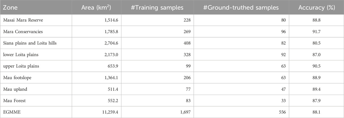
TABLE 3. Summary of the area, number of training samples, number of ground-truthed samples and the degree of agreement between the classes assigned during visual image interpretation and ground truthing for each of the eight zones in the EGMME.

To relate the selected training sites with the Grunblatt et al. (1989) scheme, we created a schema (ESRI, 2016b) in the training sample manager panel in ArcGIS 10.5, then added our expected 35 level 2 classes and assigned each training site with corresponding inferred characteristics to a single class. Next, we digitized a polygon with the random point (UTM coordinate) enclosing the 3 × 3 identical pixels on the training site layer. We ensured that the 9 pixels that form a training sample were indeed homogeneous by using the histogram tool in ArcGIS to compare the frequency distribution of their bands (i.e., the Red, Green and Blue or simply RGB). To ensure the originally generated random points fell on all the expected classes in each zone, we collapsed multiple, visually classified training samples into single, multipart samples to display the total number of samples in a zone and the class distribution. If a class was missed by all the random points (i.e., no random point fell on a pixel containing the class), which was common in small or irregularly shaped areas, particularly for rare classes such as riverine gallery forests or ridges, then two training sites (one for ground-truthing and another for training) were manually added for the missing class.

2.1.8 Selection of ground-truthing samples on the images

We allocated a subset (35%, n = 594) of the 1,697 training sites distributed randomly across the entire 11256 km² EGMME for ground-truthing. We defined the criteria for selecting ground-truthing sites by considering factors that can significantly affect the quality of sampling sites such as road networks and built-up areas. The validation samples were randomly selected from the training sites using buffers (polygons) created along the reference road networks and the peripheries (polygons) of the built-up areas to exclude potential disturbances to the vegetation cover and degraded areas in ArcGIS vers. 10.5 (ESRI, 2016a). We did not create buffers in the cultivated areas where human influence is significant but randomly sampled the accessible areas for ground-truthing sites.

The buffers for selecting ground-truthing samples were designed according to the following criteria. 1) Ground-truthing sites inside the protected areas (Masai Mara National Reserve and Mau Forest Reserve) were randomly selected within a 500 m buffer on both sides of the reference road network because off-road driving and pedestrian movements are restricted except in designated areas. 2) Ground-truthing sites outside the protected areas (Conservancies, Siana plains and Loita hills, and lower Loita plains) were randomly selected within multiple buffers between 200–1,000 m on both sides of the reference road network and 300–1,000 m or more at the periphery of the built-up areas (urban/rural settlements and other major infrastructure). The urban areas are bound to expand towards their peripheries and attract human population and associated activities which typically cause vegetation disturbance and land degradation. 3) No buffer was used in the cultivated areas (upper Loita plains, Mau upland and footslope).

We intersected the buffers and training site layers in ArcGIS vers 10.5 (ESRI, 2016a) to isolate the ground-truthing sites, then systematically and uniquely relabelled the points (UTM-coordinates) and superimposed them onto a topographic map (scale 1:50,000) to help the field team locate each site during the ground-truthing.

2.1.9 Ground-truthing in the field

We actually visited and validated only 556 sites (33%) of the 594 sites (35%) designated for ground-truthing out of the 1,697 training sites. This was because inaccessibility, restrictions on movement and safety concerns made it impossible to visit some sites within the protected areas, while the imminent eviction of local communities from the Mau Forest around the time of our field visits also generated uncertainty and hostility towards our field teams. Consequently, we visited and sampled, for example, only 82 of the 143 sites allocated to the Siana plains and Loita hills, 92 of the 115 sites allocated to the lower Loita plains and 63 of the 72 sites allocated to the Mau footslope zone and relocated 4 sites in the Mau Forest. A few of the visited sites could only be observed from a close range because of the foregoing reasons. To ensure adequate and reliable ground-truthing data were collected during the fieldwork, we replaced the sites that could not be accessed directly with alternative sites about 450 m from the original site that contained similar characteristics (Tables 3 and Supplementary Table S2, S1 Data).

The extended Grunblatt et al. (1989) classification protocol was followed when characterizing and estimating the canopy of vegetation cover and field size of cultivated areas during the ground-truthing in the short (19–29 January; 15–30 February) and long (2–26 July) dry seasons of 2016. The UTM coordinates of the ground-truthing sites were uploaded to a handheld GPS (Trimble^® Juno SB), separately for each zone and supported by toposheets (scale 1:50,000) marked with site geo-locations to locate them in the field.

The field data were collected by two teams trained in remote sensing and ecology and calibrated to minimize observer differences. The teams independently described the structural physiognomy of the dominant and secondary vegetation communities and anthropogenic land use by moving around each site and estimated the percent canopy cover from an elevated platform either by standing on top of a packed vehicle or on a nearby hill. The cropland was classified by field size—a proxy for density, socio-economic function, water source for cultivation and tillage methods. Also recorded were prior disturbance indicators such as livestock grazing, wildlife trampling or destruction, charcoal kilns, deforestation, soil erosion and dominant vegetation species. We did not consider the vegetation growth stage (or height), but this is incorporated at the more detailed level 3 of the hierarchical classification. The vegetation cover and cropland were classified at level 2 of the extended Grunblatt et al. system (Section 2.1.4, Figure 3).

FIGURE 3

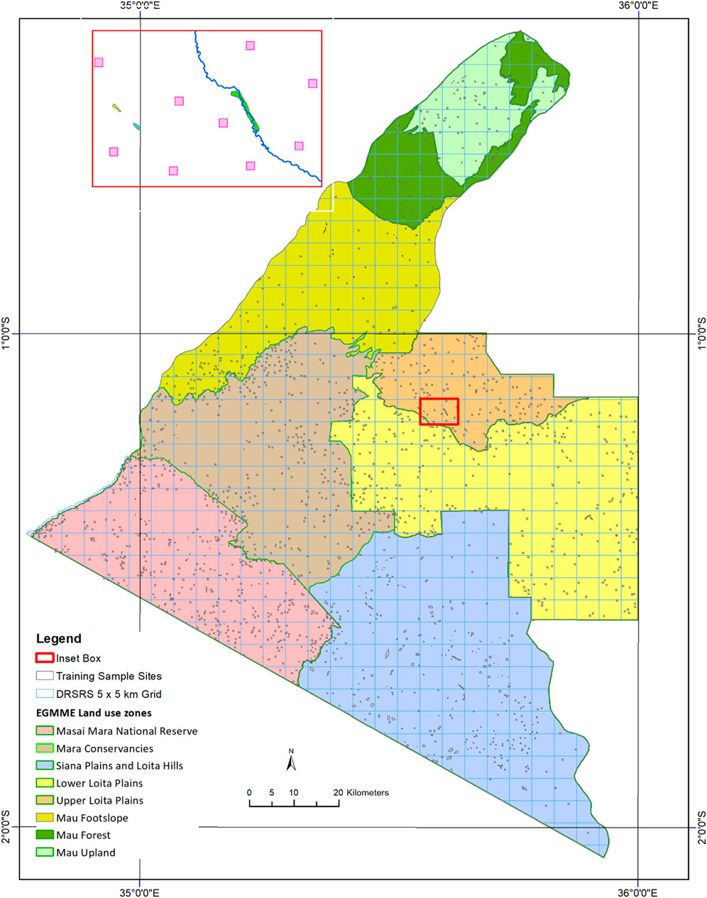
FIGURE 3. Spatial distribution of training sites (black polygons) in the eight zones (coloured background) of the EGMME. The footprint training sites are homogeneous 3 × 3 pixels (90 × 90 m) or irregular shapes in some sites (e.g., riverine gallery forests and ridges on escarpment (Inset box). The DRSRS has used the 5 × 5 km permanent grid shown in the map for aerial monitoring surveys of habitat conditions based on the Grunblatt et al. (1989) system since 1990 (blue lines).

Each sample site measured 3 × 3 pixels or 8,100 m². We subdivided this area into four quadrants each measuring 2025 m² and thoroughly searched each except in the open cultivated areas where an entire site could be observed from one vantage point. We identified the first and the second most dominant vegetation cover types and estimated their percent canopy cover in each quadrant according to the extended Grunblatt et al. classification system and then separately averaged them across all four quadrants making up each site. This average was used to define the common vegetation cover class for the site. The resulting common cover class identified for each site was then standardized by assigning it to the corresponding class that conforms with the Grunblatt classification system. We similarly estimated the field size for cropland and recorded the dominant crop type in each quadrant, then averaged the areas and the common crop type across all four quadrants constituting the site. In addition, we recorded the built-up areas (urban and shopping centres) and types of water bodies (rivers, swamps, dams). Further, we used a hand-held and a compass-guided wooden cross and a site-specific labelled tag to identify geo-tagged horizontal photos taken in each quadrant with a 35 mm camera pointing in each of the four cardinal compass directions (Figure 4). A total of 1,488 such photos were taken in all the 556 sample sites. S2 Data shows the 556 ground-truthed sites in the eight zones, their UTM coordinates, a comparison of the training with the ground-truthed classes, and the respective ground photos taken in each quadrant.

FIGURE 4

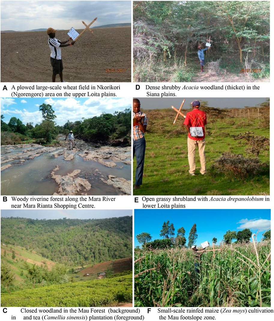
FIGURE 4. Ground-truthing the site-specific LULC data (land cover classes, canopy cover, location tagged label (Loita (zone)-98 (no.)A(quadrat)) and a wooden cross showing the four cardinal compass directions. (A) A plowed large-scale wheat field in Nkorikori (Ngorengore) area on the upper Loita plains. (B) Woody riverine forest along the Mara River near Mara Rianta Shopping Centre. (C) Closed woodland in the Mau Forest (background) and tea (Camellia sinensis) plantation (foreground). (D) Dense shrubby Acacia woodland (thicket) in the Siana plains. (E) Open grassy shrubland with Acacia drepanolobium in lower Loita plains. (F) Small-scale rainfed maize (Zea mays) cultivation in the Mau footslope zone.

2.1.10 Generating the actual training sample dataset for the random forest classifier

We prepared the dataset for training the RF classifier as follows. First, we digitized a polygon layer with the 1,697 training sites. A subset (556 sample sites) of the 1,697 training sites was selected and set aside for ground-truthing (S1 Data). All the training sites (points) were individually labelled and assigned five variables: the UTM coordinates, unique numeric and alphabetic letter codes for the classes and their descriptions.

Second, the information on the training polygons was updated with the actual classes only for those classes that ground-truthing showed to have been misclassified during the image interpretation. However, some new sites were also updated to replace the original sites that could not be validated during the ground-truthing due to the various reasons detailed in Section 2.1.9.

Third, the training polygon layers were overlaid onto the raster image for each zone in the same projection and joined together to link the points (UTM coordinates) for each training site to corresponding pixels with discernible spectral characteristics (S3 Data).

Fourth, the classes for all the ground-truthed sites in each of the eight zones were tallied for their frequency. For example, there were 22 classes in the conservancies zone with unique numeric class codes 4, 6, 7, ..., 43 corresponding to dense grassed shrubland (dGS), open shrubbed grassland (oSG), closed wooded shrubland (cWS) and so on to dense grassland. The frequency for each of the above 22 classes was 12, 24, 6, ..., 1 and for the most common class in this zone was 60. We multiplied the frequency for each class with that for the most common class (multiplier factor = 60) in this zone to ensure an approximately equal probability of randomly selecting any class. The example for the conservancies zone above yielded 720, 1,440, 360, ..., 60 random training samples for the respective classes. Consequently, each zone has its own multiplier factor and the frequency for the most common class over all the eight zones is used as a multiplier factor for the entire ecosystem. The choice of a multiplier factor does not follow any strict rules but larger values (up to the total number of all the pixels for the most common class in a target area or zone) increase the number of randomly selected training samples, which, in turn, improve the classification accuracy (Horning, 2010).

The attributes (UTM coordinates and corresponding classes (response variable)) for the randomly selected training samples above were separately combined with the image band (DN) values (as predictors) for each zone and for the entire EGMME. The number of randomly selected training points and the actual number of sample points may not exactly match because some training sites may not be completely homogeneous and therefore have to be allocated more than one UTM coordinate point. For example, the specified total number of training samples for all the 22 cover classes in the conservancies zone was 16,140 but the number actually selected was 16,280. The final training dataset passed to the RF classifier contained one response variable (numeric class code) and seven predictors (band DN values) (S4 Data).

2.1.11 Implementation, configuration and classification accuracy of the RF classifier

The RF often performs well in classification depending on configurations of its tuning parameters (Kotsiantis, 2010; Belgiu and Drăguţ, 2016). The main tuning parameters for the RF are the number of trees to grow, the number of predictors to consider when splitting a tree node and the minimum number of samples below which a terminal node or tree leaf is not split. We used the RF classifier (Liaw and Wiener, 2002) within the R-script (R Statistical Software, v4.1.1, R Core Team, 2021) of Ned Horning (Text S1; Horning, 2010). We evaluated the performance of this classifier using multiple configurations of the three tuning parameters by executing eight models for each of the eight zones and for the entire EGMME, yielding a total of 72 model runs. The number of trees to grow was set as ntree = 500, 1,000, 2000 and 3,000, the random subsample of predictors (i.e., p = 7 bands) to consider when splitting each tree node was set as mtry = 7/3, therefore either 2 or 3 predictors and the minimum number of samples per tree leaf or terminal node below which no split is attempted (nodesize) was set equal to 1. The RF classifier uses each configuration of ntree, mtry and nodesize to grow trees and assigns each pixel to the most common cover class based on its relative frequency across all the trees. We evaluated the performance of the RF classifier for level 2 classes of the extended Grunblatt et al. classification system but not for the other levels (e.g., the intermediate and general classes) because they are formed by collapsing the secondary and density modifiers of the detailed classes (Table 5).

After the RF classifier has built a prediction tree for the training dataset, the pixels in the rasterized image are used to define an output image block that is passed to the RF classifier for prediction. The RF classifier uses the prediction tree and the predictors (seven image bands) for each point in the output image block to predict the cover class (‘response’) for each point on the output image block. It produces a classified image for all the pixels in the output image block in GeoTIFF format, as well as the following outputs. 1) Class probability image for the classes that received the most votes (pixels with a threshold probability of more than 75%). 2) Classified pixels with inter-class confusion that received the most votes below the 75% threshold. 3) Variable importance plot that provides information on the influence of each predictor variable. 4) Out-of-Bag (OOB) error rate estimate calculated from a cross-tabulation of the error matrix table. 5) Percent error rate given by the number of correct predictions from the OOB sample and computed as 1 minus (sum of correctly classified (diagonal) values divided by the sum of misclassified (column) values) multiplied by 100. 6) Margin (spatial) points (the proportion of votes for the correctly classified samples for a class minus the maximum proportion of votes for the other classes in a zone. The margin (spatial) points can be used to evaluate the data quality. A positive margin value indicates a correctly classified sample and vice versa. The margin points can be superimposed onto the classified image to select classes that need improvement either by removal, relabeling or re-training to enhance data quality. 7) A confusion matrix with statistics for assessing agreement between the predicted classes and the classes in the training dataset by comparing the correctly classified and misclassified classes. The matrix provides the producer’s accuracy which relates to the probability of correctly classifying a sample, the user’s accuracy which measures the probability of the training classes matching the predicted classes and the Kappa coefficient which measures the extent to which the predicted classes compare with the reference classes, where the Kappa values indicate slight (0.1–0.20), fair (0.21–0.40), moderate (0.41–0.60), substantial (0.61–0.80) or perfect (0.81–1.0) agreement (McHugh, 2012). 8) The processing time (computational efficiency) was measured as the difference in minutes between the start and end times of each model run (Figure 7). The models were executed using a 458 GB OS laptop with 16 GB RAM and 11th Gen Intel(R) Core(TM) i5-1135G7 @ 2.40GHz and 2.42 GHz Processor.

Although the RF classifier produced a confusion matrix, we did not use it for evaluating the predictive performance of the classifier and relied instead on the out-of-bag (OOB) error, which is an unbiased estimator of the true error rate (Janitza and Hornung, 2018). Other machine learning classifiers that use bootstrap aggregation such as boosted decision trees also measure prediction accuracy using the OOB error (Friedl et al., 1999; Zhang et al., 2010; Goldstein et al., 2011; Janitza and Hornung, 2018).

2.1.12 Classified LULC map of the EGMME for 2015

We produced the final classified LULC map for the EGMME by merging the individual maps for each zone based on parameter configurations with the highest overall accuracy and computational efficiency ( Figures 5, 7). The final map is the detailed LULC at level 2 of the extended Grunblatt et al. system. The intermediate and general (level 1) classes can be created by aggregating the level 2 classes via dropping the secondary and density modifiers, which demonstrates the hierarchical nature of this approach (S5 Data). We created the final classified map by matching and merging the corresponding features in the 10-km buffer around the eight zones and seamlessly joining them in ERDAS (2008). Then, we used the Clump and Eliminate algorithm to eliminate clusters (salt-and-pepper effect) smaller than the minimum mapping unit (90 × 90 m or 9 pixels) by applying a 3 × 3-pixel majority filter (Lillesand et al., 2015).

FIGURE 5

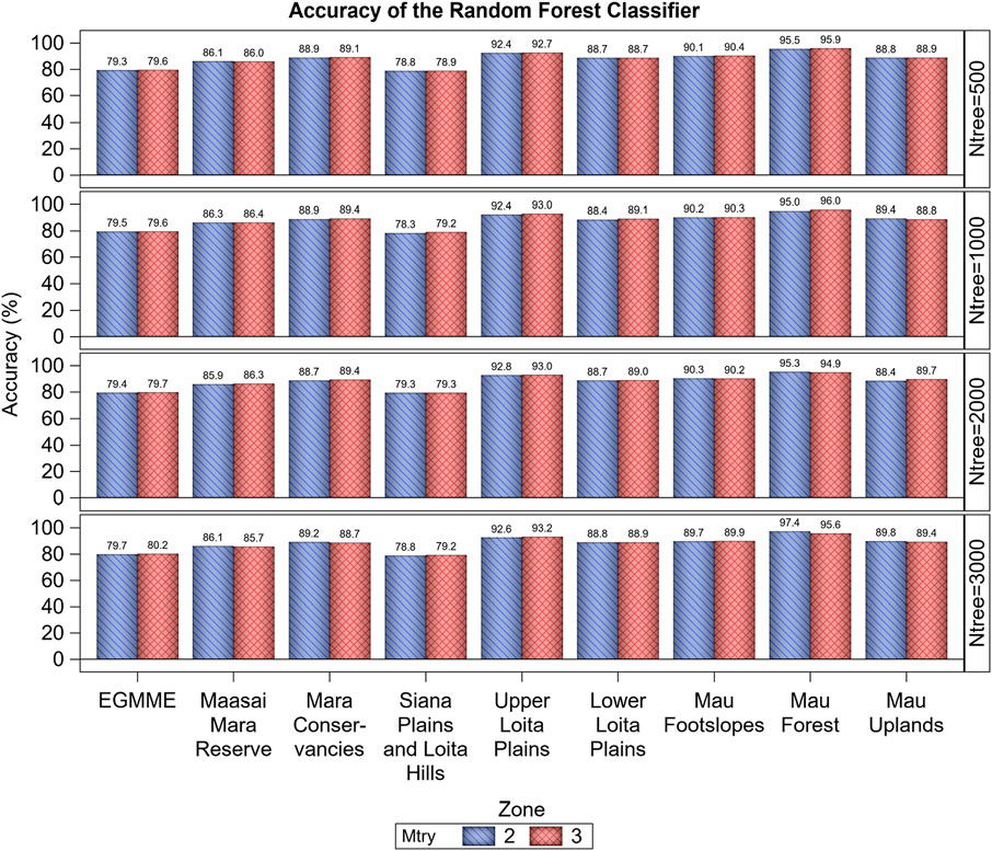
FIGURE 5. Variation in the overall accuracy (%) of the Random Forest classifier based on the Out-of-Bag (OOB) error estimate across the eight zones and the whole study ecosystem (EGMME), the configuration of the number of trees grown (ntree) and the subsample of predictors considered in splitting each tree node (mtry).

3 Results

3.1 Accuracy of visual image classification

We directly compared the classes identified by visual image interpretation with corresponding ground-truthed classes in each of the eight zones to evaluate the interpreter accuracy at 90 × 90 m spatial resolution. This direct measure of accuracy was high and averaged 88.1% (range 80.5%–91.7%) across the zones and increased with land cover homogeneity and intensity of ground-truthing. Consequently, accuracy was the highest for the most intensely ground-truthed conservancies zone (91.7%) and the internally more homogeneous upper Loita plains (90.5%) but the lowest for the internally more heterogeneous Siana plains and Loita hills (80.5%) (Table 3). Accuracy was similarly high and averaged 89.1% (range 50%–100%) across all the classes and increased with increasing internal homogeneity within the classes (Table 4).

TABLE 4

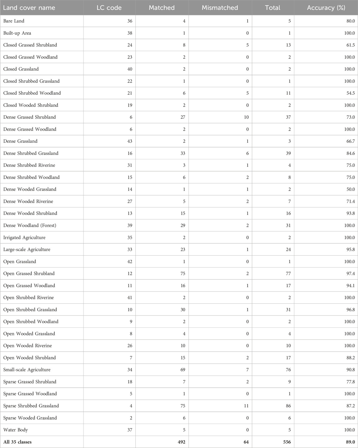
TABLE 4. Summary of the number of times each of the 35 classes assigned during the visual image interpretation matched or did not match the corresponding classes observed during ground-truthing across all the eight zones in the EGMME. LC Code is a unique number assigned to each class.

3.2 Overall and class-specific accuracy of the RF classifier

The accuracy of the RF classifier was higher for the eight zones than for the entire EGMME at 30 × 30 m spatial resolution, highlighting the importance of landscape stratification. Across the eight zones, the overall and class-specific accuracies were higher for the internally more homogeneous zones and classes. Consequently, accuracy was the highest for the more homogeneous Mau Forest (97.4%) and the lowest for the highly heterogeneous Siana plains and Loita hills (79.3%) (Figure 5; Supplementary Tables S4, S5). Accuracy did not vary with increasing number of trees grown, either for each zone or the entire ecosystem, suggesting that using 500 trees would generally yield satisfactory predictions for most practical classification tasks.

The class-specific accuracy varied strikingly among the 35 cover classes, averaging 61.6% and ranging from 25.4%–98.1% (Figure 6; Supplementary Tables S4, S5). This wide variation reflects the underlying high variation in land cover types in this complex landscape. For example, the overall accuracy for the typically more homogeneous dense woody riverine, dense woodland (forest), water bodies and barren land was high, ranging between 93.2% and 98.1%, but that for more heterogeneous dense grassy woodland, open grassy woodland, closed woody shrubland or dense woody shrubland was much lower, ranging between 25.4% and 42.3%. The overall and class-specific accuracy in all the eight zones and in the entire EGMME was little affected by varying the subsample of predictors considered in splitting each tree node (mtry = 2 or 3), suggesting that using 2 or 3 predictors made no material difference to accuracy (Figure 5).

FIGURE 6

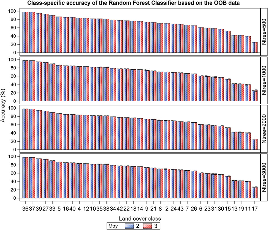
FIGURE 6. Variation in the class-specific accuracy (%) of the Random Forest classifier based on the Out-of-Bag (OOB) data averaged across the 35 LULC classes in the EGMME, the configuration of the number of trees grown (ntree) and the subsample of predictors considered in splitting each tree node (mtry). The x-axis represents the unique numeric code for each class as specified in Table 4 and Supplementary Table S3.

3.3 Computational efficiency of the RF classifier

Computational efficiency of the RF classifier decreased with increasing number of trees grown for all the eight zones except for the internally more heterogeneous Mau Forest and Mau upland (small-scale rainfed cultivation) zones (Figure 7). However, computational efficiency varied only slightly with the subsample of predictors (mtry) considered in splitting each tree node or with the number of classes in a zone. The processing time for the entire ecosystem was much higher than that for all the zones combined, indicating that stratifying the landscape into internally more homogeneous areas enhanced computational efficiency.

FIGURE 7

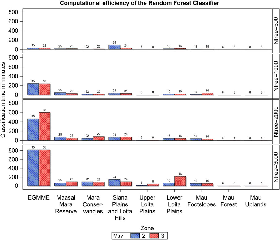
FIGURE 7. Variation in computational efficiency (processing time in minutes) of the Random Forest classifier across the eight zones and the whole ecosystem (EGMME), the configuration of trees grown (ntree) and the subsample of predictors considered in splitting each tree node (mtry). The vertical bar labels are the number of cover classes in each zone.

3.4 Final LULC map of the EGMME, 2015

With the methods outlined above, we produced the first detailed and consistent map of the EGMME at 30 × 30 m spatial resolution for the year 2015, based on land use and structural vegetation heterogeneity and density (Figure 8). We identified a total of 35 detailed LULC classes, which we aggregated into 18 community mosaics and further into five more general classes (Supplementary Tables S3, S6; Supplementary Figures S1, S2). Grassland (35.7%) and shrubland (35.3%) dominated the landscape at the general level of hierarchical classification followed by woodland (12.5%), cropland (16.2%) and other (0.3%). The grassed shrubland (31.9%) and shrubbed grassland (28.9%) were dominant at the intermediate level, but small (13.3%)- and large (2.7%)- scale cultivated areas also occupied sizable areas. At the detailed level 2, the open grassed shrubland (21.8%), followed by sparse shrubbed grassland (10.4%), were the most widespread and occurred largely in the rangelands where the main land use was conservation, traditional pastoralism and ranching (Table 5). The smallholder rainfed cultivation and livestock keeping (crop-livestock system) were prominent in the wetter part of the ecosystem but a few farms were scattered across the rangeland. Large-scale rainfed (wheat and maize) cultivation occurred in the transitional zone with favourable agro-ecological conditions, particularly in the upper Loita plains at the edge of the rangeland, whereas the center-pivot irrigated (horticulture) fields were notable in Enonkishu conservancy within the conservancies zone.

FIGURE 8

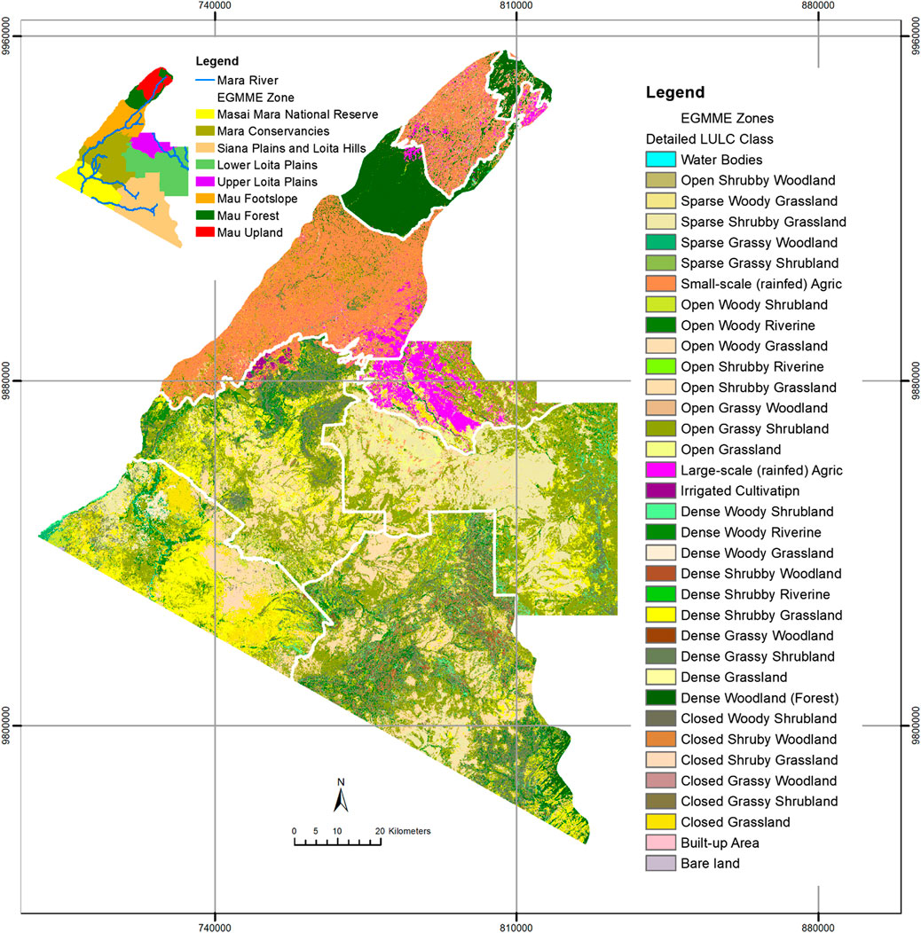
FIGURE 8. A comprehensive LULC map of the EGMME at 30 × 30 m spatial resolution showing the 35 classes of vegetation community mosaics and anthropogenic land use derived from the Landsat 8 image of February 2015. Classification accuracy of 78.8%–95.5% was achieved using ntree = 500 and mtry = 2, separately for each zone (Figure 5). A similar map produced by classifying the whole EGMME without stratification (accuracy = 80.2%) is shown in Supplementary Figure S3.

TABLE 5

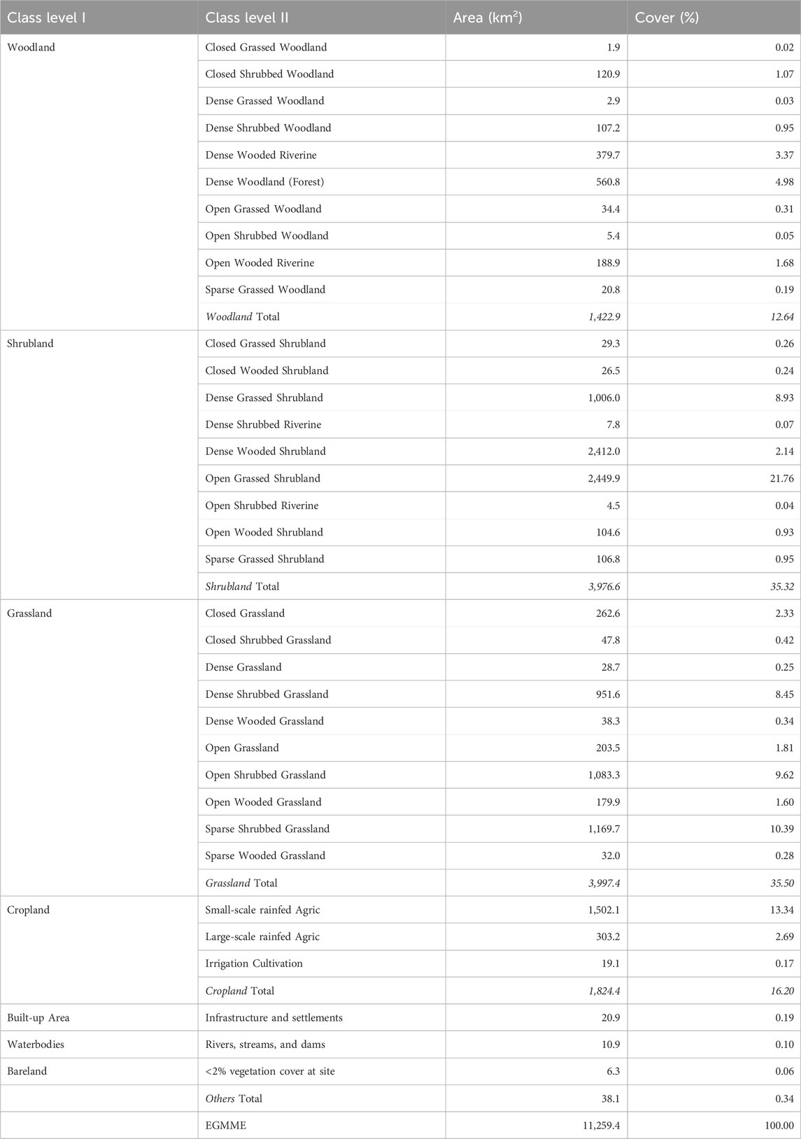
TABLE 5. Summary of the aggregated (general level 1) and detailed (level 2) classes in the Extended Greater Masai Mara Ecosystem (EGMME) (Supplementary Figures S1, S2 and Figure 8).

The most common land cover types in the EGMME are vegetation community mosaics including open grassed shrubland, sparse shrubbed grassland, open shrubbed grassland, dense grassed shrubland, dense shrubbed grassland, dense wooded shrubland and open wooded grassland (Table 5). The riverine shrubbed and wooded gallery forest occurs along the Mara River and its tributaries. A few wetlands are also scattered across the Mara Triangle within the Masai Mara Reserve. The grassland and shrubland are dominant in the Masai Mara Reserve, Mara conservancies, Siana and Loita hills and the Lower Loita plains, whereas woodland occurs in almost equal proportions in the Mara Reserve and the adjacent conservancies but is more widespread in the Mau upland and the Siana plains and Loita hills (Table 6; Figure 8).

TABLE 6

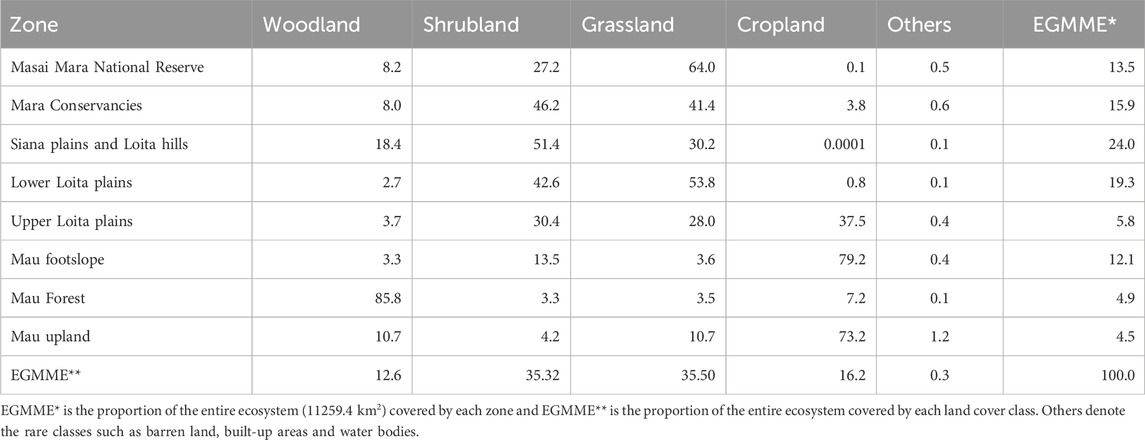
TABLE 6. Summary of the area occupied by the general land cover type in each of the eight zones.

4 Discussion

We developed an approach that blends a hierarchical LULC classification system with the Random Forest classifier, a robust and computationally efficient machine learning algorithm. We also used both landscape stratification and 1,697 training sites distributed according to stratified random sampling and proportionate to the area of each zone. About a third (33%) of the training sites (n = 556) were selected and used for ground-truthing. We evaluate how the accuracy of this approach to LULC classification using medium-resolution remote sensing imagery varies with the following five factors. 1) Landscape stratification to account for landscape heterogeneity. 2) The number and distribution of training and ground-truthing samples. 3) Intra-class heterogeneity. 4) Image resolution, clarity and visual image interpretation. 5) Accuracy and robustness of the classification method. Below, we discuss, in turn, how each of these factors affects accuracy.

4.1 Landscape stratification and LULC accuracy

Stratification enabled the delineation of the study landscape into zones with greater internal homogeneity and smaller variance than the entire study ecosystem, leading to greater classification accuracy. Stratification of the EGMME landscape into eight internally more homogeneous zones also evidently helped minimize the spreading of digital signatures and contamination of adjacent zones during visual image processing. This enhanced accuracy by reducing the likelihood of misclassification. Our approach also reaffirms the importance of stratification in ensuring spatially representative allocation of training and validation sites. As expected, the overall accuracy of the RF classifier was higher for the individual zones, 88.4% (range 79.3%–97.4%) than for the entire ecosystem (80.2%) except in the internally more heterogeneous zones (e.g., Siana plains and Loita hills zone, Masai Mara National Reserve and wildlife conservancies), consistent with findings of other studies (e.g., Smith et al., 2003; Hansen et al., 2013; Sleeter et al., 2013; Cano et al., 2017; Yadav and Congalton, 2018).

Furthermore, landscape stratification improved computational efficiency. Stratification reduced the processing time for the RF classifier such that it was 1.5 times faster for the eight individual zones combined than for the entire EGMME. The gain in computational efficiency with stratification of the RF classifier increased dramatically with decrease in the number of decision trees grown and was four times faster for the individual zones combined than for the entire EGMME for 500 trees but only 0.5–0.8 times faster for 1,000–3,000 trees. Similarly, computational efficiency decreased with increasing number of trees grown for each of the eight zones except for the internally more homogeneous zones, particularly the Mau upland and upper Loita plains that are cultivated areas, and the Mau Forest. Our results, therefore, reinforce the findings of other studies that stratification increases computational efficiency (Loveland and Merchant, 2004; Hansen et al., 2013; Sleeter et al., 2013). However, it has a potential downside that land use transition may be abrupt at the boundaries of the strata (e.g., conservation boundaries), partially reflecting the stratification process itself, rather than ‘true’ land use differences. Our intense ground truthing approach, with samples distributed across strata boundaries, almost certainly minimized this risk.

4.2 Training and ground-truthing sample sizes and LULC accuracy

We used relatively many training (1,697) and validation samples that were well-distributed to achieve a high LULC classification accuracy. Ground-truthing revealed a reasonably high average (88.1%) but substantial variation (80.5%–91.7%) in the accuracy of the visual image classification across the eight zones, corresponding to a misclassification rate of 8.3%–19.5% and showing that internally more heterogeneous zones require relatively more training and validation sites to achieve high accuracy. This has significant implications for the RF classifier because its predictive accuracy, for the subset of the unvalidated training data (1,114 = 1,697 minus 556 training samples), is bounded above by the accuracy of the visual image classification. The ground-truthing showed that although the average class-specific LULC accuracy was high (89.1%), it too varied markedly across the classes (50%–100%) such that the internally more heterogeneous classes exhibited greater misclassification rates and accordingly require relatively more training and ground-truthing samples. It follows logically that even though it can be hard to achieve a large sample size due to inaccessibility, budgetary and time constraints, extensive ground-truthing is essential to achieving accurate LULC classification, especially for complex landscapes such as the EGMME (Congalton, 1991). Other factors that should be considered to improve classification accuracy include suitability, size, shape, distribution, frequency and classes assigned to the training sites (Congalton, 1991; Foody et al., 2006).

4.3 Intra-class heterogeneity and LULC accuracy

Classification accuracy decreased with increasing intra-class heterogeneity for both the visual image and RF classification. The class-specific accuracy ranged between 50% and 100% for the visual image but between 25.4%–98.1% for the RF classifier. Accordingly, the internally more homogeneous classes such as the dense woodland (forest), riverine gallery forest, grassland, large- and small-scale rainfed cultivation, water bodies and barren land had higher accuracies than the more heterogeneous community mosaics. Some rare and therefore less well-represented classes had low classification accuracy as a result.

When classifying detailed structural vegetation heterogeneity and density, it is often difficult to discriminate between classes with different physiognomic characteristics in ecologically similar communities. This is because some classes will emit near-similar spectral reflectances that make them appear indistinguishable on images (Turner and Congalton, 1998). For example, in the EGMME, a recently harvested wheat field and a pasture paddock were hard to distinguish on the medium-resolution image, which complicates their discrimination using spectral responses (Thenkabail, 1999; Reed et al., 2009). Similarly, it is particularly difficult to differentiate classes depicting proximate spectral signatures in communities with overlapping ecological characteristics and thin demarcations such as the shrubbed grassland and grassed shrubland. Other examples of narrowly separable classes in terms of their ecological composition include closed Wooded Grassland (cWG) and densely Wooded Grassland (dWG) as well as dense Shrubbed Grassland (dSG) and closed Shrubbed Grassland (cSG), both of which had the lowest accuracy. However, the estimated inaccuracy is consistent, such that misclassified pixels end up in classes with similar ecological compositions. Also common is the misclassification of functionally distant and disparate classes that are often found together in the same area such as wheat fields, grassland and cultivated pasture, but which appear homogeneous in images. Open and closed grassland often have narrow distinctions but are less likely to be mistaken for open grassed shrubland.

4.4 Image resolution, visual image interpretation and LULC accuracy

The medium-resolution remote sensing images such as Landsat 8 OLI are popular for LULC mapping from local to global scales (Gad and Kusky, 2006; Thi et al., 2019), however, their utility is constrained by limitations inherent in their spatial and temporal resolutions as well as spectral responses, all of which affect visual image interpretation and hence the overall and class-specific accuracies. Because the details of an image are captured by visual inspection, we used well-trained image interpreters with expert knowledge of the study landscape to ensure a dependable identification of the image objects. However, if unreliable or outdated auxiliary data are used to support image interpretation, then this can result in misinterpretation and reduced accuracy. As a result, we relied on high-resolution Google Earth Pro and aerial photos acquired around the same time as the satellite images. These high-resolution images have more pixels and higher-quality information than medium-resolution images. We expect this to enhance the interpreter accuracy, which is the most reliable measure of classification because the classes identified visually on the image are compared with direct field observations. Consequently, any inaccuracy introduced during the visual image inspection can be magnified in the subsequent image processing steps, and reduce the overall accuracy. Moreover, interpreters should be adequately knowledgeable about the study landscape and have sufficient image interpretative skills to minimize misclassification. It is perhaps fair, therefore, to say that it is almost impossible to produce a detailed and accurate LULC map without good socio-ecological knowledge of a landscape.

Our approach refines the Grunblatt et al. (1989) method with respect to spatial resolution. The Grunblatt et al. (1989) method as applied by the DRSRS is typically used to assess the LULC at 5 × 5 km or 5 × 2.5 km spatial resolution from low-flying aircraft (Ogutu et al., 2016). However, we downscaled this to 90 × 90 m (or 3 × 3 homogeneous pixels) during the visual image interpretation and further to 30 × 30 m resolution during the processing of the Landsat 8 OLI image in which the individual pixels form the basis for spectral classification and evaluation of accuracy.

4.5 Integrating the Grunblatt et al. system with the RF classifier

The Grunblatt et al. scheme is a well-tested and standardized classification system that has been used for assessing land use and habitat condition in the Kenya rangelands as part of a long-term monitoring program on trends of large-herbivore populations since 1990 (Ogutu et al., 2016). However, this is the first time this classification system has been blended with the RF classifier for LULC mapping. Besides the RF classifier, the system can also be blended with many other efficient machine-learning or other algorithms used for classification in remote sensing applications. Our approach represents a major improvement over previous LULC classification and mapping in complex social-ecological systems such as African savannas.

4.6 Classified LULC map of the EGMME for 2015

A detailed and accurate map of vegetation heterogeneity and density and land use at the landscape scale is essential but was previously lacking for the EGMME. In order to understand the challenges relating to land cover conversion and modification, and to link habitats to putative drivers of change, a fine and consistent description of the LULC characteristics is required. We have therefore produced granular maps with high overall accuracy based on extensive ground-truthing in the EGMME and a thorough assessment of the classification accuracy. This is the most detailed and consistent classification of the structural vegetation heterogeneity and density for this landscape to date. The maps represent a substantial advance over existing products due to the comparatively many training and ground-truthing samples, efficient classifier and hierarchically consistent and reproducible classification system used. The detailed to general cover classes produced are suitable for reliable multiscalar change detection.

Our approach represents a considerable improvement over the previous mapping efforts in the EGMME landscape, some of which have relied on ad hoc and unreproducible classes or typically assumed rather than assessed classification accuracy (Supplementary Table S7). Some of the earlier maps are generalized and were based on either insufficient ground-truthing data or used non-robust classifiers or inefficient analytical tools, and therefore differ markedly even for the same study area. For example, Epp and Agatsiva (1980) identified 46 cover classes and grouped them into 12 general categories in the GMME (7,500 km²) using data from multiple sources (ground, aerial and satellite images) acquired between 1973 and 1976. They relied on the modified Pratt et al. (1966) system to classify the physiognomic characteristics of the vegetation, particularly height and canopy cover. Broten and Said (1995) later re-grouped the Epp and Agatsiva (1980) cover classes into 9 classes and augmented these with 8 more classes from Msafiri (1984) to yield 17 more general cover types. They estimated the most extensive vegetation cover in the ecosystem as shrubland (45%), dwarf shrubland (21%) and grassland (26%). Reed et al. (2009) used Land ETM + images and a fuzzy classification and post-classification fuzzy convolution and 859 ground-truthing samples. They applied the original Grunblatt et al. (1989) scheme only to display their 40 land cover classes, which excluded the anthropogenic land use, across 24000 km² of the 40000 km² Greater Serengeti-Mara Ecosystem (GSME) that lies largely in Tanzania, with a small portion overlapping our study landscape in Kenya. Reed et al. (2009) stratified the GSME into three zones and classified each separately but did not consider classifying the entire ecosystem as a single entity. They did ground truthing using multiple methods, none of which estimated the structural vegetation heterogeneity and density according to the Grunblatt et al. (1989) method. The FAO-Africover Kenya mapped the entire EGMME landscape as part of a Kenya-wide mapping project involving visual interpretation of Landsat ETM images acquired in 2000. They used the FAO/UNEP Land Cover Classification System (LCCS), relying mainly on a dichotomous and modular hierarchy, limited fieldwork and broad classes (Ahlqvist, 2008). The World Resources Institute (WRI)/FAO/DRSRS (2008) updated the FAO-Africover Kenya map using the FAO/GLCN methods. More recent LULC mapping efforts in the EGMME and the rest of Narok County have used various ad hoc classification systems and so have produced contrasting and often inconsistent and unreproducible LULC classes (Supplementary Table S7).

4.7 Further refinements and extensions of the Grunblatt et al-RF classifier

We have extended the Grunblatt et al. (1989) system to incorporate anthropogenic land use, a feature not considered in the original scheme (Section 2.1.4) and downscaled its coverage to finer spatial resolutions. The approach can also readily be extended to include LULC classes specific to particular study areas. We chose the Grunblatt et al. (1989) system because it uses systematic criteria, a complete set of diagnostic elements and precise and unambiguous class definitions to achieve consistent, hierarchical and reproducible classification. The scheme can be used to consistently classify LULC at the landscape through regional and continental to global scales.

Improving the accuracy of the Grunblatt et al-RF classifier, as with all LULC classification systems, can be challenging and revolves around the determination of appropriate number of classes to be used because too many or too few of these classes are likely to poorly represent the actual classes in a study landscape. For the Grunblatt et al. method, the maximum number of classes is bounded above by the expected possible classes, which can be determined prior to ground-truthing. Also, the accuracy of the Grunblatt et al.-RF classifier can be enhanced by using a very high resolution (VHR) image for mapping highly heterogeneous landscapes and complex socio-ecological systems such as savannas. However, at least two challenges are likely to arise when using such images for LULC mapping. (i) The cost of images and time spent on analysis can become prohibitive; however, as image processing technology advances and image cost reduces, we expect these to become less in future. (ii) The image pixel size may be smaller than the coverage of target objects such as tree canopy. This is a fundamental challenge and perhaps the most important concern in improving the accuracy of our approach. For example, using images such as the WorldView-1 and GeoEye-1 with a 0.5 m spatial resolution may result in a tree canopy covering several adjacent pixels, which would require a more complex object-oriented analysis instead of the ‘traditional’ pixel-based classification (Whiteside and Ahmad, 2005).

The Grunblatt et al. (1989) scheme is best applied to medium (e.g., Landsat 8 OLI) and higher resolution images with pixels that cover entire target objects such as tree canopies at the landscape scale, but its scale-independent classes permit the description of objects and areas smaller than a pixel in size. At finer spatial resolutions, this scheme can be used together with robust classifiers such as the RF to provide even more granular classes and higher accuracy. Moreover, the increasing temporal frequency of satellite images with fine spatial resolution opens up new frontiers for using this approach to reliably and efficiently monitor fine-resolution LULC changes in space and time (Brown et al., 2022). We anticipate further improvements in the accuracy and computational efficiency of this approach as more efficient analytical tools, machine learning classifiers and platforms that provide multi-dimensional (open access) datasets become more widely available and affordable.

5 Conclusion

We have developed an approach to LULC classification that blends the hierarchical Grunblatt et al. (1989) classification scheme with the robust random forest classifier. The approach is very flexible and general and can be used at landscape to global scales, with stratified classification as an important method to cope with large-scale landscape heterogeneity. It is especially suitable for ecosystems with relatively fuzzy differences between LULC categories, such as savannas. Our extensive ground-truthing data can be used to improve wider mapping efforts at regional, continental and global scales. We have used large training (1,697) and ground-truthing (556) samples to assess the accuracy of the method in a relatively vast and complex socio-ecological system, the Extended Greater Masai Mara Ecosystem in Kenya. We anticipate the accuracy and computational efficiency of the approach to increase as more efficient classification algorithms and high-resolution data to aid image interpretation become more widely available.

Our application of the approach supports the following general conclusions. The Grunblatt et al.-RF classifier can accurately predict detailed land use and structural vegetation heterogeneity and density and land use even for vast and complex landscapes. The predictive accuracy and computational efficiency of the approach are both enhanced by landscape stratification. Using internally more homogeneous zones with the RF classifier increases accuracy and computational efficiency, both of which reduce with increasing landscape area and complexity. Similarly, accuracy increases with increasing intra-class homogeneity. Using more training and validation samples improves the accuracy of the LULC classification approach.

Growing 500 trees for the RF classifier yields sufficient accuracy for most practical classification tasks at relatively low computational cost. The size of subsamples of predictor variables considered when splitting a tree node using relatively few predictors (seven image bands in our case) has a negligible effect on the predictive accuracy and computational efficiency of the RF classifier. We have produced a granular and reliable map of the EGMME with consistent and reproducible LULC classes, and shown how to collapse the detailed classes into intermediate and more general categories. The generalized classes may be more suitable for general change detection than the more detailed classes, but the latter are more appropriate when a consistent classification system is desired. The digital maps and photos acquired during the ground truthing are provided as aids for wider ground-truthing efforts at regional to global scales.

Data availability statement

The original contributions presented in the study are included in the article/Supplementary Material, further inquiries can be directed to the corresponding author.

Ethics statement

No human studies are presented in the manuscript. Written informed consent was obtained from the individual(s) for the publication of any potentially identifiable images or data included in this article.

Author contributions

GO, HO, and MS conceived the study; GO, MO, and SK conducted ground-truthing in the field; GO, JO, and MO analyzed the data; GO prepared the initial draft. All authors contributed to the article and approved the submitted version.

Funding

This project has received funding from the European Union’s Horizon 2020 research and innovation programme under Grant Agreement No. 641918 through the AfricanBioServices project. JO was additionally supported by a grant from the German Research Foundation (DFG, Grant # 257734638). RB considers this work a contribution to RAMONA under ESA contract No. 4000136180/21/I-NB. This research was carried out as part of the PhD thesis of GO within the EU-funded AfricanBioServices Project.

Acknowledgments

GO thanks Dr Patrick W. Wargute, Director of the Directorate of Resource Surveys and Remote Sensing of Kenya (DRSRS) for permission to do this study, and DRSRS and RUG for institutional support. We are grateful to Prof. Eivin Røskaft (NTNU) for support within the AfricanBioservices project and Prof. Jess Grunblatt for useful suggestions on the classification system. We are also grateful to Rehema Boke, Peter Solonka, Robert Kimtai, and Steven Montet for their help with fieldwork. We thank the Narok County Government (NCG), senior wardens Samson Lenjir (Masai Mara National Reserve) and James Kintai (Mara Triangle Conservancy), and conservancy managers for permission to conduct fieldwork and to local landowners for permission to access their private properties for fieldwork.

Conflict of interest

The authors declare that the research was conducted in the absence of any commercial or financial relationships that could be construed as a potential conflict of interest.

Publisher’s note

All claims expressed in this article are solely those of the authors and do not necessarily represent those of their affiliated organizations, or those of the publisher, the editors and the reviewers. Any product that may be evaluated in this article, or claim that may be made by its manufacturer, is not guaranteed or endorsed by the publisher.

Supplementary material

The Supplementary Material for this article can be found online at: https://www.frontiersin.org/articles/10.3389/frsen.2023.1188635/full#supplementary-material

References

Ahlqvist, O. (2008). In search of classification that supports the dynamics of science: the FAO land cover classification system and proposed modifications. Environ. Plan. B Plan. Des. 35, 169–186. doi:10.1068/b3344

CrossRef Full Text | Google Scholar

Amro, I., Mateos, J., Vega, M., Molina, R., and Katsaggelos, A. K. (2011). A survey of classical methods and new trends in pansharpening of multispectral images. EURASIP J. Adv. Signal Process. 2011, 79–22. doi:10.1186/1687-6180-2011-79

CrossRef Full Text | Google Scholar

Amuyunzu, C. L. (1984). Land resources inventory as a basis of land evaluation and rural development: the role of remote sensing techniques. M.Sc. thesis. Netherlands: ITC.

Google Scholar

Anderson, J. R., Hardy, E. E., Roach, J. T., and Witmer, R. E. (1976). A land use and land cover classification system for use with remote sensor data. Washington, DC: U.S. Government Printing Office, Geological Survey Professional Paper No. 964, 28.

Google Scholar

Arnold, R. W. (2005). “Classification of soils. Pages 204–210,” in Encyclopedia of soils in the environment. Editor D. Hillel (Oxford: Elsevier).

Google Scholar

Ayuyo, I. O. (2021). Impact of land cover, land use and climate change on the hydrological regimes of the Mara River Basin. PhD Thesis. Nairobi, Kenya: University of Nairobi. Available at: http://erepository.uonbi.ac.ke/handle/11295/157098.

Google Scholar

Bajocco, S., Angelis, A., Perini, L., Ferrara, A., and Salvati, L. (2012). The impact of land use/land cover changes on land degradation dynamics: a mediterranean case study. Environ. Manag. 49, 980–989. doi:10.1007/s00267-012-9831-8

PubMed Abstract | CrossRef Full Text | Google Scholar

Bartzke, G. S., Ogutu, J. O., Mukhopadhyay, S., Mtui, D., Dublin, H. T., and Piepho, H.-P. (2018). Rainfall trends and variation in the Maasai Mara ecosystem and their implications for animal population and biodiversity dynamics. PloS one 13, e0202814. doi:10.1371/journal.pone.0202814

PubMed Abstract | CrossRef Full Text | Google Scholar

Bedelian, C., and Ogutu, J. O. (2017). Trade-offs for climate-resilient pastoral livelihoods in wildlife conservancies in the Mara ecosystem, Kenya. Pastoralism 7, 10. doi:10.1186/s13570-017-0085-1

PubMed Abstract | CrossRef Full Text | Google Scholar

Belgiu, M., and Drăguţ, L. (2016). Random forest in remote sensing: a review of applications and future directions. ISPRS J. Photogrammetry Remote Sens. 114, 24–31. doi:10.1016/j.isprsjprs.2016.01.011

CrossRef Full Text | Google Scholar

Berhane, T. M., Lane, C. R., Wu, Q., Autrey, B. C., Anenkhonov, O. A., Chepinoga, V. V., et al. (2018). Decision-tree, rule-based, and random forest classification of high-resolution multispectral imagery for wetland mapping and inventory. Remote Sens. 10, 580. doi:10.3390/rs10040580

PubMed Abstract | CrossRef Full Text | Google Scholar

Betts, F. (1953). Report on the forest areas of Narok. Kenya archives document DC/NRK 3.

Google Scholar

Bhola, N., Ogutu, J. O., Piepho, H.-P., Said, M. Y., Reid, R. S., Hobbs, N. T., et al. (2012). Comparative changes in density and demography of large herbivores in the Masai Mara Reserve and its surrounding human-dominated pastoral ranches in Kenya. Biodivers. Conservation 21, 1509–1530. doi:10.1007/s10531-012-0261-y

CrossRef Full Text | Google Scholar

Binaghi, E., Brivio, P. A., Ghezzi, P., and Rampini, A. (1999). A fuzzy set-based accuracy assessment of soft classification. Pattern Recognit. Lett. 20, 935–948. doi:10.1016/s0167-8655(99)00061-6

CrossRef Full Text | Google Scholar

Braun-Blanquet, J. (1932). Plant sociology. New York: McGraw-Hill Book Company.

Google Scholar

Breiman, L. (2001). Random forests. Mach. Learn. 45, 5–32. doi:10.1023/a:1010933404324

CrossRef Full Text | Google Scholar

Broten, M. D., and Said, M. (1995). “Population trends of ungulates in and around Kenya’s Masai Mara Reserve,” in Serengeti II: Dynamics, Management and Conservation of an Ecosystem. Editors A. R. E. Sinclair, and P. Arcese (Chicago: University of Chicago Press), 169–193.

Google Scholar

Brown, C. F., Brumby, S. P., Guzder-Williams, B., Birch, T., Hyde, S. B., Mazzariello, J., et al. (2022). Dynamic World, Near real-time global 10 m land use land cover mapping. Sci. Data 9, 251. doi:10.1038/s41597-022-01307-4

CrossRef Full Text | Google Scholar

Bylander, T. (2002). Estimating generalization error on two-class datasets using out-of-bag estimates. Mach. Learn. 48, 287–297. doi:10.1023/a:1013964023376

CrossRef Full Text | Google Scholar

Cano, E., Denux, J.-P., Bisquert, M., Hubert-Moy, L., and Chéret, V. (2017). Improved forest-cover mapping based on MODIS time series and landscape stratification. Int. J. Remote Sens. 38, 1865–1888. doi:10.1080/01431161.2017.1280635

CrossRef Full Text | Google Scholar

Cavalin, P., and Oliveira, L. S. (2017). “A review of texture classification methods and databases,” in 2017 30th SIBGRAPI Conference on graphics, patterns and images tutorials (SIBGRAPI-T), Niteroi, Brazil, 17-18 October 2017 (IEEE).

CrossRef Full Text | Google Scholar

Chasmer, L., Mahoney, C., Millard, K., Nelson, K., Peters, D., Merchant, M., et al. (2020). Remote sensing of boreal wetlands 2: methods for evaluating boreal wetland ecosystem state and drivers of change. Remote Sens. 12, 1321. doi:10.3390/rs12081321

CrossRef Full Text | Google Scholar

Chavez, J. (1996). Image-based atmospheric corrections - revisited and improved. Photogrammetric Eng. Remote Sens. 62, 1025–1036.

Google Scholar

Clover, P. E., and Trump, E. C. (1970). An ecological survey of the Narok district of Kenya, masailand Part II vegetation. Nairobi, Kenya: Food and Agricultural Organization of the United Nations FAO. Available at: https://edepot.wur.nl/485413.

Google Scholar

Congalton, R. G. (1991). A review of assessing the accuracy of classifications of remotely sensed data. Remote Sens. Environ. 37, 35–46. doi:10.1016/0034-4257(91)90048-b

CrossRef Full Text | Google Scholar

Coppin, P. R., and Bauer, M. E. (1996). Digital change detection in forest ecosystems with remote sensing imagery. Remote Sens. Rev. 13 (3-4), 207–234. doi:10.1080/02757259609532305

CrossRef Full Text | Google Scholar

DiGregorio, A., and Jansen, L. J. M. (2000). Land cover classification system, concepts and user manual. GCP/RAF/287/ITA Africover. Rome: Food and Agriculture Organization of the United Nations Publishing Service.

Google Scholar

Dublin, H. T. (1986). Decline of the Mara woodlands: the role of fire and elephants. PhD Thesis. Columbia: University of British Columbia.

Google Scholar

Dublin, H. T. (1991). Dynamics of the serengeti-mara woodlands: an historical perspective. For. Conservation Hist. 35, 169–178. doi:10.2307/3983496

CrossRef Full Text | Google Scholar

Dublin, H. T. (1995). “Vegetation dynamics in the serengeti-mara ecosystem: the role of elephants, fire, and other factors,” in Serengeti II Dynamics, Management, and Conservation of an Ecosystem. Editors A. R. E. Sinclair, and P. Arcese, 71.

Google Scholar

Ekstrand, S. (1996). Landsat TM-based forest damage assessment: correction for topographic effects. Photogrammetric Eng. Remote Sens. 62, 151–162.

Google Scholar

Epp, H., and Agatsiva, J. (1980). Habitat types of the mara-narok area, western Kenya. Nairobi, Kenya: KREMU, Ministry of Finance and Planning.

Google Scholar

ESRI (2016a). ArcMap desktop: release 10.5. Redlands, CA: Environmental Systems Research Institute.

Google Scholar

ESRI (2016b). Training sample manager. Available at: https://pro.arcgis.com/en/pro-app/latest/help/analysis/image-analyst/training-samples-manager.html.

Google Scholar

Foody, G., Mathur, A., Sanchez Hernandez, C., and Boyd, D. (2006). Training set size requirements for the classification of a specific class. Remote Sens. Environ. 104, 1–14. doi:10.1016/j.rse.2006.03.004

CrossRef Full Text | Google Scholar

Franklin, S. E., and Giles, P. T. (1995). Radiometric processing of aerial and satellite remote-sensing imagery. Comput. Geosciences 21, 413–423. doi:10.1016/0098-3004(94)00085-9

CrossRef Full Text | Google Scholar

Friedl, M. A., Brodley, C. E., and Strahler, A. H. (1999). Maximizing land cover classification accuracies produced by decision trees at continental to global scales. IEEE Trans. Geoscience Remote Sens. 37, 969–977. doi:10.1109/36.752215

CrossRef Full Text | Google Scholar

Gad, S., and Kusky, T. (2006). Lithological mapping in the Eastern Desert of Egypt, the Barramiya area, using Landsat thematic mapper (TM). J. Afr. Earth Sci. 44, 196–202. doi:10.1016/j.jafrearsci.2005.10.014

CrossRef Full Text | Google Scholar

Ghimire, B., Rogan, J., Galiano, V. R., Panday, P., and Neeti, N. (2012). An evaluation of bagging, boosting, and random forests for land-cover classification in cape cod, Massachusetts, USA. GIScience Remote Sens. 49, 623–643. doi:10.2747/1548-1603.49.5.623

CrossRef Full Text | Google Scholar

Gilabert, M. A., Conese, C., and Maselli, F. (1994). An atmospheric correction method for the automatic retrieval of surface reflectances from TM images. Int. J. Remote Sens. 15, 2065–2086. doi:10.1080/01431169408954228

CrossRef Full Text | Google Scholar

Giles, P. T. (2001). Remote sensing and cast shadows in mountainous terrain. Photogrammetric Eng. Remote Sens. 67, 833–839.

Google Scholar

Gislason, P. O., Benediktsson, J. A., and Sveinsson, J. R. (2006). Random Forests for land cover classification. Pattern Recognit. Remote Sens. 27, 294–300. doi:10.1016/j.patrec.2005.08.011

CrossRef Full Text | Google Scholar

Glover, P. E., and Trump, E. C. (1970). “An ecological survey of the Narok District of Kenya Masailand,” in The vegetation. 2nd Edn. Kenya National Parks Report. Nairobi, 157.

Google Scholar

Goldstein, B. A., Polley, E. C., and Briggs, F. B. S. (2011). Random forests for genetic association studies. Stat. Appl. Genet. Mol. Biol. 10, 32. doi:10.2202/1544-6115.1691

PubMed Abstract | CrossRef Full Text | Google Scholar

Grunblatt, J., Ottichilo, W. K., and Sinange, R. K. (1989). A hierarchical approach to vegetation classification in Kenya. Afr. J. Ecol. 27, 45–51. doi:10.1111/j.1365-2028.1989.tb00927.x

CrossRef Full Text | Google Scholar

Hansen, J., Sato, M., Ruedy, R., Lacis, A., and Oinas, V. (2000). Global warming in the twenty-first century: an alternative scenario. Proc. Natl. Acad. Sci. 97, 9875–9880. doi:10.1073/pnas.170278997

PubMed Abstract | CrossRef Full Text | Google Scholar

Hansen, M. C., Potapov, P. V., Moore, R., Hancher, M., Turubanova, S. A., Tyukavina, A., et al. (2013). High-resolution global maps of 21st-century forest cover change. Science 342, 850–853. doi:10.1126/science.1244693

PubMed Abstract | CrossRef Full Text | Google Scholar

Homewood, K., Chenevix Trench, P., and Brockington, D. (2012). Biodiversity conservation and poverty alleviation: exploring the evidence for a link. John Wiley & Sons.

Google Scholar

Horning, N. 2010. Random Forests: an algorithm for image classification and generation of continuous fields data sets.

Google Scholar

Hussain, M., Chen, D., Cheng, A., Wei, H., and Stanley, D. (2013). Change detection from remotely sensed images: from pixel-based to object-based approaches. ISPRS J. photogrammetry remote Sens. 80, 91–106. doi:10.1016/j.isprsjprs.2013.03.006

CrossRef Full Text | Google Scholar

IPBES (2018). “The IPBES assessment report on land degradation and restoration,” in Secretariat of the intergovernmental science-policy platform on biodiversity and ecosystem services. Editors L. Montanarella, R. Scholes, and A. Brainich (Bonn, Germany: IPBES), 744. doi:10.5281/zenodo.3237392

CrossRef Full Text | Google Scholar

IPBES (2019). “Global assessment report on biodiversity and ecosystem services of the intergovernmental science-policy platform on biodiversity and ecosystem services,” in IPBES secretariat. Editors E. S. Brondizio, J. Settele, S. Díaz, and H. T. Ngo (Bonn, Germany: IPBES), 1148. doi:10.5281/zenodo.3831673

CrossRef Full Text | Google Scholar

Janitza, S., and Hornung, R. (2018). On the overestimation of random forest’s out-of-bag error. PLOS ONE 13, e0201904. doi:10.1371/journal.pone.0201904

PubMed Abstract | CrossRef Full Text | Google Scholar

Jansen, L., and Di Gregorio, A. (2003). Land-use data collection using the “land cover classification system”: results from a case study in Kenya. Land Use Policy 20, 131–148. doi:10.1016/s0264-8377(02)00081-9

CrossRef Full Text | Google Scholar

Jung, M., Koirala, S., Weber, U., Ichii, K., Gans, F., Camps-Valls, G., et al. (2019). The FLUXCOM ensemble of global land-atmosphere energy fluxes. Sci. Data 6, 74. doi:10.1038/s41597-019-0076-8

PubMed Abstract | CrossRef Full Text | Google Scholar

Karime, O. N. I. (1990). The changing land use patterns in the ngorengore/loita plains technical report No. 135. Nairobi, Kenya: Department of Resource Surveys & Remote Sensing DRSRS.

Google Scholar

Keshava, N., and Mustard, J. F. (2002). Spectral unmixing. IEEE signal Process. Mag. 19, 44–57. doi:10.1109/79.974727

CrossRef Full Text | Google Scholar

Kija, H., Ogutu, J. O., Mangewa, L., Bukombe, J., Verones, F., Graae, B., et al. (2020). Land use and land cover change within and around the greater Serengeti ecosystem, Tanzania. Am. J. Remote Sens. 8, 1–19. doi:10.11648/j.ajrs.20200801.11

CrossRef Full Text | Google Scholar

Kimanzi, J. K., and Wishitemi, B. E. L. (2001). Effects of land use changes on herbivores of masai mara ecosystem. Int. J. Environ. Stud. 58, 727–740. doi:10.1080/00207230108711364

CrossRef Full Text | Google Scholar

Kotsiantis, S. B. (2010). Combining bagging, boosting, rotation forest and random subspace methods. Artif. Intell. Rev. 35, 223–240. doi:10.1007/s10462-010-9192-8

CrossRef Full Text | Google Scholar

Krig, S. (2014). “Ground truth data, content, metrics, and analysis,” in Computer vision metrics: survey, taxonomy, and analysis. Editor S. Krig (Berkeley, CA: Apress), 283–311.

CrossRef Full Text | Google Scholar

Kuchar, P. (1979). A methodology for sampling vegetation in order to monitor condition, trend and plant biomass in Kenya rangeland. Nairobi: Ministry of Planning and National Development, Department of Resource Surveys and Remote Sensing.

Google Scholar

Kusumawardani, W., Muzzazinah, S., and Ramli, M. (2019). Plant taxonomy learning and research: a systematics review. AIP Conf. Proc. 2194, 020051. doi:10.1063/1.5139783

CrossRef Full Text | Google Scholar

Lambin, E., Geist, H., and Lepers, E. (2003). Dynamics of Land-use and land-cover change in tropical regions. Annu. Rev. Environ. Resour. 20, 49205–49241. doi:10.1146/annurev.energy.28.050302.105459

CrossRef Full Text | Google Scholar

Lamprey, R. H. (1984). Masai impact on Kenya savanna vegetation: a remote sensing approach. PhD Thesis. Aston: Aston University.

Google Scholar

Lamprey, R. H., and Reid, R. S. (2004). Expansion of human settlement in Kenya’s Maasai Mara: what future for pastoralism and wildlife? J. Biogeogr. 31, 997–1032. doi:10.1111/j.1365-2699.2004.01062.x

CrossRef Full Text | Google Scholar

Li, W., Buitenwerf, R., Munk, M., Amoke, I., Bøcher, P. K., and Svenning, J.-C. (2020a). Accelerating savanna degradation threatens the Maasai Mara socio-ecological system. Glob. Environ. Change 60, 102030. doi:10.1016/j.gloenvcha.2019.102030

CrossRef Full Text | Google Scholar

Li, W., Buitenwerf, R., Munk, M., Bøcher, P. K., and Svenning, J.-C. (2020b). Deep-learning based high-resolution mapping shows woody vegetation densification in greater Maasai Mara ecosystem. Remote Sens. Environ. 247, 111953. doi:10.1016/j.rse.2020.111953

CrossRef Full Text | Google Scholar

Liaw, A., and Wiener, M. (2002). Classification and regression by randomForest. R. news 2, 18–22.

Google Scholar

Lillesand, T., Kiefer, R. W., and Chipman, J. (2015). Remote sensing and image interpretation. John Wiley & Sons.

Google Scholar

Lillesand, T. M., and Kiefer, R. W. (1987). Remote sensing and image interpretation. Second edition. Wiley.

Google Scholar

Longmire, J. L., and Lugogo, J. (1989). “The economics of small-scale wheat production technologies for Kenya,” in CIMMYT economics working paper 89/01 (Mexico: CIMMYT), 65. Avalliable at: https://repository.cimmyt.org/handle/10883/833.

Google Scholar

Loveland, T. R., and Merchant, J. M. (2004). Ecoregions and ecoregionalization: geographical and ecological perspectives. Environ. Manag. 34, S1–S13. doi:10.1007/s00267-003-5181-x

PubMed Abstract | CrossRef Full Text | Google Scholar

Loveland, T. R., Reed, B. C., Brown, J. F., Ohlen, D. O., Zhu, Z., Yang, L., et al. (2000). Development of a global land cover characteristics database and IGBP DISCover from 1 km AVHRR data. Int. J. Remote Sens. 21, 1303–1330. doi:10.1080/014311600210191

CrossRef Full Text | Google Scholar

Løvschal, M., Håkonsson, D. D., and Amoke, I. (2019). Are goats the new elephants in the room? Changing land-use strategies in Greater Mara, Kenya. Land Use Policy 80, 395–399. doi:10.1016/j.landusepol.2018.04.029

CrossRef Full Text | Google Scholar

Ma, L., Liu, Y., Zhang, X., Ye, Y., Yin, G., and Johnson, B. A. (2019). Deep learning in remote sensing applications: a meta-analysis and review. ISPRS J. Photogrammetry Remote Sens. 152, 166–177. doi:10.1016/j.isprsjprs.2019.04.015

CrossRef Full Text | Google Scholar

Marie Mireille, N., Mwangi, H. M., Mwangi, J. K., and Mwangi Gathenya, J. (2019). Analysis of land use change and its impact on the hydrology of kakia and esamburmbur sub-watersheds of Narok county, Kenya. Hydrology 6, 86. doi:10.3390/hydrology6040086

CrossRef Full Text | Google Scholar

Mati, B. M., Mutie, S., Gadain, H., Home, P., and Mtalo, F. (2008). Impacts of land-use/cover changes on the hydrology of the transboundary Mara River, Kenya/Tanzania. Lakes Reservoirs Sci. Policy Manag. Sustain. Use 13, 169–177. doi:10.1111/j.1440-1770.2008.00367.x

CrossRef Full Text | Google Scholar

McHugh, M. L. (2012). Interrater reliability: the kappa statistic. Biochem. medica 22, 276–282. doi:10.11613/bm.2012.031

PubMed Abstract | CrossRef Full Text | Google Scholar

Meiyappan, P., Dalton, M., O’Neill, B., and Jain, A. (2014). Spatial modeling of agricultural land use change at global scale. Ecol. Model. 291, 152–174. doi:10.1016/j.ecolmodel.2014.07.027

CrossRef Full Text | Google Scholar

Mireille, N. M., Mwangi, H. M., Mwangi, J. K., and Gathenya, J. M. (2019). Analysis of land use change and its impact on the hydrology of Kakia and Esamburmbur sub-watersheds of Narok County, Kenya. Hydrology 6 (86), 1–17.

Google Scholar

Msafiri, F. (1984). Vegetation of lolgorien area Narok district. Technical report No. 119. Kenya rangeland ecological monitoring unit (KREMU). Nairobi, Kenya: KREMU, Ministry of Finance and Planning.

Google Scholar

Mukhopadhyay, S., Ogutu, J. O., Bartzke, G., Dublin, H. T., and Piepho, H.-P. (2019). Modelling spatio-temporal variation in sparse rainfall data using a hierarchical Bayesian regression model. J. Agric. Biol. Environ. Statistics 24, 369–393. doi:10.1007/s13253-019-00357-3

CrossRef Full Text | Google Scholar

Mundia, C. N., and Murayama, Y. (2009). Analysis of land use/cover changes and animal population dynamics in a wildlife sanctuary in East Africa. [Online], 952–970. doi:10.3390/rs1040952

CrossRef Full Text | Google Scholar

Mwangi, H. M., Lariu, P., Julich, S., Patil, S. D., McDonald, M. A., and Feger, K.-H. (2018). Characterizing the intensity and dynamics of land-use change in the Mara River Basin, east Africa. Forests 9, 8. doi:10.3390/f9010008

CrossRef Full Text | Google Scholar

Mwichabe, S. (1986). “Present land use of the Narok Area (Narok District),” in Kenya Soil Survey: Republic of Kenya. Ministry of Agriculture--National Agricultural Laboratories. Miscellaneous Report No. M31.1986.

Google Scholar

Ndao, B., Leroux, L., Gaetano, R., Diouf, A. A., Soti, V., Bégué, A., et al. (2021). Landscape heterogeneity analysis using geospatial techniques and a priori knowledge in Sahelian agroforestry systems of Senegal. Ecol. Indic. 125, 107481. doi:10.1016/j.ecolind.2021.107481

CrossRef Full Text | Google Scholar

Nedd, R., Light, K., Owens, M., James, N., Johnson, E., and Anandhi, A. (2021). A synthesis of land use/land cover studies: definitions, classification systems, meta-studies, challenges and knowledge gaps on a global landscape. Land 10, 994. doi:10.3390/land10090994

CrossRef Full Text | Google Scholar

Nkedianye, D., Ogutu, J., Said, M., Kifugo, S., De Leeuw, J., Gardingen, P. R., et al. (2020). Comparative social demography, livelihood diversification and land tenure among the Maasai of Kenya and Tanzania. Pastoralism 10, 17. doi:10.1186/s13570-020-00165-2

CrossRef Full Text | Google Scholar

Norton-Griffiths, M., Herlocker, D., and Pennycuick, L. (1975). The patterns of rainfall in the Serengeti ecosystem, Tanzania. Afr. J. Ecol. 13, 347–374. doi:10.1111/j.1365-2028.1975.tb00144.x

CrossRef Full Text | Google Scholar

Ogutu, J. O., Piepho, H.-P., Said, M. Y., Ojwang, G. O., Njino, L. W., Kifugo, S. C., et al. (2016). Extreme wildlife declines and concurrent increase in livestock numbers in Kenya: what are the causes? PLOS ONE 11, e0163249. doi:10.1371/journal.pone.0163249

PubMed Abstract | CrossRef Full Text | Google Scholar

Ogutu, Z. A. (1991). Human disturbances and vegetation dynamics in the Narok District of Kenya. Doctoral dissertation. University of Edinburgh.

Google Scholar

Ogutu, Z. A. (1996). Multivariate analysis of plant communities in the Narok district, Kenya: the influence of environmental factors and human disturbance. Vegetatio 126, 181–189. doi:10.1007/bf00045603

CrossRef Full Text | Google Scholar

Pandey, P. C., Koutsias, N., Petropoulos, G. P., Srivastava, P. K., and Ben Dor, E. (2021). Land use/land cover in view of earth observation: data sources, input dimensions, and classifiers—a review of the state of the art. Geocarto Int. 36, 957–988. doi:10.1080/10106049.2019.1629647

CrossRef Full Text | Google Scholar

Pratt, D., Greenway, P., and Gwynne, M. (1966). A classification of East African rangeland, with an appendix on terminology. J. Appl. Ecol. 3, 369–382. doi:10.2307/2401259

CrossRef Full Text | Google Scholar

Raju, J., and Durai, C. A. D. (2013). “A survey on texture classification techniques,” in International conference on information communication and embedded systems (ICICES), Chennai, India, 21-22 February 2013 (IEEE), 180.

CrossRef Full Text | Google Scholar

Ralescu, A., and Visa, S. (2011). “Fuzzy classifiers – opportunities and challenges,” in Scalable uncertainty management. Editors S. Benferhat, and J. Grant (Berlin, Heidelberg: Springer Berlin Heidelberg).

Google Scholar

R Core Team (2021). R: a language and environment for statistical computing. Vienna, Austria: R Foundation for Statistical Computing. Avaliable at: https://CRAN.R-project.org/doc/Rnews/.

Google Scholar

Reed, D. N., Anderson, T. M., Dempewolf, J., Metzger, K., and Serneels, S. (2009). The spatial distribution of vegetation types in the Serengeti ecosystem: the influence of rainfall and topographic relief on vegetation patch characteristics. J. Biogeogr. 36, 770–782. doi:10.1111/j.1365-2699.2008.02017.x

CrossRef Full Text | Google Scholar

Reed, M., and Curzon, R. (2015). Stakeholder mapping for the governance of biosecurity: a literature review. J. Integr. Environ. Sci. 12, 15–38. doi:10.1080/1943815x.2014.975723

CrossRef Full Text | Google Scholar

Robertshaw, P., and Lamprey, R. H. (1990). Early pastoralists of south-western Kenya. Nairobi, Kenya: British Institute in Eastern Africa, 11–15.

Google Scholar

Sala, O., Chapin, F. S., Armesto, J. J., Berlow, E., Bloomfield, J., Rh, D., et al. (2000). Global biodiversity scenarios for the year 2100. Sci. (New York, N.Y.) 287, 1770–1774. doi:10.1126/science.287.5459.1770

PubMed Abstract | CrossRef Full Text | Google Scholar

Serneels, S., and Lambin, E. (2001). Proximate causes of land-use change in Narok District, Kenya: a spatial statistical model. Agric. Ecosyst. Environ. 85, 65–81. doi:10.1016/s0167-8809(01)00188-8

CrossRef Full Text | Google Scholar

Shiferaw, B., Prasanna, B. M., Hellin, J., and Bänziger, M. (2011). Crops that feed the world 6. Past successes and future challenges to the role played by maize in global food security. Food Secur. 3, 307–327. doi:10.1007/s12571-011-0140-5

CrossRef Full Text | Google Scholar

Showqi, I., Rashid, I., and Romshoo, S. (2014). Land use land cover dynamics as a function of changing demography and hydrology. GeoJournal 79, 297–307. doi:10.1007/s10708-013-9494-x

CrossRef Full Text | Google Scholar

Shrestha, D. P., and Zinck, J. A. (2001). Land use classification in mountainous areas: integration of image processing, digital elevation data and field knowledge: application to Nepal. Int. J. Appl. Earth Observation Geoinformation (JAG) 3, 78–85. doi:10.1016/s0303-2434(01)85024-8

CrossRef Full Text | Google Scholar

Sitati, N. (2003). Human-elephant conflict in the masai mara dispersal areas of transmara district. Avaliable at: https://kar.kent.ac.uk/86285/.

Google Scholar

SLEEK (2015). System for land based emissions estimation in Kenya. Available at: https://openjicareport.jica.go.jp/pdf/12364014_05.pdf.

Google Scholar

Sleeter, B. M., Sohl, T. L., Loveland, T. R., Auch, R. F., Acevedo, W., Drummond, M. A., et al. (2013). Land-cover change in the conterminous United States from 1973 to 2000. Glob. Environ. Change 23, 733–748. doi:10.1016/j.gloenvcha.2013.03.006

CrossRef Full Text | Google Scholar

Smith, J. H., Stehman, S. V., Wickham, J. D., and Yang, L. (2003). Effects of landscape characteristics on land-cover class accuracy. Remote Sens. Environ. 84, 342–349. doi:10.1016/s0034-4257(02)00126-8

CrossRef Full Text | Google Scholar

Stelfox, J. G., Peden, D. G., Epp, H., Hudson, R. J., Mbugua, S. W., Agatsiva, J. L., et al. (1986). Herbivore dynamics in southern Narok, Kenya. J. Wildl. Manag. 50, 339–347. doi:10.2307/3801925

CrossRef Full Text | Google Scholar

Sun, L., Liu, X., Yang, Y., Chen, T., Wang, Q., and Zhou, X. (2018). A cloud shadow detection method combined with cloud height iteration and spectral analysis for Landsat 8 OLI data. ISPRS J. Photogrammetry Remote Sens. 138, 193–207. doi:10.1016/j.isprsjprs.2018.02.016

CrossRef Full Text | Google Scholar

Suriyaprasita, M., and Shrestha, D. P. (2008). Deriving land use and canopy cover factor from remote sensing and field data in inaccessible mountainous terrain for use in soil erosion modeling. Int. Arch. Photogramm. Remote. Sens. Spat. Inf. Sci. 37.

Google Scholar

Taati, A., Sarmadian, F., Mousavi, A., Pour, C., and Shahir, A. (2015). Land use classification using support vector machine and maximum likelihood algorithms by Landsat 5 TM images. Walailak J. Sci. Technol. 12, 681–687.

Google Scholar

Taiti, S. M. (1973). A vegetation survey of masai mara game reserve, Narok district, Kenya. MSc Thesis. Nairobi, Kenya: University of Nairobi.

Google Scholar

Talbot, L. M. (1960). Land use survey of Narok district. Financed by and in cooperation with the government of Kenya, the United States National Academy of Sciences National Research Council, the Rockefeller Foundation, and the New York Zoological Society. Nairobi: National Archives of Kenya.

Google Scholar

Thenkabail, P. (1999). Characterization of the alternative to slash-and-burn benchmark research area representing the Congolese rainforests of Africa using near-real-time SPOT HRV data. Int. J. Remote Sens. 20, 839–877. doi:10.1080/014311699212966

CrossRef Full Text | Google Scholar

Thi, D. N., Ha, N. T. T., Tran Dang, Q., Koike, K., and Mai Trong, N. (2019). Effective band ratio of landsat 8 images based on VNIR-SWIR reflectance spectra of topsoils for soil moisture mapping in a tropical region. Remote Sens. 11 (6), 716. doi:10.3390/rs11060716

CrossRef Full Text | Google Scholar

Trapnell, C. G., Brunt, M. A., Birch, W. R., and ·Trump, E. C. (1969). Vegetation-land use. Survey of south-western Kenya. Directorate of overseas ·surveys (British government). Vegetation. Sheet 3. D.O.S. (L.R.) 3006. Available at: https://edepot.wur.nl/492392.

Google Scholar

Trump, E. C. (1972). Vegetation and land use survey of Narok District. Nairobi, Kenya: Food and Agricultural Organization of the United Nations FAO. Available at: https://edepot.wur.nl/485413.

Google Scholar

Turner, M. D., and Congalton, R. G. (1998). Classification of multi-temporal SPOT-XS satellite data for mapping rice fields on a West African floodplain. Int. J. Remote Sens. 19, 21–41. doi:10.1080/014311698216404

CrossRef Full Text | Google Scholar

Tyagi, P., and Bhosle, U. (2011). Atmospheric correction of remotely sensed images in spatial and transform domain. Int. J. Image Process. 5, 564–579.

Google Scholar

Veldhuis, M. P., Ritchie, M. E., Ogutu, J. O., Morrison, T. A., Beale, C. M., Estes, A. B., et al. (2019). Cross-boundary human impacts compromise the Serengeti-Mara ecosystem. Science 363, 1424–1428. doi:10.1126/science.aav0564

PubMed Abstract | CrossRef Full Text | Google Scholar

Vijith, H., Hurmain, A., and Dodge-Wan, D. (2018). Impacts of land use changes and land cover alteration on soil erosion rates and vulnerability of tropical mountain ranges in Borneo. Remote Sens. Appl. Soc. Environ. 12, 57–69. doi:10.1016/j.rsase.2018.09.003

CrossRef Full Text | Google Scholar

Whiteside, T., and Ahmad, W. (2005). “A comparison of object-oriented and pixel-based classification methods for mapping land cover in northern Australia,” in Proceedings of SSC2005 spatial intelligence, innovation and praxis: the national biennial conference of the spatial sciences institute, 1225–1231.

Google Scholar

Wu, H., and Shapiro, J. L. (2006). “Does overfitting affect performance in estimation of distribution algorithms,” in Proceedings of the 8th annual conference on genetic and evolutionary computation, 433–434.

CrossRef Full Text | Google Scholar

Wubie, M. A., Assen, M., and Nicolau, M. D. (2016). Patterns, causes and consequences of land use/cover dynamics in the Gumara watershed of lake Tana basin, Northwestern Ethiopia. Environ. Syst. Res. 5, 8. doi:10.1186/s40068-016-0058-1

CrossRef Full Text | Google Scholar

Xie, Y., Sha, Z., and Yu, M. (2008). Remote sensing imagery in vegetation mapping: a review. J. Plant Ecol. 1, 9–23. doi:10.1093/jpe/rtm005

CrossRef Full Text | Google Scholar

Yadav, K., and Congalton, R. G. (2018). Issues with large area thematic accuracy assessment for mapping cropland extent: a tale of three continents. Remote Sens. 10, 53. doi:10.3390/rs10010053

CrossRef Full Text | Google Scholar

Yesuph, A. Y., and Dagnew, A. B. (2019). Land use/cover spatiotemporal dynamics, driving forces and implications at the Beshillo catchment of the Blue Nile Basin, North Eastern Highlands of Ethiopia. Environ. Syst. Res. 8, 21. doi:10.1186/s40068-019-0148-y

CrossRef Full Text | Google Scholar

Zhang, G.-Y., Zhang, C.-X., and Zhang, J.-S. (2010). Out-of-Bag estimation of the optimal hyperparameter in SubBag ensemble method. Commun. Statistics - Simul. Comput. 39, 1877–1892. doi:10.1080/03610918.2010.521277

CrossRef Full Text | Google Scholar

Zhao, F., Wu, X., and Wang, S. (2020). Object-oriented vegetation classification method based on UAV and satellite image fusion. Procedia Comput. Sci. 174, 609–615. doi:10.1016/j.procs.2020.06.132

CrossRef Full Text | Google Scholar

Zhu, S., Lei, B., and Wu, Y. (2018). Retrieval of hyperspectral surface reflectance based on machine learning. Remote Sens. 10, 323. doi:10.3390/rs10020323

CrossRef Full Text | Google Scholar