Accounting for 3D radiative effects in MODIS aerosol retrievals near clouds using CALIPSO observations

1 Introduction

Aerosols influence the Earth’s energy budget by scattering and absorbing radiation and modifying the characteristics of clouds to enhance or suppress precipitation. Aerosol radiative forcing is the second most important forcing, after CO₂, with the largest uncertainty among all forcings, as identified in the 2013 IPCC report (IPCC, 2013). Aerosol properties near clouds substantially differ from those in clear air (e.g., Zhang et al., 2005; Koren et al., 2007; Su et al., 2008). The areas near clouds are considered to have strong aerosol-cloud interactions. A great deal of effort has been made to study aerosol properties in the vicinity of clouds (e.g., Charlson et al., 2007; Koren et al., 2007; Loeb and Schuster, 2008; Su et al., 2008; Redemann et al., 2009; Tackett and Di Girolamo, 2009; Twohy et al., 2009; Jeong and Li, 2010; Várnai and Marshak, 2011; Bar-Or et al., 2012; Spencer et al., 2019). They show that aerosols near clouds have very different characteristics in particle size and in optical properties linked to cloud processes. Aerosol particles humidify and swell close to a cloud, while cloud drops evaporate and shrink far from a cloud. Since more than 60% of Earth is covered by clouds (King et al., 2013) and approximately half of all clear-sky areas are within 4 km of low clouds (Várnai and Marshak, 2011), ignoring the change of aerosol properties near clouds will bias aerosol radiative forcing estimates. Thus, better quantifying aerosol properties near clouds is essential for reducing uncertainties of aerosol forcing on global climate.

Satellite observations can help quantify aerosol radiative forcing, aerosol-cloud interactions, and the impact of aerosols on climate on regional and global scales. The MODerate-resolution Imaging Spectroradiometer (MODIS) flying on near-polar orbiting satellites around the Earth in approximately 99 min has a cross-path swath of 2,330 km, measuring almost the entire Earth’s surface every day, and is well suited to observing the spatial and temporal characteristics of aerosol properties from space (King et al., 1992). The MODIS operational 1-dimensional (1D) algorithm has provided valuable daily products of aerosol properties on a global scale over the past two decades since the launch of Terra in 1999 and Aqua in 2002 (Remer et al., 2020; Parkinson, 2022). However, the retrieval of aerosols near clouds using reflected sunlight is challenging. This is because the optical depth near clouds displays strong 3-dimensional (3D) variations, and the horizontal homogeneous assumption in 1D radiative transfer is not a good assumption for aerosol retrievals. Sunlight reflected from clouds can effectively enhance the reflectance of clear regions nearby, resulting in biased 1D aerosol retrievals (e.g., Kassianov and Ovtchinnikov, 2008; Marshak et al., 2008; Wen et al., 2008).

To distinguish real aerosol variations near clouds from 3D cloud radiative effects, one must correct the 3D effects that are not accounted for in the operational 1D retrievals. Several methods have been developed for correcting 3D cloud radiative effects on reflected solar radiation and aerosol retrievals in the vicinity of clouds (e.g., Kassianov and Ovtchinnikov, 2008; Marshak et al., 2008). We have implemented our two-layer model (2LM) (Marshak et al., 2008) to make it applicable to MODIS observations over the ocean (Wen et al., 2013). The model was tested using the Spherical Harmonic Discrete Ordinate Method (SHDOM) simulated radiances in the cloudy fields generated by large eddy simulation (LES) model (Wen et al., 2016). However, to apply it operationally for global observations, a systematic evaluation of the 2LM is necessary.

Active remote sensing from lidar offers an alternative method to measure aerosol properties. Unlike passive remote sensing using reflected sunlight, lidar observations are not affected by the 3D radiative effects. The Cloud Aerosol Lidar with Orthogonal Polarization (CALIOP) on CALIPSO (Cloud-Aerosol Lidar and Infrared Pathfinder Satellite Observations) launched in 2006 has been routinely providing aerosol observation records since then, offering a unique opportunity to study aerosols near clouds (e.g., Tackett and Di Girolamo, 2009; Várnai and Marshak, 2011; Várnai and Marshak, 2012; Yang et al., 2014). Flying in the NASA-led Afternoon Constellation (A-Train) with Aqua and other satellites (Stephens et al., 2002; Winker et al., 2010), CALIPSO lidar observes aerosol properties with nearly coincident observations from Aqua MODIS, allowing us to perform a thorough assessment of the 2LM. Here, we use co-located CALIPSO and Aqua MODIS AOD pairs to assess the performance of the 2LM for aerosol retrievals over land. In earlier studies, we have applied the 2LM to MODIS observations over the ocean. This study will focus on its application to aerosol retrieval over land, focusing on the Amazon Basin, where clouds are persistently present, except for small cloud cover over the southern region during the dry season (e.g., Martins et al., 2018). Figure 1 presents an example image of the Earth taken using the Earth Polychromatic Imaging Camera (EPIC) on the Deep Space Climate Observatory (DSCOVR) satellite to show cloud fields in the Amazon region.

FIGURE 1

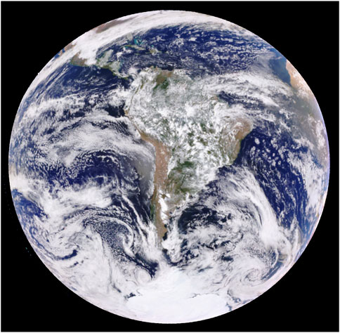
FIGURE 1. EPIC image acquired at 17:07 UTC on 1 January 2016 showing large cloud coverage in the Amazon region, an ideal region for studying near-cloud aerosol properties over land. EPIC image is publicly available on https://epic.gsfc.nasa.gov.

Section 2 describes the data sets used in the analysis. The analysis method is presented in Section 3. The results are presented in Section 4, followed by a summary and discussion of the results in the final section.

2 Data

We apply our 2LM to correct 3D radiative effects for Aqua MODIS in cloudy conditions. To reduce data volume, we use Aqua MODIS subset data from NASA’s A-Train data depot provided by NASA Goddard Earth Science Data and Information Service Center (GES DISC) (https://atrain.gesdisc.eosdis.nasa.gov/data/MAC/). Each data file is a subset of the original 5-min granule. Each subset MODIS image is 201 km wide with the CALIPSO ground track in the middle and 2030 km along-track, the same as the conventional 5-min granule (Savtchenko et al., 2008). Specifically, MAC04S1 for aerosol and MAC06S1 for cloud in the A-Train data depot are used. The CALIOP aerosol data are from NASA Langley Research Center’s Atmospheric Science Data Center (https://opendap.larc.nasa.gov/opendap/CALIPSO/). We focus on the Amazon region with the latitude range [20°S, 10°N] and longitude [20°W, 80°W] for the years 2016 and 2017.

2.1 MODIS data

The MODIS instrument on the Aqua satellite measures top-of-atmosphere (TOA) reflected solar and emitted terrestrial radiances at 36 wavelengths, ranging from 0.41 μm to 14 μm at moderate spatial resolution (nadir/subsatellite having 250 m for bands 1–2, 500 m for bands 3–7, 1 km for bands 8–36). The MODIS has a cross-track swath of 2330 km, providing the capability to view the entire globe every 1-2 days (Salomonson et al., 2006). There are three operational algorithms to provide daily aerosol retrievals. They are the Dark-Target (DT; Levy et al., 2013), Deep Blue (DB; Hsu et al., 2019), and Multiangle Implementation of Atmospheric Correction (MAIAC; Lyapustin et al., 2018), all developed at NASA Goddard Space Flight Center. In this study, we focus only on analyzing the performance of 2LM for correcting 3D radiative effects for DT aerosol retrievals. Note that DT is appropriate because the Amazon Forest is a large and uniform dark vegetated region (Kaufman et al., 1997a; Remer et al., 2005; Levy et al., 2013).

The MODIS DT algorithm consists of two entirely independent algorithms, one for retrieving aerosols over the ocean and the other over land. The development of the DT algorithm traced back to the launch of the Terra satellite (Kaufman et al., 1997a; Tanré et al., 1997; Remer et al., 2005; Levy et al., 2013). The algorithm uses dark surfaces as targets of opportunity to measure the contrast with the bright aerosol above and compares MODIS TOA reflectance observations over them with modeled reflectance properties (Lookup Tables) of scene-dependent aerosol optical models dominated by fine-sized particles (with radius << 1.0 µm) and coarse-sized particles (with radius >1.0 µm) to retrieve an appropriate solution. Whether over land or ocean, results of DT include spectral total aerosol optical depth (AOD), along with the relative contribution of fine-sized particles to the total AOD known as Fine Model Fraction or FMF.

The DT ocean algorithm is based on the fact that the spectral reflectance of the dark ocean surface is well known, and radiances at seven wavelengths (i.e., 0.47, 0.55, 0.66, 0.86, 1.24, 1.64, 2.11 μm) are used for aerosol retrievals. Aerosol properties are retrieved for 10 × 10 km² boxes using 20 × 20 pixels at 500-m resolution. In the retrieval processes, all 400 pixels must be identified as ocean pixels for the ocean algorithm to be applied. After screening pixels of clouds and marine sediments, the brightest 25% and darkest 25% of the remaining 500-m pixels are discarded. The remaining pixels are used for the retrieval. Sunglint pixels (assumed within 40° of specular reflection) are avoided in the retrieval. Using the average spectral reflectance as input, the algorithm retrieves aerosol properties, including aerosol spectral optical depth, Ångström Exponent (AE), and FMF. In addition, the algorithm reports the aggregated and averaged spectral reflectance used for the retrieval.

Over land and coastal areas, the DT land algorithm retrieves spectral AOD (0.47, 0.55, and 0.66 µm wavelengths) and FMF at 0.55 µm (Kaufman et al., 1997a; Remer et al., 2005; Levy et al., 2013). Pixels containing bright land, water, and snow/ice and cloudy pixels are masked out. Dark pixels are selected based on their reflectance at 2.11 µm, which must fall within the range of 0.01–0.25 to be selected. Pixels are then sorted according to their reflectance at 0.66 µm, and the darkest 20% and brightest 50% within each 10 km cell are discarded. Retrievals are performed on the remaining 30% of pixels. At launch, Kaufman et al. (1997b) suggested a simple parameterization to estimate surface reflectance at 0.47 μm (blue) and 0.66 μm (red) from TOA shortwave IR (SWIR) at 2.11 μm. Levy et al. (2007) found that the linear coefficients for surface reflectance at 2.11 μm and the reflectance at the blue and red band depend on NDVI characterized by TOA reflectance at 1.24 μm and 2.11 μm. Updated relationships of surface reflectance between the SWIR at 2.11 μm and visible (VIS) wavelength at 0.47 μm and 0.66 μm are used to estimate surface reflectance at the two VIS bands for aerosol retrievals (Levy et al., 2013). Note that a slightly modified DT algorithm has been used to retrieve aerosols at 3 km (Remer et al., 2013). We use only the 10 km aerosol product. Similar to the ocean algorithm, the land algorithm provides AOD, AE, and FMF and reports aggregated and averaged spectral reflectance used for retrieval.

In this study, we use average spectral reflectance selected for aerosol retrieval in MODIS data (MAC04S1 in A-Train data depot) for completely clear and liquid cloud-only scenes. The average spectral reflectance for clear and cloudy scenes with uncorrected and corrected situations is used as input to the Collection 6.1 (C6.1) offline code to retrieve aerosol optical depth.

Figure 2 shows an example of a full granule MODIS image in the Amazon region. Figure 3 presents images of a subset of MODIS data highlighted in Figure 2. It shows that the cloud field in the Amazon region has cloud optical depths ranging from near 0 to 150, cloud top pressure from near the surface (1,000 mb) to the tropopause (100 mb), and clouds in different thermodynamic phases (liquid and ice). The MODIS DT algorithm provides aerosol retrievals in such complicated cloud fields.

FIGURE 2

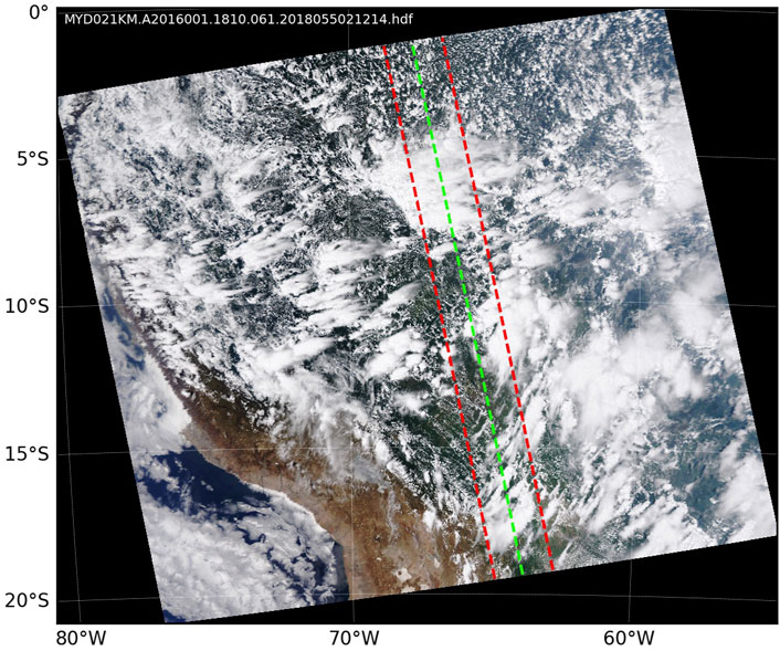
FIGURE 2. An example of Aqua MODIS image acquired at 18:10 UTC on 1 January 2016 with a subset of 201 km across the scan for A-Train data analysis indicated in dashed red and CALIPSO ground track in dashed green. For this case, the average solar zenith angle and solar azimuth angle are 28° and −120°, respectively, for MODIS and CALIPSO co-located observations.

FIGURE 3

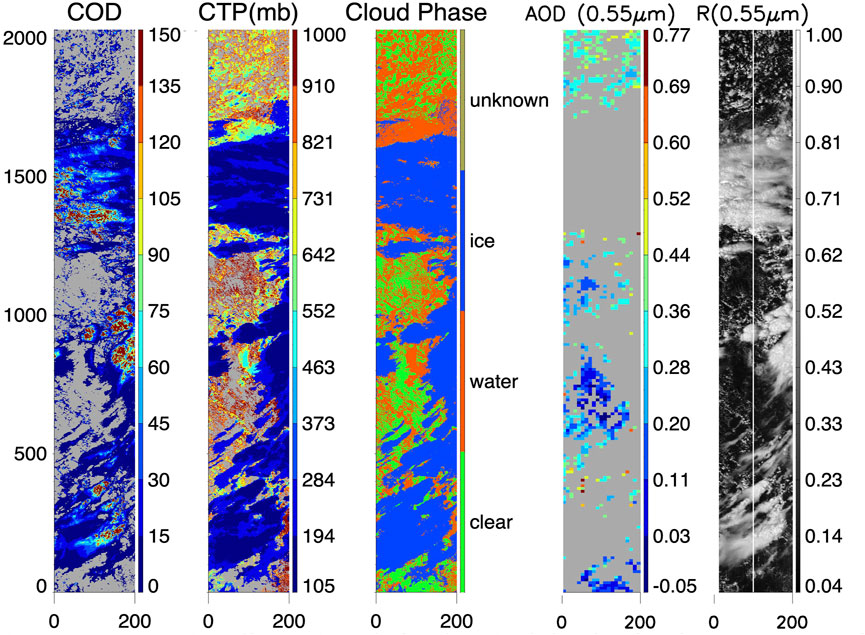
FIGURE 3. Example of MODIS operationally retrieved cloud optical depth (AOD), cloud top pressure (CTP), cloud phase, and aerosol optical depth (AOD) for the subset MODIS image (201 km across the scan and 2030 km along-track) in Figure 2. The reflectance at 0.55 μm is presented in the last column with a white line to indicate the CALIPSO ground track. The 1 km cloud data, 10 km aerosol data, and 1 km reflectance data are from MAC06S1, MAC04S1, and MAC021S1 obtained from the A-Train data depot, respectively.

We use 1 km resolution cloud properties from subset cloud products (MAC06S1 in the A-Train depot) for estimating cloud-induced reflectance enhancements due to cloud-molecular interactions and cloud-surface interactions (see Section 3.1 for details). The cloud properties include cloud optical depth, cloud top pressure, and cloud phase. Again, we consider liquid cloud-only scenes for cloudy conditions in a MODIS aerosol 10 × 10 km² box.

2.2 CALIOP data

The CALIOP uses three receiver channels: one measures the 1,064 nm backscatter intensity and two channels measure orthogonally polarized components of the 532 nm backscattered signal, from which the linear depolarization is derived. Flying at an altitude of 705 km above the Earth’s surface, the diameter of the laser footprint is 70 m, with successive footprints spaced by 333 m along the orbit track. The instrument has a fixed near-nadir view angle along-track in the forward direction (0.3° prior to November 2007 and 3° after that) to provide vertical profiles along the orbital path. The 532 nm backscatter signal is sampled every 30 m vertically from −0.5 km to 8.2 km. Between 8.2 km and 20.2 km altitude, profiles are averaged to 60 m in the vertical and every three successive shots are averaged together to give a horizontal resolution of 1 km (Winker et al., 2007; Hunt et al., 2009; Winker et al., 2009).

In CALIPSO aerosol retrievals, an assumed aerosol extinction-to-backscatter ratio (lidar ratio) is used to retrieve extinction for each layer from backscatter signals. The column aerosol optical depth is obtained by integrating the extinction from each layer. The values of the lidar ratio depend on the aerosol subtype. In the retrieval processes, for each aerosol layer detected, CALIPSO infers an aerosol subtype based on depolarization ratio at 532 nm, surface type, layer integrated attenuated backscatter, and aerosol layer height (Omar et al., 2009; Winker et al., 2009; Young and Vaughan, 2009; Kim et al., 2018).

We use CALIPSO Level 2 version 4 (V4) (Kim et al., 2018) 5 km aerosol layer product in this study. In a study to validate CALIPSO version 3 (V3), Schuster et al. (2012) compared CALIPSO-retrieved AOD with AERONET observations and found there is a negative bias in CALIPSO AOD. It is important to note that most of the discrepancy was caused by marine and dust aerosols (see Figure 7 in Schuster et al., 2012) and marine aerosols are problematic because CALIPSO is always offshore of the AERONET sites. CALIPSO V4 should have a smaller bias than V3 because the team increased the lidar ratio for marine and dust aerosols (Kim et al., 2018).

3 Methods of analysis

We apply the 2LM to correct MODIS reflectance for aerosol retrieval. The MODIS 10 km cells in the middle along-track in the subset data (Savtchenko et al., 2008) with aerosol retrieval are co-located with the 5 km CALIPSO grid (see Figure 2 in Kittaka et al., 2011) with the highest quality of aerosol retrieval (similar processes used by Schuster et al., 2012). The co-located MODIS AOD at 550 nm for clear and cloudy conditions (operational and corrected) and CALIPSO AOD at 532 nm are analyzed.

Note that the wavelength difference between MODIS (550 nm) and CALIPSO (532 nm) introduces discrepancies in AOD estimates from the two retrievals because AOD depends on wavelength. This difference is ∼3% for an Ångström exponent of 1 and ∼6% for an Ångström exponent of 2. This is considered relatively small compared to uncertainties in AOD of both CALIPSO (Winker et al., 2009) and MODIS (Remer et al., 2005), as explained by Kim et al. (2013). Therefore, this difference will be neglected in this study.

3.1 The two-layer model

We first briefly review the 2LM developed earlier for correcting clear-air reflectance enhancement due to cloud-molecular interactions (Marshak et al., 2008; Wen et al., 2016) and cloud-surface radiative interactions based on a stochastic Poisson model of the distribution of broken clouds (Titov, 1990; Kassianov, 2003; Zhuravleva and Marshak 2005; Wen et al., 2016).

For the cloud-induced reflectance enhancement, we consider two components for the two-layer system: the reflectance from a broken cloud field with a scattering molecular layer above it and the reflectance from the same broken cloud field but with the molecules in the upper layer causing only extinction, but not scattering to the viewing direction (Marshak et al., 2008; Wen et al., 2013). The two-layer system is schematically shown in Figure 4.

FIGURE 4

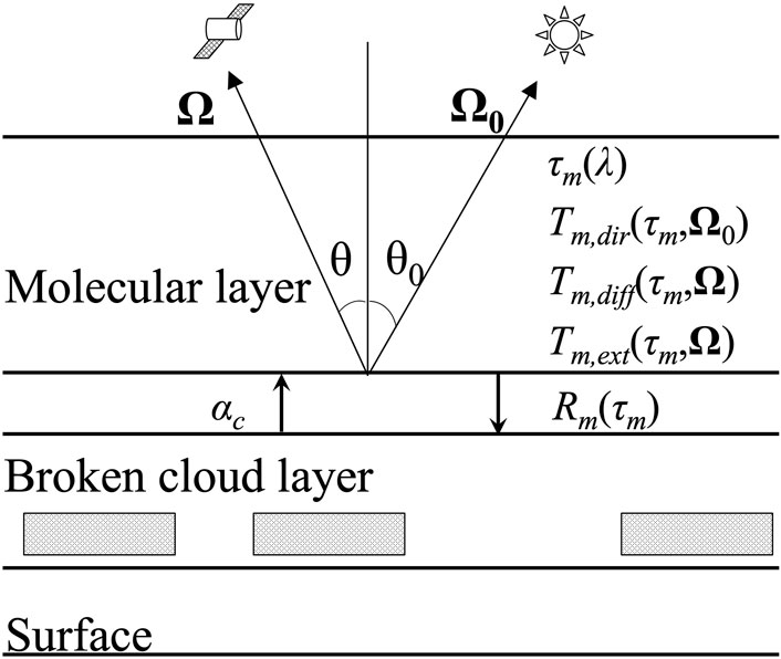
FIGURE 4. A schematic two-layer model of a broken cloud field (lower layer) and Rayleigh scatterers (upper layer) where $\lambda$ stands for wavelength; $\theta$ and ${\theta }_0$ are satellite viewing angle and solar zenith angle, respectively; $\mathrm{\Omega }$ and ${\mathrm{\Omega }}_{\mathbf{0}}$ are the directions of the satellite and the Sun, respectively; ${\tau }_m$ is the molecular optical depth of the upper layer; $T_{m,dir}$ is the transmittance of the molecular layer for the direct sunlight from above; $T_{m,diff}$ and $R_m$ are the transmittance and reflectance of the molecular layer for the diffuse radiation from the broken cloud layer, respectively; $T_{m,ext}$ is the extinction transmittance of the molecular layer for the diffuse radiation from the broken cloud layer in the direction of the satellite; and ${\alpha }_c$ is the albedo of the broken cloud field. Based on data from Figure 2 in Marshak et al. (2008).

The first reflectance ($r_1$) generated by the cloud reflected upward flux is simply the total TOA reflectance that includes molecular scattering, extinction, and multiple reflections between two layers. The second reflectance ($r_2$) generated by the same upward flux is the radiance with the molecular layer causing only extinction without scattering. The expressions for both reflectances are shown in Eqs1a, 1b:

$r_1\left(\lambda ,\mathbf{\Omega },{\mathbf{\Omega }}_{\mathbf{0}}\right)=\frac{{\alpha }_c{T}_{m,dir}\left({\tau }_m\left(\lambda \right),{\mathbf{\Omega }}_{\mathbf{0}}\right)T_{m,diff}\left({\tau }_m\left(\lambda \right),\mathbf{\Omega }\right)}{1-{\alpha }_c{R}_m\left({\tau }_m\left(\lambda \right)\right)}(\mathrm{1a})$

$r_2\left(\lambda ,\mathbf{\Omega },{\mathbf{\Omega }}_{\mathbf{0}}\right)=\frac{{\alpha }_c{T}_{m,dir}\left({\tau }_m\left(\lambda \right),{\mathbf{\Omega }}_{\mathbf{0}}\right)T_{m,ext}\left({\tau }_m\left(\lambda \right),\mathbf{\Omega }\right)}{1-{\alpha }_c{R}_m\left({\tau }_m\left(\lambda \right)\right)}(\mathrm{1b})$

where α_c is cloud albedo, τ_m(λ) is the molecular scattering optical depth above cloud top level for wavelength λ, Ω₀ and Ω are the directions to the Sun and the satellite, $T_{m,dir}$ and $T_{m,diff}$ are transmittances of the molecular layer for direct sunlight from above and diffuse radiation reflected from the cloud layer below, respectively, R_m is the reflectance of the molecular layer for upwelling radiation from the cloud layer, T_m,ext = exp(-τ_m(λ)/μ) is the transmittance of the molecular layer for upwelling radiation from the cloud layer due to extinction in the satellite viewing direction, where μ is the cosine of the satellite viewing zenith angle (VZA).

The reflectance difference (i.e., $r_1-r_2$) yields the molecule scattered reflectance in the two-layer system. The reflectance difference as a result of cloud reflection followed by molecular scattering is the cloud-induced reflectance enhancement (ΔR_m), as shown in Eq. 2

$∆R_m\left(\lambda ,\mathbf{\Omega },{\mathbf{\Omega }}_{\mathbf{0}}\right)=\frac{{\alpha }_c{T}_{m,dir}\left({\tau }_m\left(\lambda \right),{\mathbf{\Omega }}_{\mathbf{0}}\right)}{1-{\alpha }_c{R}_m\left({\tau }_m\left(\lambda \right)\right)}\left[T_{m,diff}\left({\tau }_m\left(\lambda \right),\mathbf{\Omega }\right)-T_{m,ext}\left({\tau }_m\left(\lambda \right),\mathbf{\Omega }\right)\right](2)$

Note that as the first-order approximation ignores the multiple reflections (or the denominator), the reflectance enhancement is proportional to cloud albedo α_c for a given cloud top height.

The input for the 2LM includes average cloud scene albedo, molecular optical depth above clouds, solar zenith angle (SZA), and satellite viewing geometry using 1 km cloud optical depth and cloud top pressure in level-2 cloud data (Platnick et al., 2003).

Sunlight scattered by broken clouds increases the downward diffuse radiative flux in nearby clear areas and subsequently leads to reflectance enhancement through surface reflection and atmospheric extinction. Thus, the reflectance enhancement ($∆R_s$) due to cloud-surface radiative interactions may be expressed as

$∆R_s\left(\lambda \right)=T_{clear}{\alpha }_s\left(\lambda \right)e^{-\frac{\tau \left(\lambda \right)}{\mu }}(3)$

where T_clear is the average cloud-induced clear area diffuse transmittance (i.e., the extra radiation that reaches the surface because of sideways scattering by clouds), ${\alpha }_s\left(\lambda \right)$ is the surface albedo, $\tau \left(\lambda \right)$ is the atmospheric optical depth, and μ is the cosine of VZA.

This study considers cumulus clouds over land. A stochastic Poisson model of the distribution of broken clouds (Titov, 1990; Kassianov, 2003; Zhuravleva and Marshak 2005) is applied to estimate downward diffuse radiative flux at the surface. The average cloud-induced clear area diffuse transmittance (T_clear) can be obtained from the Poisson model (Wen et al., 2016). The Poisson model is completely determined by cloud fractional cover, cloud geometric thickness, average horizontal size of clouds, and averaged cloud optical properties, including cloud optical depth, single scattering albedo, and scattering phase function. Those parameters are estimated from 1 km MODIS cloud data. MODIS AOD and Rayleigh scattering optical depth for atmospheric extinction are used to estimate atmospheric optical depth. Surface reflectance in MODIS aerosol product is used to estimate surface albedo.

The 3D corrected reflectance ($R_{3D}\left(\lambda \right)$) is defined as

$R_{3D}\left(\lambda \right)=R_{1D}\left(\lambda \right)-∆R_m\left(\lambda \right)-∆R_s\left(\lambda \right)(4)$

where $R_{1D}\left(\lambda \right)$ is the 1D spectral reflectance used for operational aerosol retrieval in the DT algorithm. The 3D corrected spectral reflectance ($R_{3D}\left(\lambda \right)$) is used as input to the DT algorithm to get 3D corrected aerosol properties.

The following is a summary of the 3D correction steps.

1. Identify MODIS 10 km boxes with aerosol retrievals that are partially covered by liquid clouds only by using 1 km cloud optical depth and cloud phase parameters. Here, we use COD for cloud mask. A pixel is defined as cloudy if COD is retrieved. Otherwise, it is clear. If a 10 km box contains cloudy pixels and all clouds are in the liquid phase, the aerosol box is considered for 3D correction.

2. For the identified 10 km boxes in step 1, we estimate the reflectance enhancement due to cloud-molecular interactions using Eq. 2. The averages of cloud albedo α_c, molecular layer reflectance ($R_m$), and transmittances ($T_{m,dir}$; $T_{m,diff}$; $T_{m,ext}$) in Eq. 2 are estimated using 1 km cloud optical depth data, cloud top pressure (for molecular optical thickness), and solar zenith angle and viewing angle provided in level-2 cloud product.

3. For the identified 10 km boxes in step 1, we estimate the reflectance enhancement due to cloud-surface interactions using Eq. 3. The average cloud-induced clear area diffuse transmittance ($T_{clear}$) is estimated using the Poisson model for estimating the reflectance enhancement due to cloud-surface interaction from Eq. 3. The input parameters to the Poisson model include cloud fraction, averages of cloud optical depth, cloud geometric thickness, and horizontal size of clouds in 10 km boxes. Those parameters, except cloud geometric thickness, are taken from 1 km level-2 cloud product. The statistics of cloud base height of 0.85 km in the Amazon region retrieved from Multi-angle Imaging SpectroRadiometer (MISR) (Böhm et al., 2019) and MODIS cloud top height are used to estimate cloud thickness. MODIS AOD and molecular optical depth of the atmosphere and viewing angle are used for accounting for the reflectance attenuation in Eq. 3. The estimates of cloud albedo, molecular transmittances in step 2, and the cloud-induced clear area diffuse transmittance in step 3 are calculated using pre-calculated look-up-tables (LUTs). Finally, the 3D corrected spectral reflectance is estimated from Eq. 4.

3.2 MODIS-CALIPSO Co-location and data screening

Both Aqua and CALIPSO fly in the A-train constellation in a 705 km sun-synchronous polar orbit with an equator-crossing time of approximately 1:30 PM local solar time. The orbit has a 16-day repeat cycle with cross-track errors of less than ±10 km (Stephens et al., 2002; Winker et al., 2007).

Since TOA reflectance is very strong over sunglint and aerosol properties are not retrieved from MODIS observations in sunglint regions, CALIPSO is located 215 km to the east of Aqua when crossing the equator on the day side of the orbit, such that the CALIPSO footprint remains outside of the sunglint pattern seen by the Aqua MODIS instrument. To minimize changes in cloud and aerosol properties between observations from the two satellites, the along-track separation is controlled to be less than 2 min with CALIPSO behind Aqua (Winker et al., 2007).

For each MODIS 10 km box with aerosol retrievals, we search CALIPSO daytime observations from orbit just behind Aqua; this is a similar process used by Kittaka et al. (2011). The criterion for a co-located pair of MODIS and CALIPSO AOD observations is that the distance between the centers of MODIS 10 km box and CALIPSO 5 km pixel is less than 10 km.

Since CALIPSO observations are used to test the 2LM, we consider only high-quality CALIPSO aerosol retrieval. Similar to the criteria in the study by Schuster et al. (2012), we require the CALIPSO Extinction QC flag for 532 nm to be equal to zero for all detected aerosol layers, indicating that a successful extinction solution was achieved with the default lidar ratio assigned to each layer. We also require the CALIPSO cloud and aerosol detection score (CAD Score) to be less than −20 for all detected layers.

As mentioned previously, we consider MODIS 10 km boxes with aerosol retrievals for clear scenes as a reference and cloudy scenes partially covered by low-level liquid clouds only. The clear scenes are determined by the COD provided in the level-2 cloud product. If there is no COD retrieval for all 1 km pixels in a 10 km box, the whole 10 km box is considered clear. We might have missed some optically thin or sub-pixel cloud that could be identified in the level-2 cloud mask. However, such clouds would likely have a small 3D radiative impact on reflectance enhancement and aerosol retrievals for nearby pixels.

4 Results

Before checking aerosol retrieval in cloud fields, we first examine the statistics (the mean, median, and standard deviation and the slope of the best fit) of MODIS and CALIPSO aerosol retrievals in clear conditions in the Amazon region. Figure 5 presents the scatterplot of MODIS AOD at 550 nm vs. CALIPSO AOD at 532 nm for clear conditions of 2-year data (2016 and 2017). There are over 10,000 pairs of co-located MODIS and CALIPOS retrievals. It is evident that the majority of AOD is smaller than 0.4 for both MODIS and CALIPSO. To focus on the most populated observations, we compare AOD from 0 to 1 for both MODIS and CALIPSO for both clear and cloudy conditions, like the analysis by Kittaka et al. (2011). The mean of MODIS AOD is 0.187, only 0.015 smaller than the mean of CALIPSO AOD of 0.201; the median of MODIS AOD is 0.149, which is very close to the median of CALIPSO AOD of 0.145; and the standard deviation of MODIS AOD is 0.155, which is slightly smaller than the standard deviation 0.173 of CALIPOS AOD. The best-fit line between MODIS and CALIPSO AOD has a slope of 0.87 and is relatively close to the one-to-one line in the scatterplot. In general, MODIS DT-retrieved AOD statistically agrees very well with CALIPSO AOD. We also noticed that the root-mean-square-error (RMSE) against CALIPSO measurement, as well as the RMSE of the best-fit line, are approximately the same (∼0.16). The relatively large RMSEs compared to the mean AOD are primarily due to large variability of both MODIS and CALIPSO AOD (σ ∼ 0.16). Note that the standard error of the mean $(\frac{\sigma }{\sqrt{n}})$ is very small compared to the retrieval uncertainties since the standard deviation (σ) of AOD is less than ∼0.25 and sample size (n) is quite large for both clear and cloudy conditions.

FIGURE 5

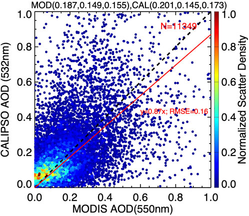
FIGURE 5. Comparison of MODIS AOD at 550 nm and co-located CALIPSO-retrieved AOD at 532 nm for clear conditions for MODIS 10 × 10 km² boxes in the Amazon region for the years 2016 and 2017. For these 2 years, 11,349 boxes are cloud-free. The mean, median, and standard deviation are indicated in parentheses at the top of the figure for both MODIS and CALIPSO. The best-fit line (y = 0.87x) between MODIS AOD and CALIPSO AOD is in red. The 1:1 line is plotted in dashed black for reference. The color represents the number of scattered points within a unit area in the X-Y plane normalized by the total number of scattered points.

Figure 6 shows the scatterplot of MODIS AOD from the operational DT algorithm and co-located CALIPSO AOD for areas partially covered by only liquid clouds in the Amazon region. There are more than 4,700 pairs of MODIS and CALIPSO AOD. It is evident that most of the scatter points between 0 and 0.4 are below the one-to-one line, showing that the MODIS-retrieved AOD is higher than the CALIPSO AOD. From clear to cloudy conditions, there is an increase in the mean and median of AOD for both MODIS and CALIPSO, suggesting a real change in AOD near clouds. However, the increase in the mean (0.075) and median (0.059) for MODIS is considerably larger than the increase in the mean (0.041) and median (0.02) for CALIPSO. The increase in the mean and median of MODIS AOD is likely to be largely due to cloud 3D radiative effects. The slope of the best-fit line is 0.78, which is significantly smaller than the slope for clear conditions in Figure 5. The standard deviation of MODIS AOD is slightly larger than that of CALIPSO.

FIGURE 6

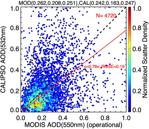
FIGURE 6. Comparison of MODIS AOD retrieved from the operational DT algorithm and CALIPSO-retrieved AOD for liquid cloud-only conditions for MODIS 10 × 10 km² boxes in the Amazon region for years 2016 and 2017. Aerosol was retrieved but the CF was not 0, and clouds were low liquid clouds. The mean, median, and standard deviation are indicated in parentheses at the top of the figure for both MODIS and CALIPSO. The best-fit line (y = 0.78x) between MODIS AOD and CALIPSO AOD is in red. The 1:1 line is plotted in dashed black for reference.

Figure 7 shows the scatterplot of the 3D corrected MODIS AOD and co-located CALIPSO AOD for the same pairs of observations as in Figure 6. The mean (0.230) and median (0.176) of corrected MODIS AOD are in better agreement with the mean (0.242) and median (0.163) of CALIPSO AOD than the uncorrected retrievals in Figure 6. The 3D correction also leads to improvement in the standard deviation of MODIS AOD and the slope of the best-fit line. The standard deviation of MODIS AOD is reduced from 0.251 for the operational retrieval to 0.239 for the corrected one. The slope of 0.83 after the 3D correction is significantly larger than the slope of 0.78 before the correction and much closer to the slope of 0.87 for the MODIS and CALIPSO AOD relationship for clear conditions. The improvement of the 3D correction can be seen by comparing CALIPSO retrievals, as shown in Table 1.

FIGURE 7

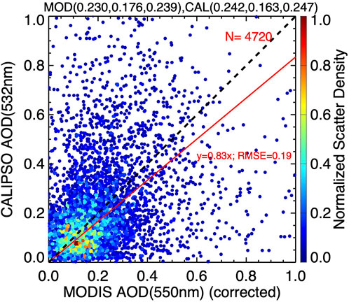
FIGURE 7. Similar to Figure 6, but for 3D corrected DT MODIS AOD vs. CALIPSO AOD. The mean, median, and standard deviation are indicated in the parenthesis at the top of the figure for both MODIS and CALIPSO. The best-fit line (y = 0.83x) between MODIS AOD and CALIPSO AOD is in red. The 1:1 line is plotted in dashed black for reference.

TABLE 1

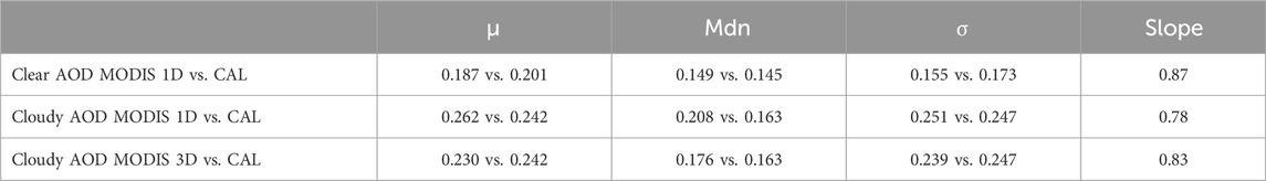
TABLE 1. Comparison of the statistics (mean (μ), median (Mdn), and standard deviation (σ)) of MODIS operationally retrieved AOD (MODIS 1D), 3D corrected AOD (MODIS 3D), and CALIPSO (CAL)-retrieved AOD for clear and cloudy conditions. The slopes of the best fit between MODIS and CALIPSO AOD are also presented.

Note that the RMSEs of the two linear fits are approximately the same, and the RMSE of MODIS AOD against CALIPSO AOD remains approximately the same (∼0.2) for both the operationally retrieved and the corrected MODIS AOD. This is mainly because the variability of both MODIS and CALIPSO AOD (σ ∼ 0.25) is much larger than the 3D correction for MODIS AOD (average ΔAOD ∼ 0.032).

Figure 8 compares the MODIS AOD retrieved from the operational DT algorithm and 3D effects corrected AOD presented in Figures 6, 7. It is evident that the majority of the scattered points are below the one-to-one line. There are some instances where the corrected AOD is slightly larger than the operationally retrieved AOD, with the largest difference (corrected – operational) less than 0.05 and the average difference (about 0.01) much smaller than the uncertainty of MODIS retrieval. On average, corrected AOD is 0.23 compared to 0.262 of the operationally retrieved AOD. The corrected AOD is on average approximately 14% lower than the operationally retrieved AOD.

FIGURE 8

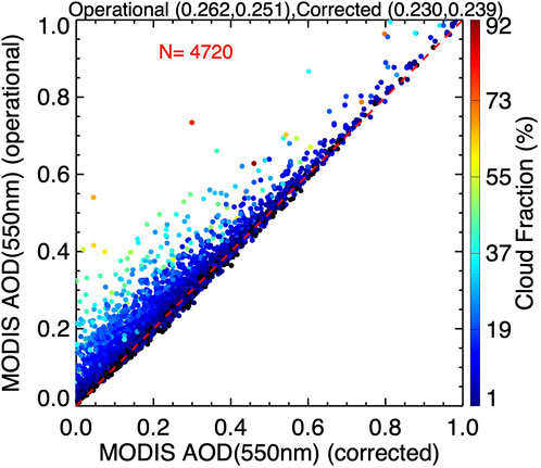
FIGURE 8. MODIS AOD retrieved from operational DT algorithm vs. corrected AOD at 550 nm. Generally, the corrected AOD is smaller than operationally retrieved AOD; however, there are some occasions when the corrected AOD is slightly larger than the operationally retrieved ones with the largest difference (corrected – operational) less than 0.05 and an average difference of approximately 0.01, much less than the uncertainty of MODIS retrieval (±0.05 ± 0.15τ). The mean and standard deviation are indicated in the parenthesis at the top of the figure for both operational and corrected MODIS AOD.

The magnitude of the 3D correction ($∆AOD=AOD\left(operational\right)-AOD\left(corrected\right)$) is evidently positively correlated with cloud fraction (CF), as indicated by the color scheme in Figure 8. This is because cloud albedo is positively correlated with CF and cloud-molecular interaction dominants in cloud 3D radiative interactions (Wen et al., 2008).

Figure 9 presents the statistics of the operationally retrieved and 3D corrected AOD, the 3D correction, and the sample distribution of MODIS retrievals as a function of CF. It is clear from Figure 9A that both operationally retrieved and 3D corrected AOD increase with CF, up to 0.6, and the rate of the increase for the corrected AOD is smaller compared to the operationally retrieved AOD; the positive correlation breaks down above CF of 0.6; the standard deviation increases with CF. As expected from Eq. 2, Figure 9B shows that the average 3D correction has a strong linear relation with CF in the range of CF up to 0.7. Note that there is a decrease in the average 3D correction from CF 0.6–0.7 to 0.7–0.8 bin. This is mainly because there are few MODIS AOD retrievals for nearly overcast situations (Figure 9C). The percentage correction ($∆AOD/AOD\left(corrected\right)\bullet 100$) increases with CF, starting from 7% for CF < 0.1, reaching a maximum of ∼50% near CF of 0.5 and decreases with CF. Figure 9C shows the frequency distribution of samples of MODIS aerosol retrieval as a function of cloud fraction. The number of samples of MODIS retrieval decreases nearly exponentially with cloud fraction. This is the nature of MODIS aerosol retrieval. As cloud fraction increases, there are fewer 10 km boxes that satisfy the selection criteria of the DT algorithm, resulting in fewer aerosol retrievals. This explains the breakdown of the positive correlation between MODIS AOD with CF near CF of 0.6, the increase of standard deviation with CF, and the non-smooth behavior of percentage correction for larger CF values.

FIGURE 9

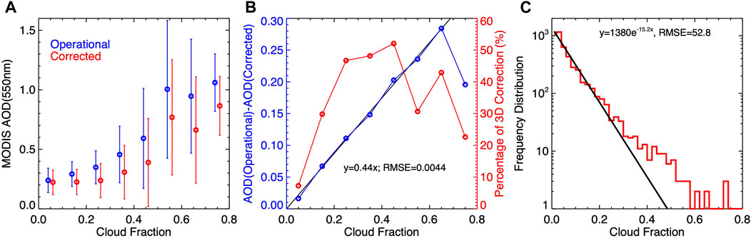
FIGURE 9. Statistics of the operationally retrieved and 3D corrected AOD, the 3D correction of AOD, and sample distribuition. (A) Dots are for average MODIS operationally retrieved (in blue) and 3D corrected (in red) AOD at 550 nm for different cloud fraction bins (i.e., 0–0.1, 0.1–0.2, 0.2–0.3, …). To avoid large values in the plot, the vertical bars show half of the standard deviations. The two AODs are plotted slightly off the center of the cloud fraction bin to show the difference. (B) Blue dots are for the average 3D correction of AOD in Panel (A) (left y-axis), and red dots are for the percentage of 3D correction (right y-axis) for different cloud fraction bins. Small RMSE in the best-fit line between the 3D correction and CF shows a strong linear relationship. (C) Frequency distribution of samples of MODIS aerosol retrieval as a function of cloud fraction. The number of samples of MODIS aerosol retrieval decreases nearly exponentially with cloud fraction.

It is interesting to note that even for a small amount of cloud cover (CF < 0.1), the average AOD for operational retrieval (∼0.24) and 3D corrected value (∼0.22) are significantly larger than the average AOD of 0.187 for completely clear conditions, suggesting different aerosol properties for all CF compared to clear conditions. Since the 3D correction is significant for small CF (e.g., ∼7% for CF < 0.1) (Figure 9B) and there are many more MODIS aerosol retrieval samples for small CF than large CF conditions (Figure 9C), it is important to correct 3D radiative effects for all CF conditions.

As the 3D radiation bias is one of six main hypotheses for satellite-derived cloud cover–AOD relationship (e.g., Quaas et al., 2010), we expect that the 3D corrected AOD will provide a more accurate cloud cover–AOD relationship for better understanding aerosol-cloud interactions.

In addition to AOD, aerosol size in cloud fields is an important parameter for better understanding aerosol-cloud interactions. In earlier studies, Várnai and Marshak (2015) analyzed regional MODIS aerosol data and showed an increase of Ångström Exponent (AE) with CF over the Atlantic Ocean. In a global analysis of MODIS aerosol products, they found that (1) in summertime, positive correlations dominate over much of the southern hemispheric oceans, but over northern hemispheric oceans, there are large areas with both positive and negative correlations; (2) in wintertime, the two hemispheres are much more similar to each other, with positive but weaker correlations over most oceans; and (3) there are large areas of both positive and negative correlations both over land and ocean (Várnai and Marshak, 2018). Yang et al. (2014) analyzed CALIPSO nighttime data from a large region over the Atlantic Ocean near the Azores. They found increases in the attenuated total color ratio (ratio of total backscatter at 1,064 nm over that at 532 nm) with CF, suggesting an increase in aerosol size (or the AE) with CF.

Here, we examine the impact of the 3D correction on the retrieval of aerosol size in cloud fields. Figure 10 presents aerosol AE and the fraction of AOD at 0.55 μm contributed by fine dominated model (or fine model fraction (FMF or η), see Remer et al., 2005; Levy et al., 2013). We focus on CF less than 0.5 because few retrieval samples are available for large CF. First, let’s examine the operational retrievals. It is evident that there is an increase in average AE and FMF with cloud fraction. As CF varies from 0.05 to 0.45, the average AE increases from ∼1.2 to ∼1.5, which is approximately a 25% increase in AE in the CF range concerned (Figure 10A). In the same CF range, the average FMF increases from ∼0.5 to ∼0.8, which is approximately a 60% increase in FMF in the CF range concerned (Figure 10B). The 3D correction leads to smaller values of both AE and FMF. The correction (uncorrected – corrected) in both AE and FMF increases with CF. As a result, the average 3D corrected AE and FMF do not show a significant dependence on CF.

FIGURE 10

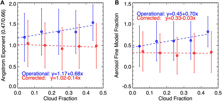
FIGURE 10. (A) Statistics of the operationally retrieved and 3D corrected aerosol AE. Dots are for the average MODIS operationally retrieved (in blue) and 3D corrected (in red) values for different cloud fraction bins (i.e., 0–0.1, 0.1–0.2, 0.2–0.3, 0.4–0.5) and the vertical bars are the standard deviation. (B) Is similar to (A) but for the fine model fraction (FMF). Because there are few MODIS aerosol retrieval samples available for CF > 0.5, we only show results for CF < 0.5.

5 Summary

There are difficulties in retrieving aerosol properties near clouds from passive remote sensing. Sunlight scattered by bright clouds into nearby clear regions can effectively enhance the clear area reflectance, consequently resulting in biases in aerosol retrievals. Without correcting for cloud 3D radiative effects, we may risk incorrect interpretation of satellite observations for aerosol–cloud interactions in a cloudy atmosphere.

In this study, we have used CALIPSO-retrieved AODs that are not affected by 3D cloud radiative effects to assess the 2LM for correcting MODIS retrievals for cloud 3D radiative contributions and to study aerosol properties in cloudy fields in the Amazon region. First, as a reference, we compared AOD from MODIS and CALIPSO for clear conditions. We found that the statistics of the co-located MODIS and CALIPSO AODs agree very well. Thus, CALISPO-retrieved AOD can be used to test our 3D correction algorithm for studying aerosol properties in cloud fields.

We found that there is an increase in average AOD from clear to cloudy conditions for both MODIS and CALIPSO. However, the increase is much larger for MODIS operationally retrieved AOD (∼0.075 or ∼40% in the mean and ∼0.059 or ∼40% in the median) compared to CALIPSO-retrieved AOD (∼0.021 or ∼20% in the mean and ∼0.018 or ∼12% in the median). After the correction for 3D radiative effects, the increase in MODIS AOD from clear to cloudy conditions reduced to ∼0.043 (∼23%) in the mean and ∼0.027 (∼18%) in the median, which is much closer to CALIPSO observations. On average, AOD in cloudy fields is approximately 20% larger than that in clear conditions.

Furthermore, we found that both operationally retrieved and 3D corrected AOD increase with CF for a large range of CF, and the rate of the increase for the corrected AOD is smaller compared to the operationally retrieved AOD; the 3D correction of MODIS AOD increases linearly with CF, approximately 7% for CF less than 0.1 and a maximum of ∼50% for CF of 0.5. We also found that MODIS AOD for cloudy scenes, even for cloud cover less than 0.1, is significantly larger than AOD in clear conditions, suggesting aerosols in cloudy conditions are characteristically different from those in clear conditions.

We also examined the impact of 3D correction on aerosol AE and FMF. We found that the operationally retrieved average AE and FMF depend strongly on CF, with an increase of ∼25% in AE and an increase of ∼60% in FMF as CF increases from 0.05 to 0.45. The 3D correction leads to smaller values of both AE and FMF and the corrections increase with CF. The averages of 3D corrected AE and FMF are almost independent of CF. Thus, the 3D corrected AOD will provide more accurate cloud cover–AOD relationship and aerosol size information for better understanding aerosol–cloud interactions.

Data availability statement

The datasets presented in this study can be found in online repositories. The names of the repository/repositories and accession number(s) can be found below: https://atrain.gesdisc.eosdis.nasa.gov/data/MAC/, https://opendap.larc.nasa.gov/opendap/CALIPSO/ (last access: 9 January 2024).

Author contributions

GW: Conceptualization, Formal Analysis, Investigation, Methodology, Writing–original draft, Writing–review and editing. AM: Conceptualization, Formal Analysis, Investigation, Methodology, Writing–original draft, Project administration. RL: Software, Writing–review and editing. GS: Methodology, Writing–review and editing.

Funding

The author(s) declare that financial support was received for the research, authorship, and/or publication of this article. This work was supported by NASA CloudSat/CALIPSO program under proposal solicitation number NNH21ZDA001N-CCST.

Acknowledgments

We gratefully acknowledge the support for this research from the NASA Radiation Sciences Program managed by Dr. Hal Maring and the CALIPSO Program managed by Dr. David Considine. The Aqua MODIS subset data, as part of the A-Train data set, were obtained from NASA Goddard Earth Science Data and Information Service Center (GES DISC). The CALIPSO data were obtained from the NASA Langley Research Center Atmospheric Science Data Center (ASDC).

Conflict of interest

The authors declare that the research was conducted in the absence of any commercial or financial relationships that could be construed as a potential conflict of interest.

Publisher’s note

All claims expressed in this article are solely those of the authors and do not necessarily represent those of their affiliated organizations, or those of the publisher, the editors and the reviewers. Any product that may be evaluated in this article, or claim that may be made by its manufacturer, is not guaranteed or endorsed by the publisher.

References

Bar-Or, R. Z., Koren, I., Altaratz, O., and Fredj, E. (2012). Radiative properties of humidified aerosols in cloudy environment. Atmos. Res. 118, 280–294. doi:10.1016/j.atmosres.2012.07.014

CrossRef Full Text | Google Scholar

Böhm, C., Sourdeval, O., Mülmenstädt, J., Quaas, J., and Crewell, S. (2019). Cloud base height retrieval from multi-angle satellite data. Atmos. Meas. Tech. 12 (3), 1841–1860. doi:10.5194/amt-12-1841-2019

CrossRef Full Text | Google Scholar

Charlson, R. J., Ackerman, A. S., Bender, F. A.-M., Anderson, T. L., and Liu, Z. (2007). On the climate forcing consequences of the albedo continuum between cloudy and clear air. Tellus 59, 715–727. doi:10.1111/j.1600-0889.2007.00297.x

CrossRef Full Text | Google Scholar

Hsu, N. C., Lee, J., Sayer, A. M., Kim, W., Bettenhausen, C., and Tsay, S. C. (2019). VIIRS deep blue aerosol products over land: extending the EOS long-term aerosol data records. J. Geophys. Res. Atmos. 124, 4026–4053. doi:10.1029/2018JD029688

CrossRef Full Text | Google Scholar

Hunt, W. H., Winker, D. M., Vaughan, M. A., Powell, K. A., Lucker, P. L., and Weimer, C. (2009). CALIPSO lidar description and performance assessment. J. Atmos. Ocean. Tech. 26, 1214–1228. doi:10.1175/2009jtecha1223.1

CrossRef Full Text | Google Scholar

IPCC (2013). in Climate change 2013: the physical science basis. Contribution of working group I to the fifth assessment report of the intergovernmental panel on climate change. Editors T. F. Stocker, D. Qin, G.-K. Plattner, M. Tignor, S. K. Allen, J. Boschunget al. (Cambridge, United Kingdom and New York, NY, USA: Cambridge University Press), 1535.

Google Scholar

Jeong, M. J., and Li, Z. (2010). Separating real and apparent effects of cloud, humidity, and dynamics on aerosol optical thickness near cloud edges. J. Geophys. Res. 115, D00K32. doi:10.1029/2009JD013547

CrossRef Full Text | Google Scholar

Kassianov, E. (2003). Stochastic radiative transfer in multilayer broken clouds. Part I: markovian approach. J. Quant. Spectrosc. Radiat. Transf. 77, 373–393. doi:10.1016/S0022-4073(02)00170-X

CrossRef Full Text | Google Scholar

Kassianov, E. I., and Ovtchinnikov, M. (2008). On reflectance ratios and aerosol optical depth retrieval in the presence of cumulus clouds. Geophys. Res. Lett. 35, L06807. doi:10.1029/2008GL033231

CrossRef Full Text | Google Scholar

Kaufman, Y. J., Tanré, D., Remer, L., Chu, A., Vermote, E., Chu, A., et al. (1997a). Operational remote sensing of tropospheric aerosol over land from EOS Moderate Resolution Imaging Spectroradiometer. J. Geophys. Res. 102, 17051–17067. doi:10.1029/96jd03988

CrossRef Full Text | Google Scholar

Kaufman, Y. J., Wald, A., Remer, L. A., Gao, B. C., Li, R. R., and Flynn, L. (1997b). The MODIS 2.1-μm channel-correlation with visible reflectance for use in remote sensing of aerosol. IEEE Trans. Geosci. Remote Sens. 35, 1286–1298. doi:10.1109/36.628795

CrossRef Full Text | Google Scholar

Kim, M.-H., Kim, S.-W., Yoon, S.-C., and Omar, A. H. (2013). Comparison of aerosol optical depth between CALIOP and MODIS-Aqua for CALIOP aerosol subtypes over the ocean. J. Geophys. Res. Atmos. 118 (23), 13–241. doi:10.1002/2013jd019527

CrossRef Full Text | Google Scholar

Kim, M.-H., Omar, A., Tackett, J., Vaughan, M., Winker, D., Trepte, C., et al. (2018). The CALIPSO version 4 automated aerosol classification and lidar ratio selection algorithm. Atmos. Meas. Tech. 11, 6107–6135. doi:10.5194/amt-11-6107-2018

PubMed Abstract | CrossRef Full Text | Google Scholar

King, M. D., Kaufman, Y. J., Menzel, W. P., and Tanré, D. (1992). Remote sensing of cloud, aerosol, and water vapor properties from the moderate resolution imaging spectrometer (MODIS). IEEE Trans. geoscience remote Sens. 30 (1), 2–27. doi:10.1109/36.124212

CrossRef Full Text | Google Scholar

King, M. D., Platnick, S. E., Menzel, W. P., Ackerman, S. A., and Hubandks, P. A. (2013). Spatial and temporal distribution of clouds observed by MODIS onboard the Terra and Aqua satellites. IEEE Trans. Geoscience Remote Sens. 51, 3826–3852. doi:10.1109/TGRS.2012.2227333

CrossRef Full Text | Google Scholar

Kittaka, C., Winker, D. M., Vaughan, M. A., Omar, A., and Remer, L. A. (2011). Intercomparison of column aerosol optical depths from CALIPSO and MODIS-Aqua. Atmos. Meas. Tech. 4, 131–141. doi:10.5194/amt-4-131-2011

CrossRef Full Text | Google Scholar

Koren, I., Remer, L. A., Kaufman, Y. J., Rudich, Y., and Martins, J. V. (2007). On the twilight zone between clouds and aerosols. Geophys. Res. Lett. 34, L08805. doi:10.1029/2007GL029253

CrossRef Full Text | Google Scholar

Levy, R. C., Mattoo, S., Mattoo, S., Vermote, E. F., and Kaufman, Y. J. (2007). Second-generation operational algorithm: retrieval of aerosol properties over land from inversion of moderate resolution imaging spectroradiometer spectral reflectance. J. Geophys. Res. Atmos. 112 (D13). doi:10.1029/2006JD007815

CrossRef Full Text | Google Scholar

Levy, R. C., Mattoo, S., Munchak, L. A., Remer, L. A., Sayer, A. M., Patadia, F., et al. (2013). The Collection 6 MODIS aerosol products over land and ocean. Atmos. Meas. Tech. 6 (11), 2989–3034. doi:10.5194/amt-6-2989-2013

CrossRef Full Text | Google Scholar

Loeb, N. G., and Schuster, G. L. (2008). An observational study of the relationship between cloud, aerosol and meteorology in broken low-level cloud conditions. J. Geophys. Res. 113, D14214. doi:10.1029/2007JD009763

CrossRef Full Text | Google Scholar

Lyapustin, A., Wang, Y., Korkin, S., and Huang, D. (2018). MODIS Collection 6 MAIAC algorithm. Atmos. Meas. Tech. 11 (10), 5741–5765. doi:10.5194/amt-11-5741-2018

CrossRef Full Text | Google Scholar

Marshak, A., Wen, G., Coakley, J., Remer, L., Loeb, N. G., and Cahalan, R. F. (2008). A simple model for the cloud adjacency effect and the apparent bluing of aerosols near clouds. J. Geophys. Res. 113 (D14), S17. doi:10.1029/2007JD009196

CrossRef Full Text | Google Scholar

Martins, V. S., Novo, E. M., Lyapustin, A., Aragão, L. E., Freitas, S. R., and Barbosa, C. C. (2018). Seasonal and interannual assessment of cloud cover and atmospheric constituents across the Amazon (2000–2015): insights for remote sensing and climate analysis. ISPRS J. Photogrammetry Remote Sens. 145, 309–327. doi:10.1016/j.isprsjprs.2018.05.013

CrossRef Full Text | Google Scholar

Omar, A., Winker, D., Kittaka, C., Vaughan, M., Liu, Z., Hu, Y., et al. (2009). The CALIPSO automated aerosol classification and lidar ratio selection algorithm. J. Atmos. Ocean. Tech. 26, 1994–2014. doi:10.1175/2009jtecha1231.1

CrossRef Full Text | Google Scholar

Parkinson, C. L. (2022). The earth-observing Aqua satellite mission: 20 Years and counting. Earth Space Sci. 9 (9), e2022EA002481. doi:10.1029/2022ea002481

PubMed Abstract | CrossRef Full Text | Google Scholar

Platnick, S., King, M. D., Ackerman, S. A., Menzel, W. P., Baum, B. A., Riédi, J. C., et al. (2003). The MODIS cloud products: algorithms and examples from Terra. IEEE Trans. geoscience Remote Sens. 41 (2), 459–473. doi:10.1109/tgrs.2002.808301

CrossRef Full Text | Google Scholar

Quaas, J., Stevens, B., Stier, P., and Lohmann, U. (2010). Interpreting the cloud cover–aerosol optical depth relationship found in satellite data using a general circulation model. Atmos. Chem. Phys. 10 (13), 6129–6135. doi:10.5194/acp-10-6129-2010

CrossRef Full Text | Google Scholar

Redemann, J., Zhang, Q., Russell, P. B., Livingston, J. M., and Remer, L. A. (2009). Case studies of aerosol remote sensing in the vicinity of clouds. J. Geophys. Res. Atmos. 114 (6). doi:10.1029/2008JD010774

CrossRef Full Text | Google Scholar

Remer, L. A., Kaufman, Y. J., Tanré, D., Mattoo, S., Chu, D. A., Martins, J. V., et al. (2005). The MODIS aerosol algorithm, products, and validation. J. Atmos. Sci. 62 (4), 947–973. doi:10.1175/jas3385.1

CrossRef Full Text | Google Scholar

Remer, L. A., Levy, R. C., Mattoo, S., Tanré, D., Gupta, P., Shi, Y., et al. (2020). The dark target algorithm for observing the global aerosol system: past, present, and future. Remote Sens. 12 (18), 2900. doi:10.3390/rs12182900

CrossRef Full Text | Google Scholar

Remer, L. A., Mattoo, S., Levy, R. C., and Munchak, L. A. (2013). MODIS 3 km aerosol product: algorithm and global perspective. Atmos. Meas. Tech. 6 (7), 1829–1844. doi:10.5194/amt-6-1829-2013

CrossRef Full Text | Google Scholar

Salomonson, V. V., Barnes, W., and Masuoka, E. J. (2006). Introduction to MODIS and an overview of associated activities. Earth Science Satellite Remote Sensing: Vol. 1: Science and Instruments, 12–32. doi:10.1007/978-3-540-37293-6_2

CrossRef Full Text | Google Scholar

Savtchenko, A., Kummerer, R., Smith, P., Gopalan, A., Kempler, S., and Leptoukh, G. (2008). A-train data depot: Bringing atmospheric measurements together. IEEE transactions on geoscience and remote sensing 46 (10), 2788–2795. doi:10.1109/TGRS.2008.917600

CrossRef Full Text | Google Scholar

Schuster, G. L., Vaughan, M., MacDonnell, D., Su, W., Winker, D., Dubovik, O., et al. (2012). Comparison of CALIPSO aerosol optical depth retrievals to AERONET measurements, and a climatology for the lidar ratio of dust. Atmos. Chem. Phys. 12 (16), 7431–7452. doi:10.5194/acp-12-7431-2012

CrossRef Full Text | Google Scholar

Spencer, R. S., Levy, R. C., Remer, L. A., Mattoo, S., Arnold, G. T., Hlavka, D. L., et al. (2019). Exploring aerosols near clouds with high-spatial-resolution aircraft remote sensing during SEAC4RS. J. Geophys. Res. Atmos. 124 (4), 2148–2173. doi:10.1029/2018jd028989

PubMed Abstract | CrossRef Full Text | Google Scholar

Stephens, G. L., Vane, D. G., Boain, R. J., Mace, G. G., Sassen, K., Wang, Z., et al. (2002). The CloudSat mission and the A-Train: a new dimension of space-based observations of clouds and precipitation. Bull. Am. Meteorological Soc. 83 (12), 1771–1790. doi:10.1175/bams-83-12-1771

CrossRef Full Text | Google Scholar

Su, W., Schuster, G. L., Loeb, N. G., Rogers, R. R., Ferrare, R. A., Hostetler, C. A., et al. (2008). Aerosol and cloud interaction observed from high spectral resolution lidar data. J. Geophys. Res. Atmos. 113 (24). doi:10.1029/2008JD010588

CrossRef Full Text | Google Scholar

Tackett, J. L., and Di Girolamo, L. (2009). Enhanced aerosol backscatter adjacent to tropical trade wind clouds revealed by satellite-based lidar. Geophys. Res. Lett. 36 (14). doi:10.1029/2009GL039264

CrossRef Full Text | Google Scholar

Tanré, D., Kaufman, Y. J., Herman, M., and Mattoo, S. (1997). Remote sensing of aerosol properties over oceans using the MODIS/EOS spectral radiances. J. Geophys. Res. Atmos. 102 (14), 16971–16988. doi:10.1029/96jd03437

CrossRef Full Text | Google Scholar

Titov, G. A. (1990). Statistical description of radiation transfer in clouds. J. Atmos. Sci. 47 (1), 24–38. doi:10.1175/1520-0469(1990)047<0024:SDORTI>2.0.CO;2

CrossRef Full Text | Google Scholar

Twohy, C. H., Coakley, J. A., and Tahnk, W. R. (2009). Effect of changes in relative humidity on aerosol scattering near clouds. J. Geophys. Res. Atmos. 114 (5). doi:10.1029/2008JD010991

CrossRef Full Text | Google Scholar

Várnai, T., and Marshak, A. (2011). Global CALIPSO observations of aerosol changes near clouds. IEEE Geoscience Remote Sens. Lett. 8 (1), 19–23. doi:10.1109/LGRS.2010.2049982

CrossRef Full Text | Google Scholar

Várnai, T., and Marshak, A. (2012). Analysis of co-located MODIS and CALIPSO observations near clouds. Atmos. Meas. Tech. 5 (2), 389–396. doi:10.5194/amt-5-389-2012

CrossRef Full Text | Google Scholar

Várnai, T., and Marshak, A. (2015). Effect of cloud fraction on near-cloud aerosol behavior in the MODIS atmospheric correction ocean color product. Remote Sens. 7 (5), 5283–5299. doi:10.3390/rs70505283

CrossRef Full Text | Google Scholar

Várnai, T., and Marshak, A. (2018). Satellite observations of cloud-related variations in aerosol properties. Atmosphere 9 (11), 430. doi:10.3390/atmos9110430

CrossRef Full Text | Google Scholar

Várnai, T., Marshak, A., and Eck, T. F. (2017). Observation-based study on aerosol optical depth and particle size in partly cloudy regions. J. Geophys. Res. Atmos. 122 (18), 10013–10024. doi:10.1002/2017jd027028

PubMed Abstract | CrossRef Full Text | Google Scholar

Wen, G., Marshak, A., and Cahalan, R. F. (2008). Importance of molecular Rayleigh scattering in the enhancement of clear sky reflectance in the vicinity of boundary layer cumulus clouds. J. Geophys. Res. Atmos. 113 (24). doi:10.1029/2008JD010592

CrossRef Full Text | Google Scholar

Wen, G., Marshak, A., Levy, R. C., Remer, L. A., Loeb, N. G., Várnai, T., et al. (2013). Improvement of MODIS aerosol retrievals near clouds. J. Geophys. Res. Atmos. 118 (16), 9168–9181. doi:10.1002/jgrd.50617

CrossRef Full Text | Google Scholar

Wen, G., Marshak, A., Várnai, T., and Levy, R. (2016). Testing the two-layer model for correcting near-cloud reflectance enhancement using LES/SHDOM-simulated radiances. J. Geophys. Res. Atmos. 121 (16), 9661–9674. doi:10.1002/2016JD025021

PubMed Abstract | CrossRef Full Text | Google Scholar

Winker, D. M., Hunt, W. H., and McGill, M. J. (2007). Initial performance assessment of CALIOP. Geophys. Res. Lett. 34 (19). doi:10.1029/2007gl030135

CrossRef Full Text | Google Scholar

Winker, D. M., Pelon, J., Coakley, J. A., Ackerman, S. A., Charlson, R. J., Colarco, P., et al. (2010). The CALIPSO mission: a global 3D view of aerosols and clouds. B. Am. Meteorol. Soc. 91, 1211–1229. doi:10.1175/2010BAMS3009.1

CrossRef Full Text | Google Scholar

Winker, D. M., Vaughan, M. A., Omar, A., Hu, Y., Powell, K. A., Liu, Z., et al. (2009). Overview of the CALIPSO mission and CALIOP data processing algorithms. J. Atmos. Ocean. Technol. 26 (11), 2310–2323. doi:10.1175/2009jtecha1281.1

CrossRef Full Text | Google Scholar

Yang, W., Marshak, A., Várnai, T., and Wood, R. (2014). CALIPSO observations of near-cloud aerosol properties as a function of cloud fraction. Geophys. Res. Lett. 41 (24), 9150–9157. doi:10.1002/2014gl061896

CrossRef Full Text | Google Scholar

Young, S. A., and Vaughan, M. A. (2009). The retrieval of profiles of particulate extinction from cloud-aerosol lidar infrared pathfinder satellite observations (CALIPSO) data: algorithm description. J. Atmos. Ocean. Technol. 26 (6), 1105–1119. doi:10.1175/2008jtecha1221.1

CrossRef Full Text | Google Scholar

Zhang, J., Reid, J. S., and Holben, B. N. (2005). An analysis of potential cloud artifacts in MODIS over ocean aerosol optical thickness products. Geophys. Res. Lett. 32 (15). doi:10.1029/2005GL023254

CrossRef Full Text | Google Scholar

Zhuravleva, T. B., and Marshak, A. L. (2005). On the validation of the Poisson model of broken clouds. Izvestiya Atmos. Ocean. Phys. 41 (6), 713–725.

Google Scholar